Transfer Function with Nonlinear Characteristics Definition Based on Multidimensional Laplace Transform and its Application to Forced Response Power Systems †

Abstract
:1. Introduction
2. Modal Series Forced Response
2.1. Linearization Process
2.2. Time Response under Impulse Function Input
2.3. Synthetic Example
3. Concept of Transfer Function with Nonlinear Characteristics
3.1. Introduction
- ➢
- The order of any transfer function is as high as the number of state variables included in the model; i.e., in large power systems there are many thousands of states; most of those poles or eigenvalues are not observable from any signal in the system.
- ➢
- An input signal applied to a power system will usually excite many modes, which will be reflected in different output signals and locations in the system.
- ➢
- Despite a transfer function is usually defined as a ratio of polynomials, it can be expressed as a sum of residues over a first order pole.
- ➢
- Transfer function analysis assumes that initial conditions are out of concern and the output is only a function of the forced function.
3.2. Theoretical Basis of Nonlinear Characteristic in Transfer Function
- They characterize a nonlinear system uniquely. Each nonlinear system has a unique transfer function, no matter what state space realization one starts with.
- They provide an input–output description of the nonlinear system.
- They allow the use of transfer function algebra, to combine systems in series, parallel or feedback connection.
- The first part is called forced response, which consists of the steady state part.
- The second one, called natural response, consists of the transient part, formed by a sum of exponentials, whose values depend on the applied disturbance.
3.3. Volterra Functional Expansion
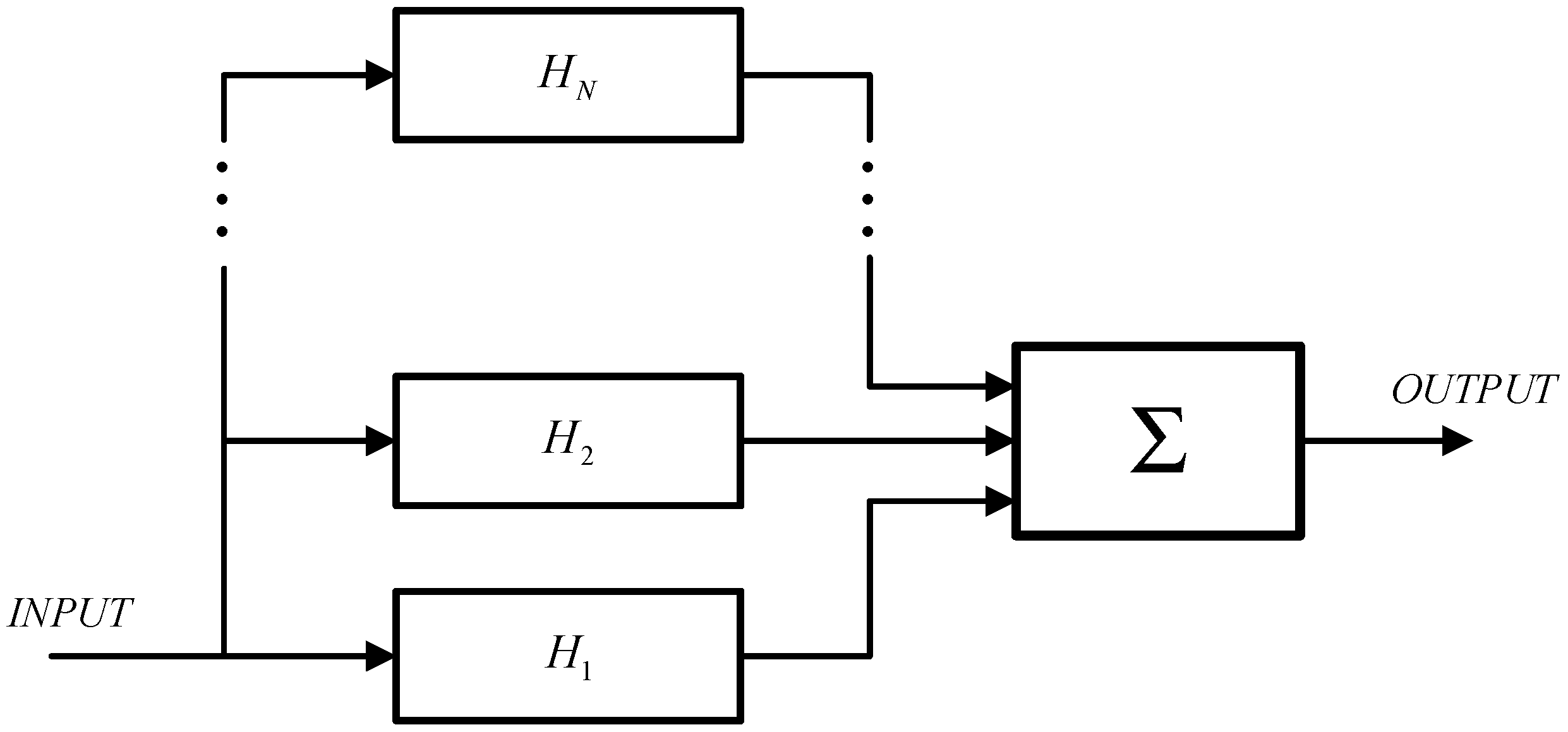
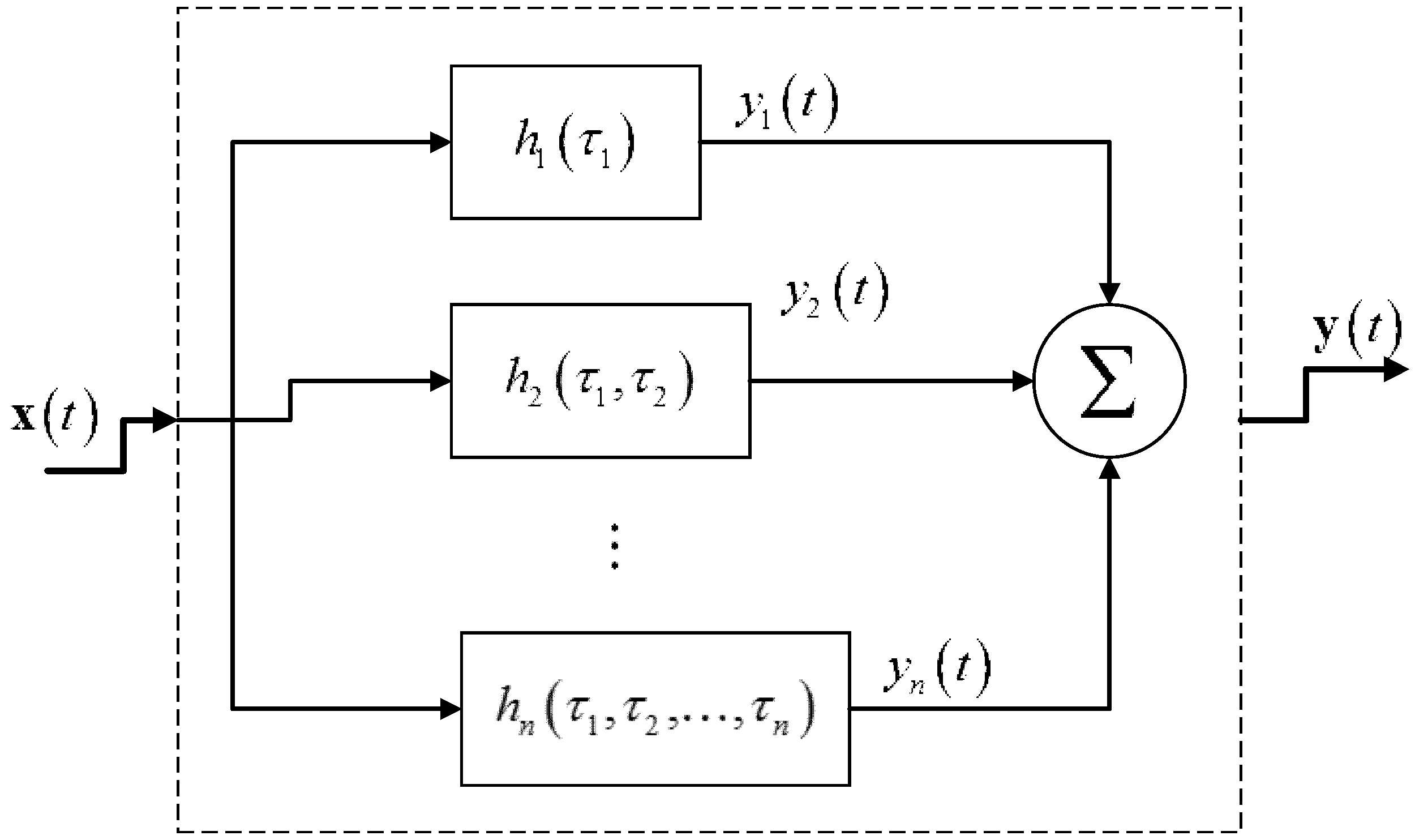
- The generalized functional representation shows a nonlinear system as a parallel bank of systems that are nth order nonlinear systems.
- They have an impulse-response function associated with them.
3.4. Analytical Deduction
4. Application to a Power System Model
4.1. Classical Model
- First order terms
- Second order termswhich is associated to,
- Third order termsor,
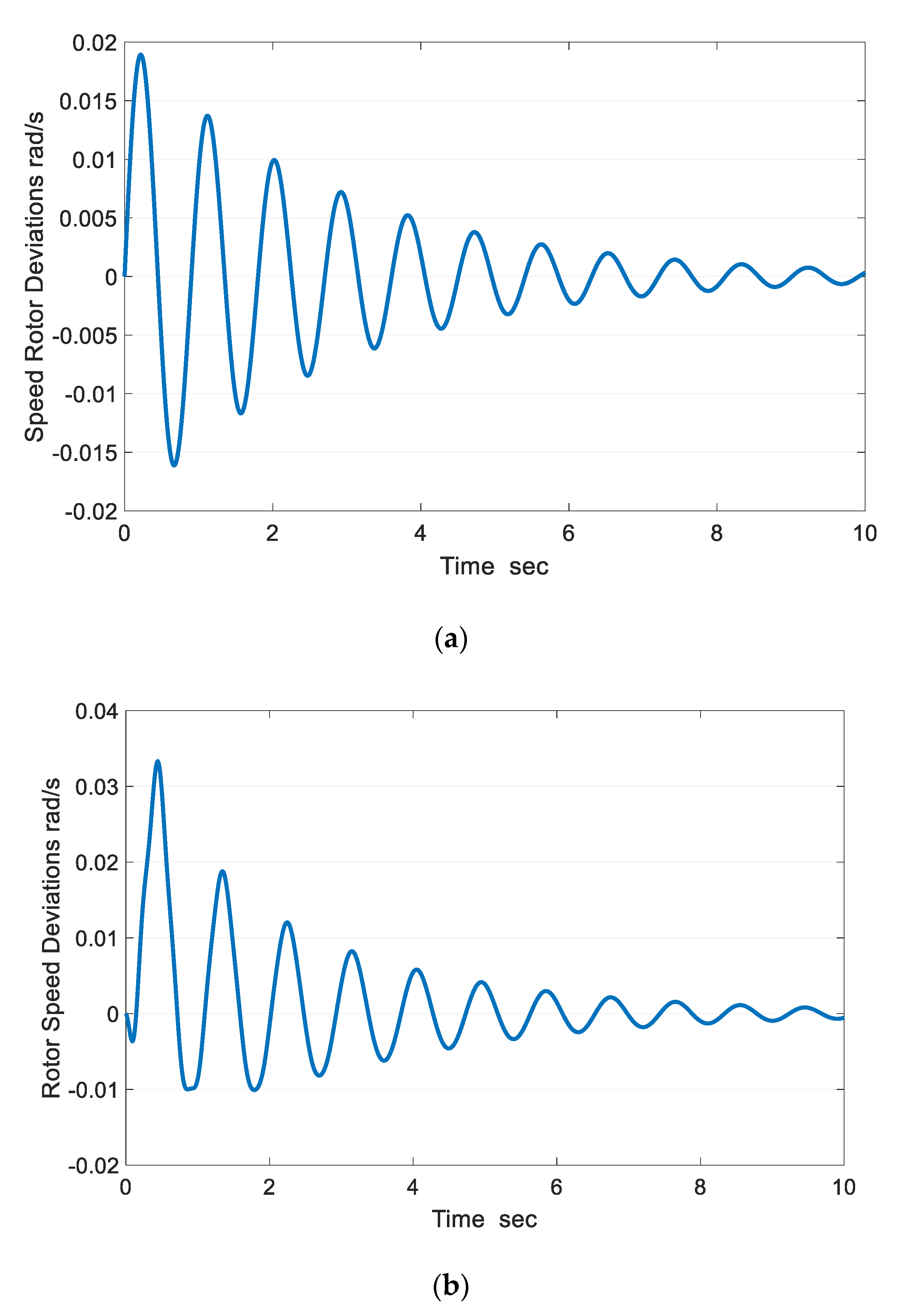
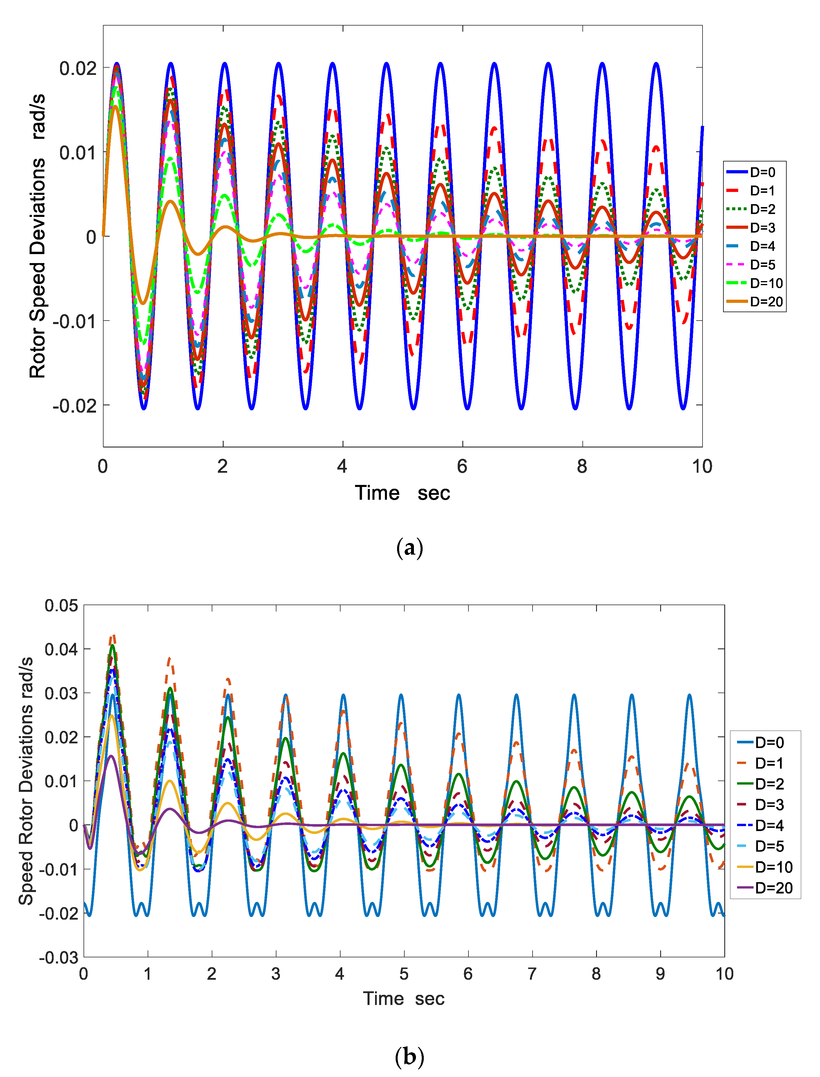
4.2. Step Input Response
5. Application to a Multimachine Power System Model
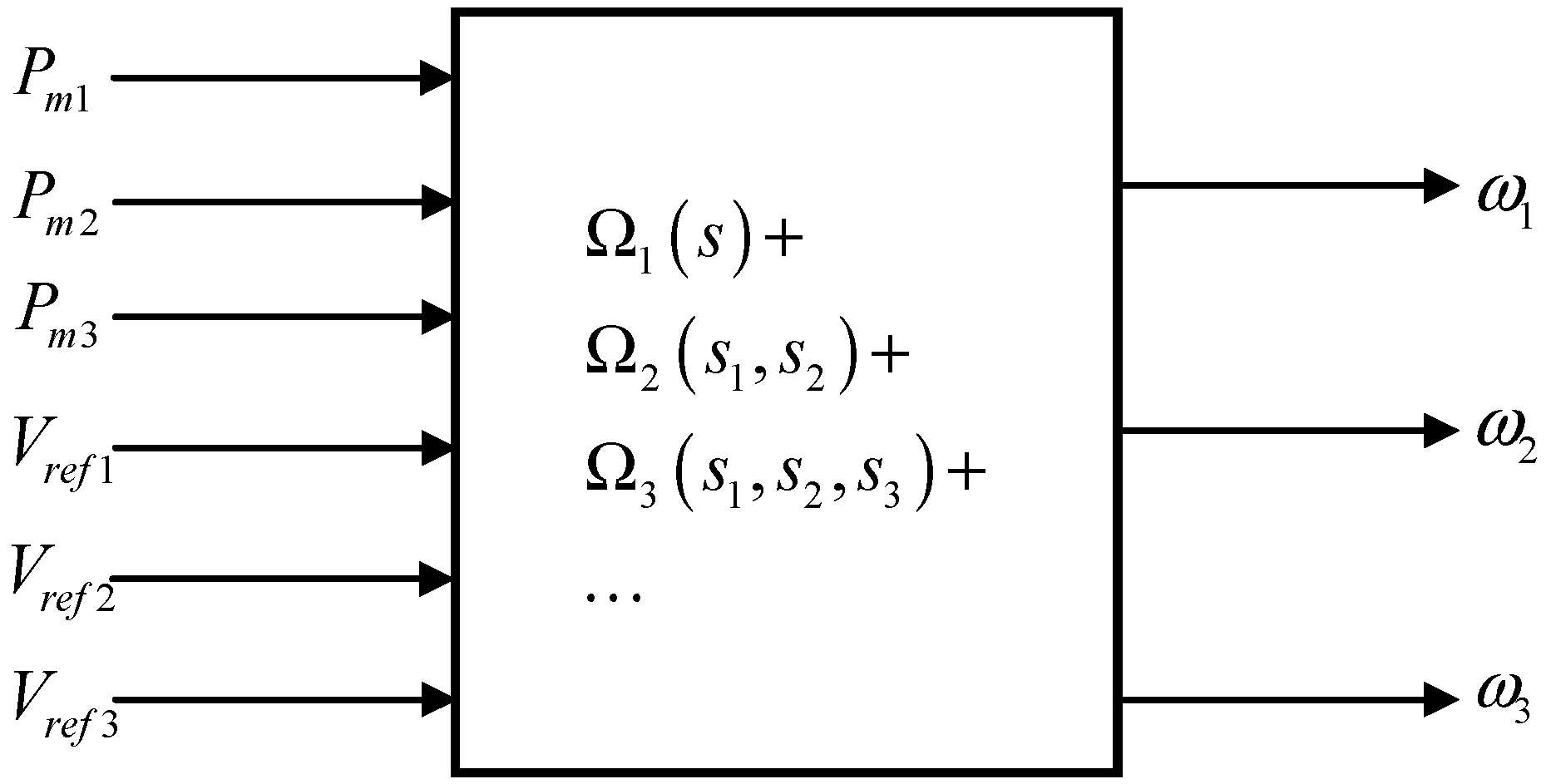
5.1. Three Synchronous Machine–Nine Buses Test Power System
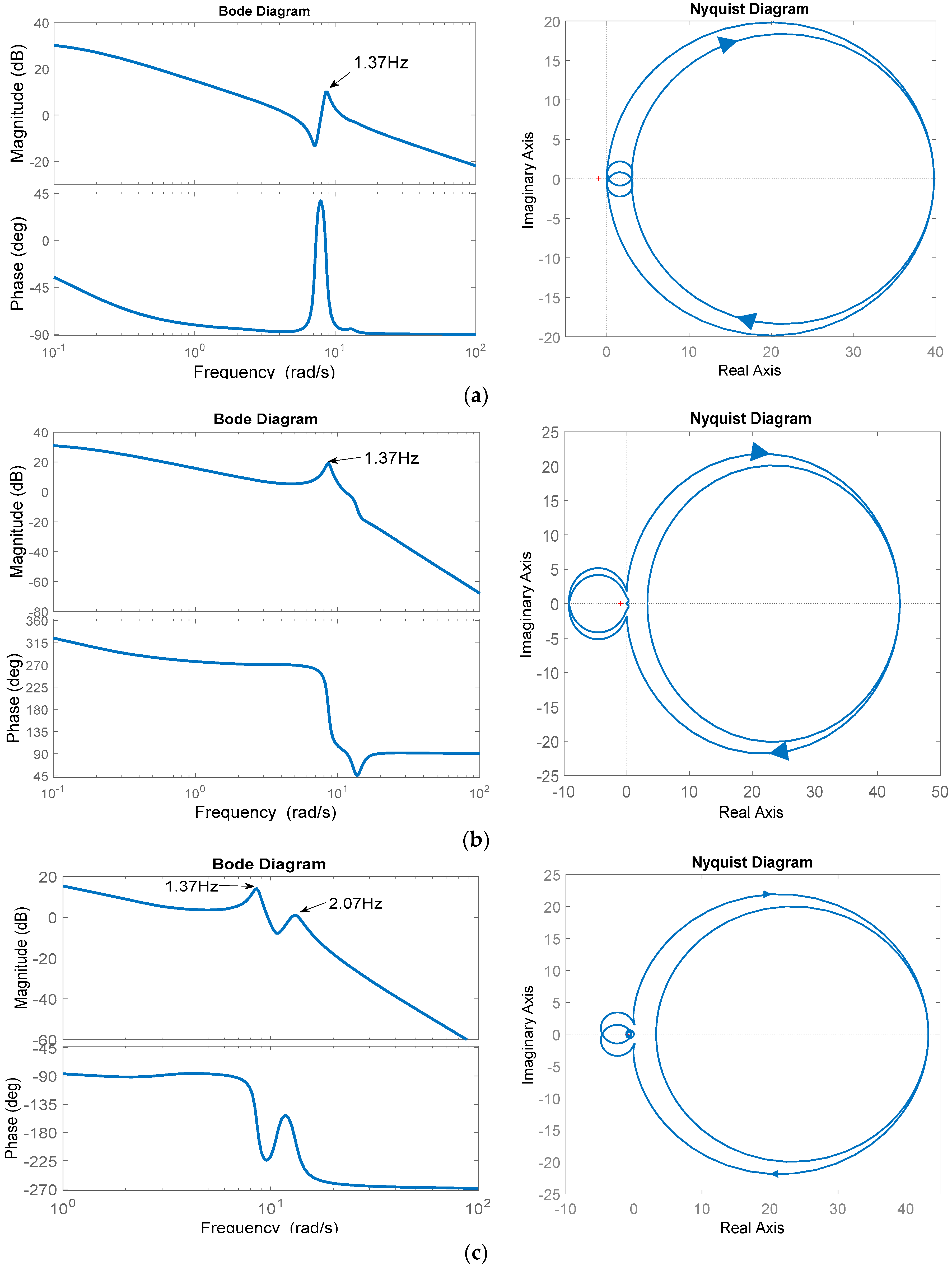
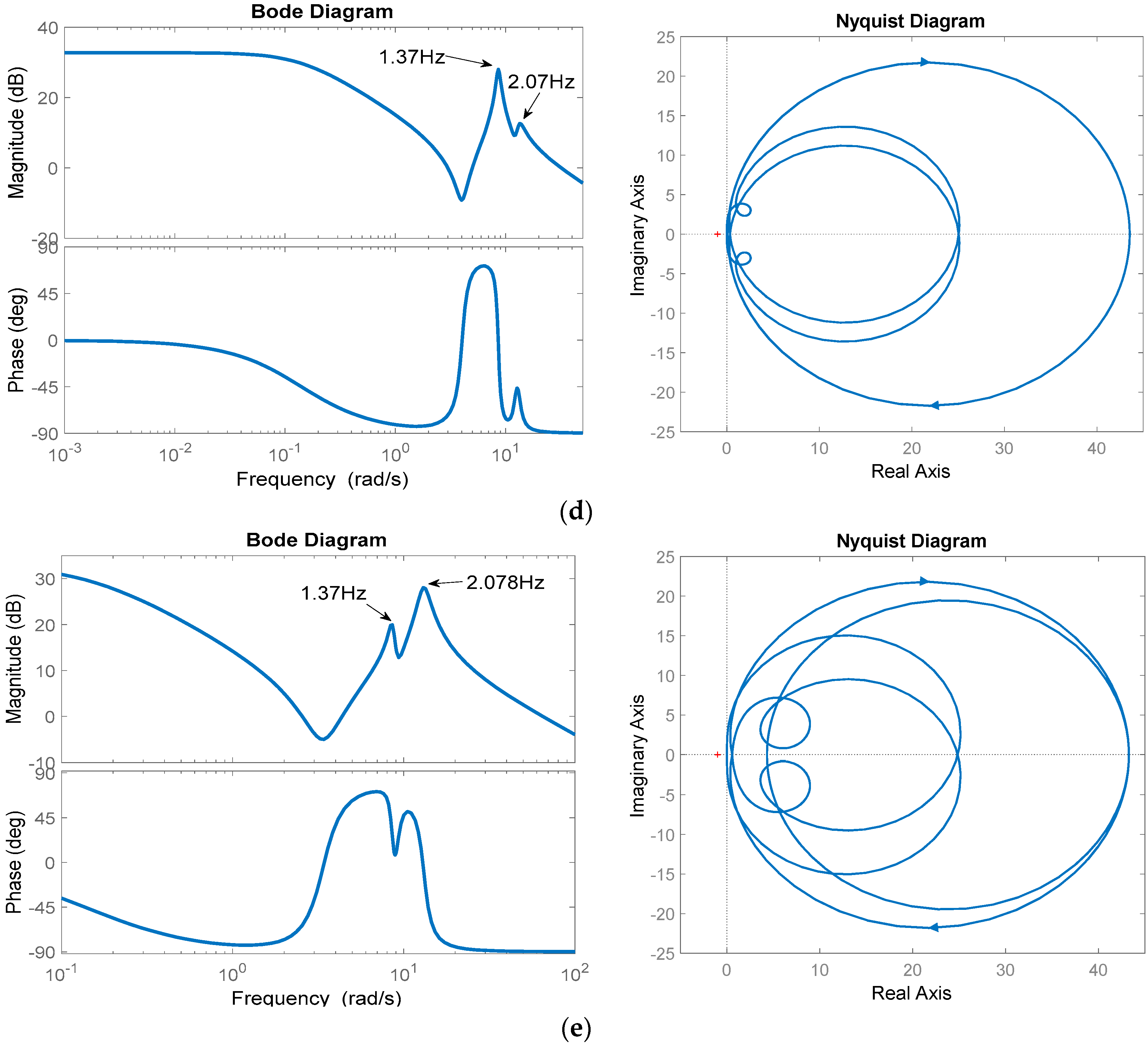
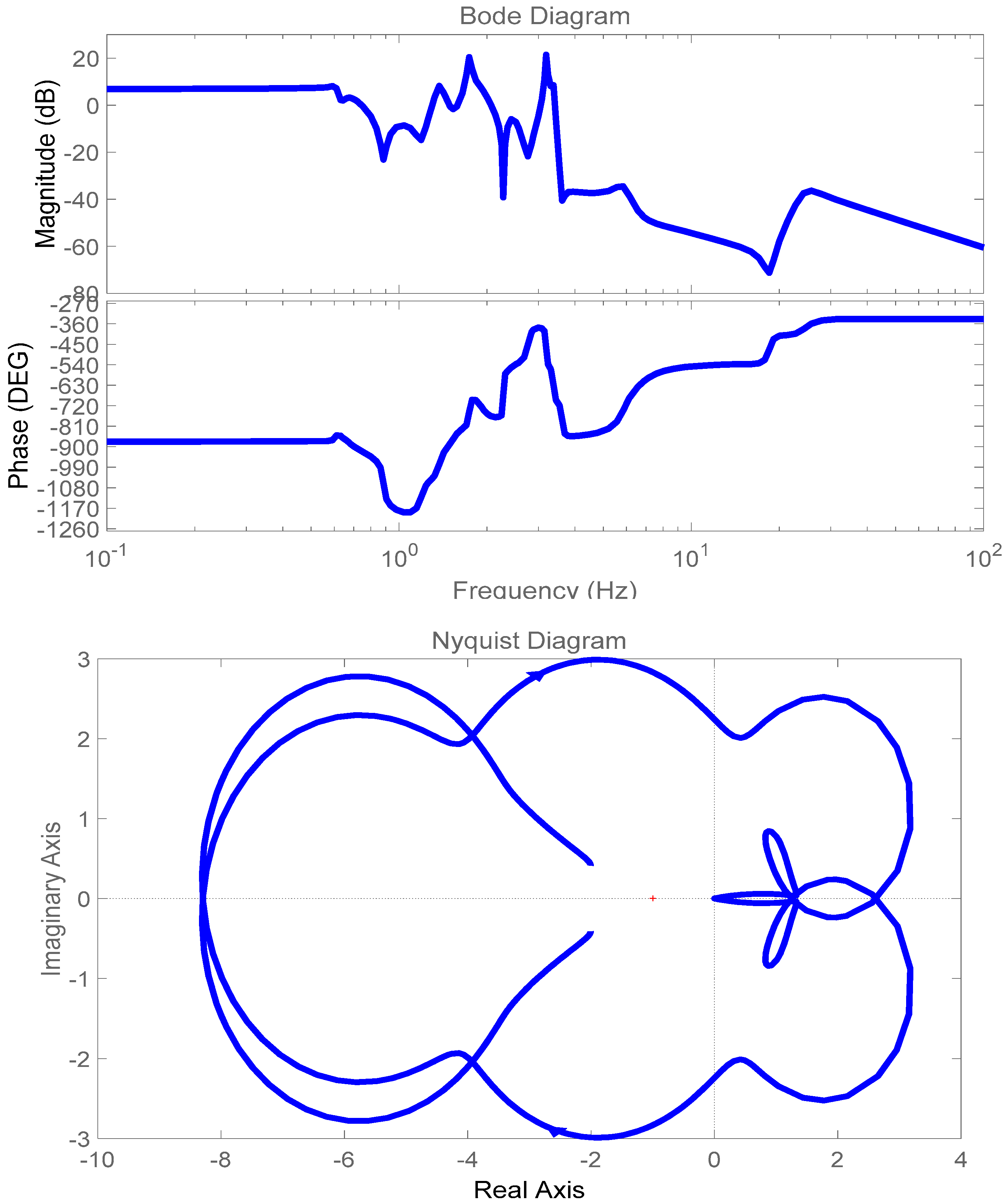
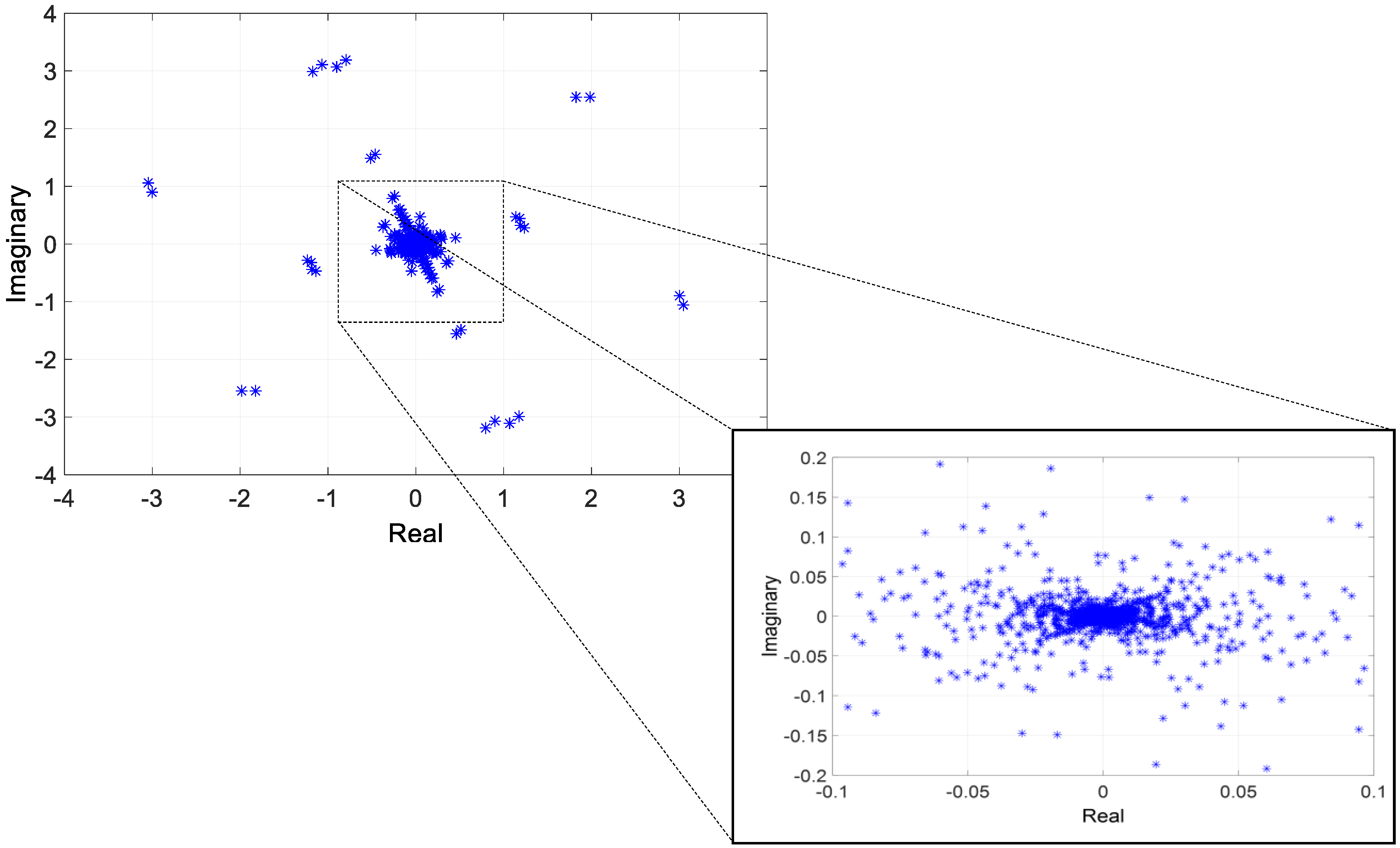
Nonlinear Transfer Functions
6. Conclusions
Author Contributions
Funding
Acknowledgments
Conflicts of Interest
Appendix A. Three Generators, Nine Buses Test Power System Data

| Sending Bus | Receiving Bus | Resistance | Reactance | Shunt Susceptance | Tap Ratio |
|---|---|---|---|---|---|
| 2 | 7 | 0 | 0.0625 | 0 | 1 |
| 7 | 8 | 0.0085 | 0.072 | 0.149 | 1 |
| 8 | 9 | 0.0119 | 0.1008 | 0.209 | 1 |
| 9 | 3 | 0 | 0.0586 | 0 | 1 |
| 9 | 6 | 0.039 | 0.17 | 0.358 | 1 |
| 6 | 4 | 0.017 | 0.092 | 0.158 | 1 |
| 4 | 5 | 0.01 | 0.085 | 0.176 | 1 |
| Gen | H | D | ||||||||
|---|---|---|---|---|---|---|---|---|---|---|
| G1 | 0.2 | 0 | 0.146 | 0.0608 | 8.96 | 0.0969 | 0.0608 | 0.31 | 23.64 | 0.0125 |
| G2 | 0.2 | 0 | 0.8958 | 0.1198 | 6 | 0.8645 | 0.1198 | 0.535 | 6.4 | 0.0068 |
| G3 | 0.2 | 0 | 1.3125 | 0.1813 | 5.89 | 1.2578 | 0.1813 | 0.6 | 3.01 | 0.0048 |
| Bus | ||||||
|---|---|---|---|---|---|---|
| 1 | 1.04 | 0 | 0.716 | 0.27 | 0 | 0 |
| 2 | 1.025 | 0.1623 | 1.63 | 0.067 | 0 | 0 |
| 3 | 1.025 | 0.082 | 0.85 | −0.109 | 0 | 0 |
| 4 | 1.026 | −0.0384 | 0 | 0 | 0 | 0 |
| 5 | 0.996 | −0.0698 | 0 | 0 | 1.25 | 0.5 |
| 6 | 1.013 | −0.0646 | 0 | 0 | 0.9 | 0.3 |
| 7 | 1.026 | 0.0646 | 0 | 0 | 0 | 0 |
| 8 | 1.016 | 0.0122 | 0 | 0 | 1 | 0.35 |
| 9 | 1.032 | 0.0349 | 0 | 0 | 0 | 0 |
References
- Dorf, R.C.; Bishop, R.H. Modern Control Systems, Pearson Education, 13th ed.; Addison-Wesley: Boston, MA, USA, 2016. [Google Scholar]
- Ogata, K. Modern Control Engineering; Prentice Hall: Upper Saddle River, NJ, USA, 1997. [Google Scholar]
- Vakilzadeh, M.; Eghtesad, M.; Vatankhah, R.; Mahmoodi, M. A Krylov subspace method based on multi-moment matching for model order reduction of large-scale second order bilinear systems. Appl. Math. Model. 2018, 60, 739–757. [Google Scholar] [CrossRef]
- Halás, M.; Kotta, U.; Moog, C.H. Transfer Function Approach to the Model Matching Problem of Nonlinear Systems. In Proceedings of the 17th World Congress International Federation of Automatic Control, Seoul, Korea, 6–11 July 2008; pp. 15197–15202. [Google Scholar]
- Martins, N.; Lima, L.T.G.; Pinto, H.J. Computing Dominant Poles of Power System Transfer Functions. IEEE Trans. Power Syst. 1996, 11, 162–170. [Google Scholar] [CrossRef]
- Martins, N.; Quintao, P.E. Computing Dominant Poles of Power System Multivariable Transfer Functions. IEEE Trans. Power Syst. 2003, 18, 152–159. [Google Scholar] [CrossRef]
- Rommes, J.; Martins, N. Efficient Computation of Transfer Function Dominant Poles Using Subspace Acceleration. IEEE Trans. Power Syst. 2006, 21, 1218–1226. [Google Scholar] [CrossRef]
- Rommes, J.; Martins, N. Efficient Computation of Multivariable Transfer Function Dominant Poles Using Subspace Acceleration. IEEE Trans. Power Syst. 2006, 21, 1471–1483. [Google Scholar] [CrossRef]
- Gomes, S., Jr.; Martins, N.; Portela, C. Sequential Computation of Transfer Function Dominant Poles of s-Domain System Models. IEEE Trans. Power Syst. 2009, 24, 776–784. [Google Scholar] [CrossRef]
- Varricchio, S.L.; Freitas, F.D.; Martins, N.; Véliz, F.C. Computation of Dominant Poles and Residue Matrices for Multivariable Transfer Functions of Infinite Power System Models. IEEE Trans. Power Syst. 2015, 30, 1131–1142. [Google Scholar] [CrossRef]
- Martins, N.; Pellanda, P.C.; Rommes, J. Computation of Transfer Function Dominant Zeros with Applications to Oscillation Damping Control of Large Power Systems. IEEE Trans. Power Syst. 2007, 22, 1657–1664. [Google Scholar] [CrossRef]
- Luntz, R.M. Approximate transfer functions for multivariable systems. Electron. Lett. 1970, 6, 444–445. [Google Scholar] [CrossRef]
- Smith, J.R.; Fatehi, F.; Woods, C.S.; Hauer, J.F.; Trudnowski, D.J. Transfer function identification in power system applications. IEEE Trans. Power Syst. 1993, 8, 1282–1290. [Google Scholar] [CrossRef]
- Zhang, J.; Moog, C.H.; Xia, X. Realization of Multivariable Nonlinear Systems Via the Approaches of Differential Forms and Differential Algebra. Kybernetika 2010, 46, 799–830. [Google Scholar]
- Halás, M.; Kotta, Ü. Realization problem of SISO nonlinear systems: A transfer function approach. In Proceedings of the 2009 IEEE International Conference on Control and Automation, Christchurch, New Zealand, 9–11 December 2009; pp. 546–551. [Google Scholar] [CrossRef]
- Kotta, Ü.; Zinober, A.S.I.; Liu, P. Transfer equivalence and realization of nonlinear higher order input–output difference equations. Automatica 2001, 37, 1771–1778. [Google Scholar] [CrossRef]
- Halás, M.; Kotta, Ü. Extension of the transfer function approach to the realization problem of nonlinear systems to discrete-time case. IFAC Proc. 2010, 43, 179–184. [Google Scholar] [CrossRef]
- Chua, L.O.; Ng, C.Y. Frequency-domain analysis of nonlinear systems: Formulation of transfer functions. IEE J. Electron. Circuits Syst. 1979, 3, 257–269. [Google Scholar] [CrossRef]
- Halás, M. An algebraic framework generalizing the concept of transfer functions to nonlinear systems. Automatica 2008, 44, 1181–1190. [Google Scholar] [CrossRef]
- Schoukens, M.; Tiels, K. Identification of block-oriented nonlinear systems starting from linear approximations: A survey. Automatica 2017, 85, 272–292. [Google Scholar] [CrossRef] [Green Version]
- Can, S.; Unal, A. Transfer Functions for Nonlinear Systems Via Fourier-Borel Transforms; IEEE International Symposium on Circuits and Systems: Espoo, Finland, 1988; Volume 3, pp. 2445–2448. [Google Scholar] [CrossRef]
- Cheng, C.M.; Peng, Z.K.; Zhang, W.M.; Meng, G. Volterra-series-based nonlinear system modeling and its engineering applications: A state-of-the-art review. Mech. Syst. Signal Process. Part A 2017, 87, 340–364. [Google Scholar] [CrossRef]
- Gomes, S., Jr.; Martins, N.; Portela, C. Modal Analysis Applied to s-Domain Models of AC Networks. IEEE Power Eng. Soc. Winter Meet. 2001, 3, 1305–1310. [Google Scholar]
- Pariz, N.; Schanechi, H.M.; Vaahedi, E. Explaining and Validating Stressed Power Systems Behavior Using Modal Series. IEEE Trans. Power Syst. 2003, 18, 778–785. [Google Scholar] [CrossRef]
- Shanechi, H.M.; Pariz, N.; Vaahedi, E. General Nonlinear Modal Representation of Large Scale Power Systems. IEEE Trans. Power Syst. 2003, 18, 1103–1109. [Google Scholar] [CrossRef]
- Rodríguez, O.; Medina, A.; Román-Messina, A.; Esquivel, C.R.F. The Modal Series Method and Multi-Dimensional Laplace Transforms for the Analysis of Nonlinear Effects in Power Systems Dynamics. In Proceedings of the IEEE General Meeting 2009, Calgary, AB, Canada, 26–30 July 2009. [Google Scholar]
- Rodriguez, O.; Medina, A. Systematic higher order nonlinear analysis of power systems operating under perturbation conditions. Electr. Eng. 2017, 99, 141–159. [Google Scholar] [CrossRef]
- Rodríguez, O.; Medina, A. Nonlinear transfer function based on forced response modal series analysis. In Proceedings of the 2011 North American Power Symposium, Boston, MA, USA, 4–6 August 2011; pp. 1–8. [Google Scholar] [CrossRef]
- Lubbock, J.K.; Bansal, V.S. Multidimensional Laplace Transforms for Solution of Nonlinear Equations. Proc. IEE 1969, 116, 2075–2082. [Google Scholar] [CrossRef]
- Mohler, R.R. Nonlinear Systems: Applications to Bilinear Control; Prentice Hall: Upper Saddle River, NJ, USA, 1991. [Google Scholar]
- Rugh, W.J. Nonlinear System Theory: The Volterra/Wiener Approach; The Johns Hopkins University Press: Baltimore, MD, USA, 1981. [Google Scholar]
- Pu, X.Z.; Zhu, M.W.; Fan, M.J. The Study of Dynamic Characteristics in Nonlinear Systems. IEEE Trans. Instrum. Meas. 1995, 44, 652–656. [Google Scholar]
- Trudnowski, D.J.; Smith, J.R.; Short, T.A.; Pierre, D.A. An Application of Prony Methods in PSS Design for Multimachine Systems. IEEE Trans. Power Sys. 1991, 6, 118–126. [Google Scholar] [CrossRef]
- Halás, M.; Kotta, Ü. Pseudo-Linear Algebra: A Powerful Tool in Unification of the Study of Nonlinear Control Systems. IFAC Proc. 2007, 40, 711–716. [Google Scholar] [CrossRef]
- Isidori, A. Nonlinear Control Systems: An Introduction, 2nd ed.; Springer: Berlin, Germany, 1989. [Google Scholar]
- Schetzen, M. The Volterra and Wiener Theories of Nonlinear Systems; John Wiley: New York, NY, USA, 1980. [Google Scholar]
- Busggang, J.J.; Ehrman, L.; Graham, J.W. Analysis of Nonlinear Systems with Multiple Inputs. Proc. IEEE 1974, 62, 1088–1119. [Google Scholar] [CrossRef]
- George, D.A. Continuous Nonlinear Systems; Technical Report 355; Massachusetts Institute of Technology, Research Laboratory of Electronics: Cambridge, MA, USA, 24 July 1959. [Google Scholar]
- Karmakar, S.B. Solution of Nonlinear Differential Equations by Using Volterra Series. Indian J. Pure Appl. Math. 1979, 10, 421–425. [Google Scholar]
- Kundur, P. Power System Stability and Control; McGraw-Hill: New York, NY, USA, 1994. [Google Scholar]
- Anderson, P.M.; Fouad, A.A. Power System Control, and Stability, 2nd ed.; John Wiley & Sons: Hoboken, NJ, USA, 2003. [Google Scholar]


| Residues | Poles | Frequency (Hz) | Damping Ratio | |
|---|---|---|---|---|
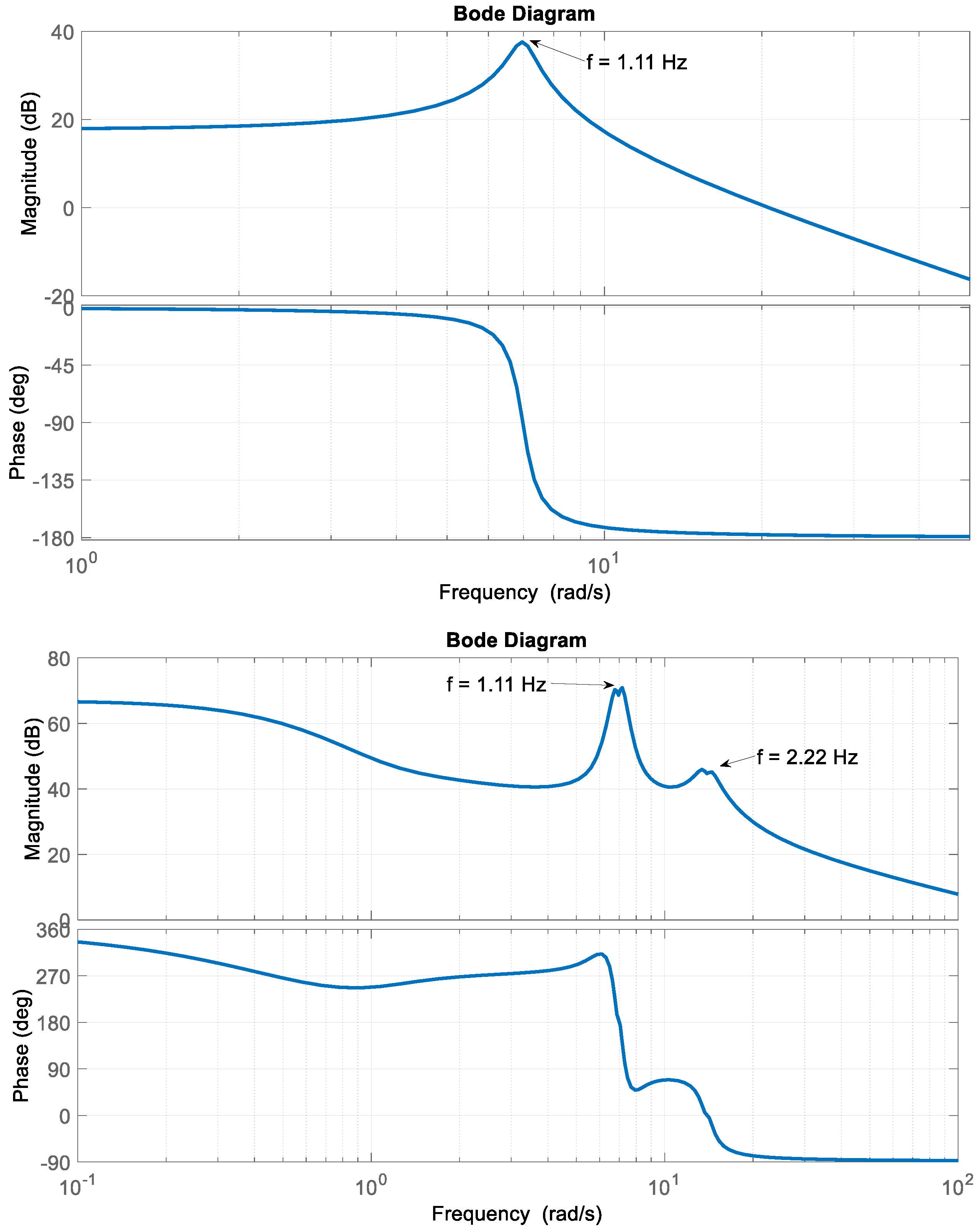
| First Order Transfer Function | −27.0380i | −0.3571 + 6.9715i | 1.1096 | 0.0512 |
| 27.0380i | −0.3571 − 6.9715i | −1.1096 | 0.0512 | |
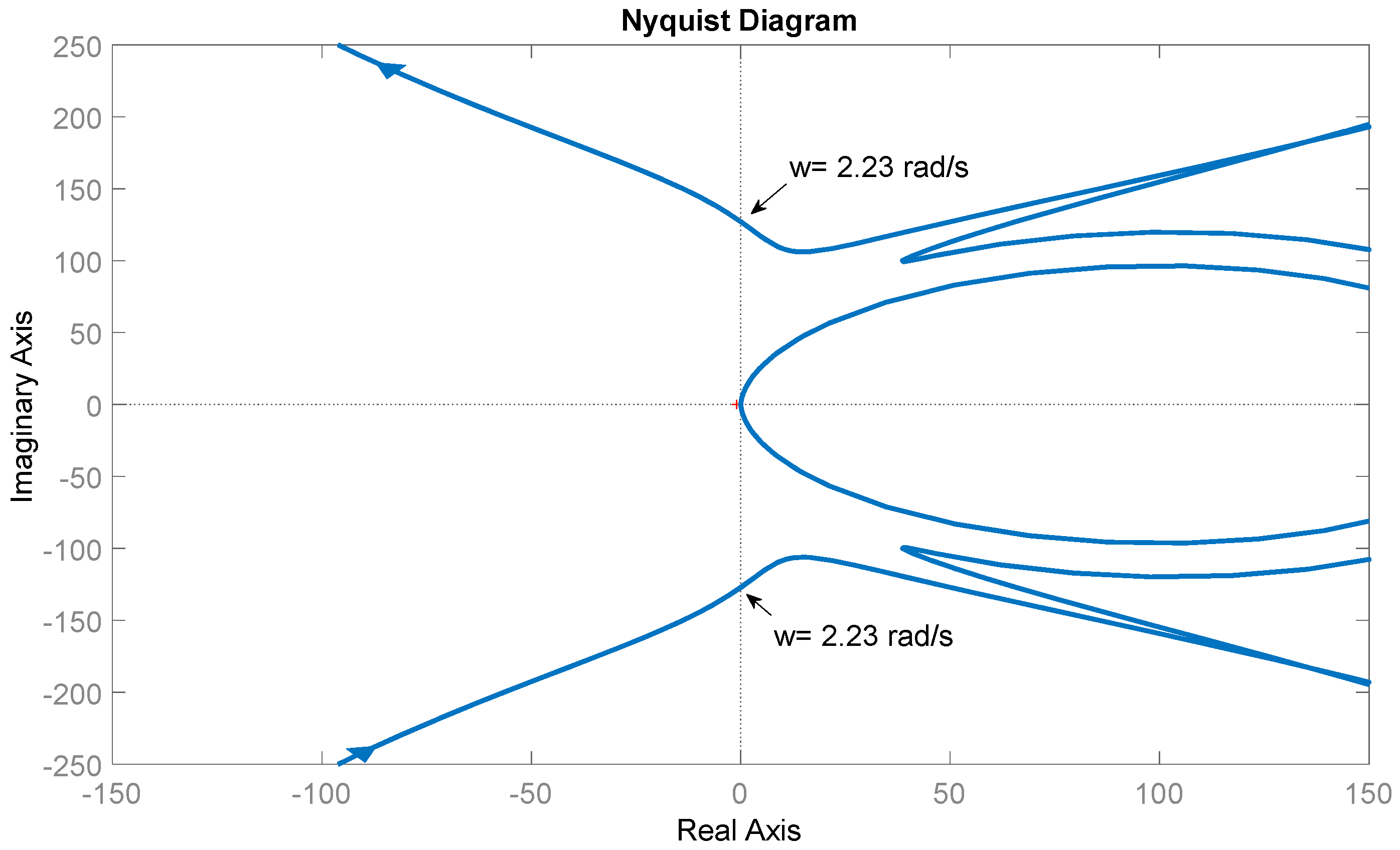
| Second Order Transfer Function | 223.24370479 − 11.4365329i | −0.7143 + 13.9430i | 2.2191 | 0.0512 |
| −223.24370479 + 11.4365329i | −0.3571 + 6.9715i | 1.1096 | 0.0512 | |
| 223.24370479 − 11.4365329i | −0.7143 | - | - | |
| −223.24370479 + 11.4365329i | −0.3571 + 6.9715i | 1.1096 | 0.0512 | |
| 223.24370479 − 11.4365329i | −0.7143 | - | - | |
| −223.24370479 + 11.4365329i | −0.3571 + 6.9715i | 1.1096 | 0.0512 | |
| −74.58811208 − 1.27368937i | −0.7143 − 13.9430i | 2.2191 | 0.0512 | |
| 74.58811208 + 1.27368937i | −0.3571 + 6.9715i | 1.1096 | 0.0512 | |
| −74.58811208 − 1.27368937i | −0.7143 + 13.9430i | 2.2191 | 0.0512 | |
| 74.58811208 + 1.27368937i | −0.3571 − 6.9715i | 1.1096 | 0.0512 | |
| 223.24370479 − 11.4365329i | −0.7143 | - | - | |
| −223.24370479 + 11.4365329i | −0.3571 − 6.9715i | 1.1096 | 0.0512 | |
| 223.24370479 − 11.4365329i | −0.7143 | - | - | |
| −223.24370479 + 11.4365329i | −0.3571 − 6.9715i | 1.1096 | 0.0512 | |
| 223.24370479 − 11.4365329i | −0.7143 −13.9430i | 2.2191 | 0.0512 | |
| −223.24370479 + 11.4365329i | −0.3571 − 6.9715i | 1.1096 | 0.0512 |
© 2019 by the authors. Licensee MDPI, Basel, Switzerland. This article is an open access article distributed under the terms and conditions of the Creative Commons Attribution (CC BY) license (http://creativecommons.org/licenses/by/4.0/).
Share and Cite
Rodríguez Villalón, O.; Medina-Rios, A. Transfer Function with Nonlinear Characteristics Definition Based on Multidimensional Laplace Transform and its Application to Forced Response Power Systems. Energies 2019, 12, 4061. https://doi.org/10.3390/en12214061
Rodríguez Villalón O, Medina-Rios A. Transfer Function with Nonlinear Characteristics Definition Based on Multidimensional Laplace Transform and its Application to Forced Response Power Systems. Energies. 2019; 12(21):4061. https://doi.org/10.3390/en12214061
Chicago/Turabian StyleRodríguez Villalón, Osvaldo, and Aurelio Medina-Rios. 2019. "Transfer Function with Nonlinear Characteristics Definition Based on Multidimensional Laplace Transform and its Application to Forced Response Power Systems" Energies 12, no. 21: 4061. https://doi.org/10.3390/en12214061