Abstract
A detailed numerical analysis of secondary flows in a transonic turbine is presented in this paper. The turbine stage is optimized by mitigating secondary flow through the method of non-axisymmetric endwall design. An automated optimization platform of NUMECA/Design3D was coupled with Euranus as a flow solver for the numerical investigation. The contoured endwalls of the stator and the rotor hub were designed based on equidistant Bézier curves along the camber line in the blade channel. The initial design samples were ten times the number of the design variables, and were generated through the LHS method for database generation. The optimization of the endwalls was achieved by using a state-of-the-art multi-objective optimization algorithm, NSGA-II, connected with the BPNN to increase the isentropic efficiency and decrease the secondary kinetic energy, while the mass flow and the degree of reaction were constrained to remain on the datum value as in the original geometry. The individual optimization of the hub endwalls of the stator and the rotor produced an increase in the efficiency of 0.27% and 0.25%, respectively, resulting in a cumulative improvement of 0.46% in the efficiency. The increase in the performance was analyzed at part-load conditions, and it was further confirmed through unsteady simulations.
1. Introduction
“Of all the fluid-dynamic devices invented by the human race, axial flow turbomachines are probably the most complicated.” This was aphoristically observed and narrated by Bradshaw [1]. The fluid flow brought about by the presence of endwalls in axial flow turbines is an important contributor to this complexity. According to Denton’s research, the endwall losses may contribute to one-third of the total losses in axial flow turbines [2]. The endwall losses are composed of endwall boundary layer dissipation and secondary flows. The secondary endwall losses arise from the viscous effects at the endwall and the pressure gradient [3]. These losses can be reduced by the active control method of boundary layer blowing [4], but the passive control method of three-dimensional non-axisymmetric endwall design is widely employed to manipulate the secondary flow in axial flow compressors and turbines.
Mitigation of secondary loss through endwall optimization of subsonic axial turbines has been a topic of interest for researchers for a couple of decades. However, the optimization of transonic axial turbines has not been investigated much, and less literature is available on the topic of non-axisymmetric endwall contouring for transonic stages.
This method was first presented by Rose, aiming for the attenuation of the circumferential non-uniformities and smoothing out the NGV pressure flow field so that the leakage of coolant from the disc rim seal could be reduced (to avoid hot gas ingestion). The flow field was very sensitive at Mach 1, and the endwall variations anticipated improved efficiency [5]. To exploit the potential for reducing secondary flow, a non-axisymmetric endwall was redesigned again for the rotor of a high-pressure axial turbine in a Durham linear cascade. It was determined that the secondary losses were related to endwall curvature. The profile had a convex curvature around the pressure surface to reduce the pressure there, and a concave curvature around the suction surface to increase the pressure there. This resulted in a reduction of the cross-pressure gradient, but the losses still increased slightly [6]. Later, the endwall curvature of the turbine rotor blade was designed with the help of an extended 3D linear design system that was already in practice for the forward and inverse design of turbine aerofoils. The CFD code used by Rolls-Royce predicted that the non-axisymmetric turbine endwall could narrow down the secondary kinetic energy, and in particular gas angle deviations at the exit, but the total reduction in loss was predicted to be small, because a counter-rotating (corner) vortex appeared for the final profiled endwall [7]. This CFD code of Rolls-Royce was based on the method described by Moore [8]. The potential of non-axisymmetric endwalls implied by the Durham Cascade results was validated through the Trent 500 HP Turbine under engine-representative conditions. The endwalls of the nozzle guide vane and the rotor were redesigned by using 0th-order and 1st-order harmonics with the design objective of minimization of the secondary kinetic energy helicity. The increase in total-to-total efficiency due to the nozzle guide vane was predicted to be 0.24%, and the rotor endwall design produced a 0.16% increment [9]. An intermediate pressure turbine (transonic) model rig of the Trent 500 engine was redesigned by applying non-axisymmetric endwalls to the vane and the blade, and this was tested in the presence of an upstream Trent 500 HP model turbine designed by Brennan et al. The overall improvement in the efficiency increased to 0.9% due to the redesign of the high pressure and intermediate pressure stages [10].
Poehler et al. numerically analyzed the impact of tangentially endwall contouring with the bowed first stator and the tangentially endwall contoured rotor of 1½ stage turbine. The endwall profiles were modified through an automatic optimization process with isentropic efficiency as a target function. Multiple optimized stator endwall designs resulted in an increase in stator total pressure loss, but the homogenized exit flow angles reduced the blade loading, thus overcompensating advantages in the rotor losses [11]. An automatic optimization setup of IsightTM (Dassault System, Waltham, MA, USA) grounded on the B-splines surface technique coupled with Ansys CFX (13.0, ANSYS Inc., Canonsburg, PA, USA) was used to optimize the hub and shroud the endwalls of the 1st stator and the rotor hub of the LISA turbine. This resulted in an increase in efficiency by 0.4% based on steady simulations and a mixing plane model, but the degree of reaction after the optimization was drastically increased to 12.5%, removing the benefits of actual performance enhancement [12]. The Multi-point Search-based Efficient Global Optimization (MSEGO) algorithm 3D blade parameterization, coupled with the RANS solver technique, was presented through knowledge-based design optimization of a typical low-aspect-ratio blade. The objective function consisted of mass flow averaged total pressure coefficient with constraints on mass flow and yaw angles. The optimized solution gave a pressure coefficient 0.49% higher than the datum design, but at the expense of a 1.59% increment in the mass flow because the concave surface of the endwall had increased the throat area [13].
In the other study, a non-axisymmetric hub was designed by cutting a circumferential groove through the hub endwall of the first stator of the 1.5 stage subsonic axial turbine. The groove parameters were controlled through the surrogate model in an automated computer-driven hub contouring technique formed by the application of OpenFOAM (3.2, The OpenFOAM Foundation, London, United Kingdom). The optimized surface predicted a reduction of the total pressure loss coefficient by 2.72% [14]. Rehman et al. presented a systematic optimization of the complete stage of the subsonic high-pressure turbine of an aero-engine through the method of non-axisymmetric endwall contouring. A pseudo-target function was set up to increase the isentropic efficiency while constraining the mass flow rate in an automatic optimization framework of FINE/Design3D (10.1, NUMECA International, Brussels, Belgium). The individually optimized stator and rotor predicted improvements in efficiency of 0.14% and 0.1%, respectively, and deterioration in the performance was avoided under off-design conditions [15].
In the case of a transonic high-pressure turbine, Kim at al. implemented a kriging-based approximation of the target function and optimized the stator endwalls through a genetic algorithm. The individual cases of the hub, the casing, and the combined optimization were formulated to study the secondary flows, and changes in efficiency of 0.13%, 0.40%, and 0.39%, respectively, were noticed. However, these were achieved at the expense of a mass flow rate constraint limit of 1.0% of the base value. This limit was greater, and any improvement in the performance could not be considered decisive. The constraint limit was even violated and increased the mass flow by 1.4% for the combined optimization case [16].
These motivational studies instigated the authors to investigate a transonic high-pressure turbine for 3D endwall contouring in more detail. For this purpose, the stator hub and the rotor hub of a transonic turbine were optimized individually in this paper. A multi-objective optimization methodology based on the back-propagation artificial network was implemented by using NSGA-II through the automatic optimization framework of FINE/Design3D. After the individual optimization of both rows, they were simulated together to gather the cumulative effect, and finally, the time-accurate simulations were carried out to authenticate our design.
2. Numerical Method
2.1. Transonic Turbine Test Case
The geometrical overview of the transonic turbine test case is shown in Figure 1.
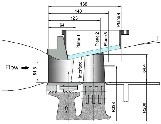
Figure 1.
Meridional flow path of the transonic turbine stage (Reproduced from [17]).
The stator upstream consisted of a convergent-divergent meridional path to accelerate the flow to supersonic velocity. This was achieved by contraction of the shroud contours, while the hub diameter remained constant in the stator section. The hub contour was cylindrical, while the shroud contour remained conical in the rotor section until the exit plane. Therefore, the inner diameter of the stage remained constant, which was exploited in this study to analyze the impact of non-axisymmetric endwall to minimize the secondary flows. The number of stator vanes was 24, and the number of rotor blades was 36, so the vane-blade ratio was 2:3. The tip clearance was 1.56% of the blade height at the leading edge. The absolute Mach number at the stator inlet and rotor inlet was about 0.14 and 1.12, respectively. The rotational speed was 10,600 revolutions per minute and the total pressure ratio was 3.5. For more detail specifications of this turbine and experimental data, please refer to the article [17].
2.2. Numerical Solver
Numerical simulations were performed using commercial software FINE/Turbo (10.1, NUMECA International, Brussels, Belgium). 3D steady compressible RANS were solved. The equations were discretized in space by cell-centered control volume technique, and in time by the explicit four-stage Runge-Kutta scheme. The multi-grid method was used to observe quick convergence. The SST turbulence model was selected to precisely evaluate the performance during the optimization process. This two-equation model is a blended model that follows the behavior of the Wilcox model close to the solid walls and that of model away from the boundary layer edges in the region of turbulence or free shear layers. It can effectively handle the adverse pressure gradients and flow separations [18]. Therefore, secondary flows can be better predicted with SST . This is a good trade-off between computational cost and accuracy.
2.3. Boundary Conditions
The flow was modeled as a perfect gas with constant specific heat. The dynamic viscosity was rated by Sutherland’s law. Based on the stator chord, Reynold’s number was set to 5.25 × 10⁶. The absolute total pressure (350 kPa) and the absolute total temperature (403 K) were applied to the inlet boundary. The flow direction was bounded to be axial in meridional path i.e., 0° peripheral. The average static pressure (100 kPa) was imposed at the outlet boundary. The inlet was placed at 2.06 times the stator vane axial chord, while the outlet was placed at 1.65 times the rotor blade axial chord based on the designed operating conditions [17]. The side surfaces were treated as periodic boundary conditions. The flow in turbomachines is usually very complex due to blade row interactions, because the rotor/stator interfaces are very close to the blade rows. This problem is more prominent in transonic turbines, because non-physical reflections of steady pressure waves may occur at the interface due to the shock waves. Non-reflecting, meaning that out-going waves should be allowed to exit the R/S interface without being reflected back in a non-physical manner and contaminate the solution. It is a steady-state condition in which the exact conservation of the mass flow, momentum, and energy are guaranteed. Therefore, in order to cater to the reflection of shock waves, the R/S interface was represented by 2D non-reflecting boundary condition [19,20]. Numerical averaging takes place at R/S interface and a smooth transition of all the parameters across the interface.
2.4. Grid Topology
The computation grid was generated by multi-grid optimization in AutoGrid5, which is a fully automated grid generation tool. The optimization was achieved using steady simulations; therefore, the computation domain was comprised of 1 stator and 1 rotor passage, as shown in Figure 2. It is worth mentioning that the secondary flows can be influenced by the presence of fillets and their shapes [21,22]. However, this study was focused on the mitigation of secondary flows due to non-axisymmetric endwalls; therefore, the presence of fillets was not accounted for.
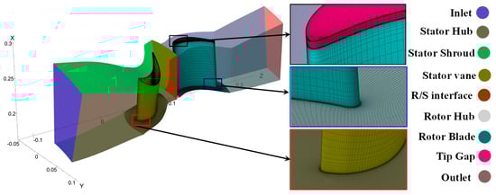
Figure 2.
Computational domain.
An O4H-topology was used in the blade passages. The inlet, outlet, and upper and lower blocks were of H-topology, while the skin block around the blade surface was given an O-topology (insets Figure 2) for the correct resolution of the boundary layer. The butterfly topology was adopted in the tip region. The mesh points were clustered close to the solid walls to have an appropriate grid resolution in the boundary layer. For this purpose, the mid-flow cells were confined to 30% of the total flow cells in the spanwise direction of the stator and the rotor. The distance between the first grid cell and the solid wall was selected to be 1.5 × 10⁻⁶ meters. The value of the non-dimensional parameter y+ was less than 3 in the first cell. This characteristic of the topology was kept constant for all simulations conducted during the grid dependency study, and the simulations of the optimization cycle. The combined number of mesh points of 4.17 million were selected after the grid dependency study as shown in Figure 3. Of approximately 4.17 million total cells, the stator and rotor comprised of 1.87 million and 2.3 million cells, respectively. The stator consisted of 69 cells in spanwise direction (X), 99 in pitchwise direction (Y) and 274 in azimuthal direction (Z), including the extended inlet portion, approximately. Similarly, the rotor consisted of 94, 99 and 221 cells in the X, Y and Z directions, respectively. The O-topology accounted for 41 cells in each row.
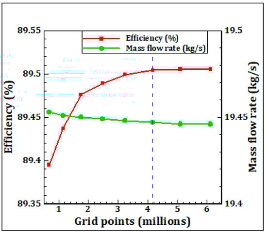
Figure 3.
Grid dependency: Plot of mass flow and efficiency.
The minimum value of skewness angle and the maximum value expansion ratio in the three-dimensional grid were kept less than 28° and 1.14, respectively, while the maximum value of the aspect ratio was 2200. The appearance of the mesh cells is shown in the inset of Figure 2. The root means square residual was 10−6 upon convergence for all the CFD calculations during grid dependency, and for the confirmation of optimized design. This value was less than 10−4 for the simulations of the optimization cycle. The computation expense of 1 typical steady simulation for the sixth-order convergence was approximately 120 min of wall clock time on 8 core machine of 2.6 GHz speed.
3. Optimization Framework
Before starting the optimization cycle, the fillets of the vane and the blade were removed, as this study was dedicated to understanding the effect of a non-axisymmetrical endwall on secondary flows. All steps of the flow diagram are shown in Figure 4.
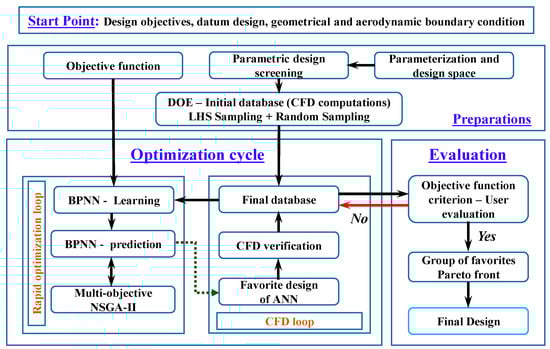
Figure 4.
Flow chart of the design optimization system.
The first task of parameterization in the “Preparation” box is elucidated in the following section. The parametric geometry, the control points, and the performance parameters defined for the optimization objective were fed to the environment of FINE/Design3D. The parametric geometry was screened for performance evaluation with respect to the original geometry and considered appropriate for the optimization cycle because it was a perfect replica of the original geometry.
The foundation of the optimization framework is the database with the results of all RANS computations performed during the design process. Before the optimization cycle begins, it is always necessary to have a sufficient number of samples to initialize the optimization process. In this study, the initial database was comprised of a combination of the samples generated through the Latin Hypercube Sampling (LHS) method and random sampling method. The number of initial samples was more than 10 times the number of control points of the stator hub and the rotor hub, and these were fed into the approximation model. Steady RANS were solved for each of the samples and converged solutions were stored in the database. To reduce the computational cost, the connection between the optimization target (objective function) and the initial database samples was established through some approximation model that replaced numerical simulations before the optimization cycle. BPNN was used as an approximation model because of the excellent capability of non-linear mappings which led to the best reproduction of initial samples contained in the database [23]. BPNN consists of two hidden layers in between the first layer containing the information of perturbed endwall geometry and the last layer containing the information of performance parameters. Using small random values, the weight and bias factors are initialized, and the information is passed to the next layer through a sigmoidal transfer function. Usually, the output vector provided by the network corresponds to the desired output vector in the forward training phase of BPNN iteration. The error between the real and desired value is back-propagated to the network input to adjust connecting weights and minimize the error. This process of updating weights is repeated for each training set until the weights converged in the backward process. This is why it is called a back-propagating neural network. BPNN in conjunction with the genetic algorithm was successfully used by Demeulenaere et al. for the formulation of single objective functions [24].
Therefore, BPNN predicted the approximate relationship between the design control variables and performance. The optimum solutions were found based on this relationship by using the optimization technique formed in NSGA-II, which was developed by Deb et al. [25]. The result of every design iteration was determined by solving three-dimensional steady RANS. The result of each iteration was inspected and anticipated to be in accordance with the criterion of the minimization of the objective function. NSGA-II is a multi-objective evolutionary algorithm and searches for a set of optimum solutions called a “Pareto set”. An individual dominates another individual if and only if the objectives of the former are better than the objective of the latter. The solutions that were not dominated by other solutions form the “Pareto front set”, and the best solution was selected from among these [26].
3.1. Endwall Profile Design Method and Design Space
The parameterization of the endwall is a very important step in an optimization procedure. This was carried out using ‘AutoBlade’, which is a parametric blade modeling tool. Endwalls can be designed in two ways. The first is that the endwall is controlled through curves in axial and pitchwise direction. In the second method, the endwall is generated by control points on the spline surface. In this paper, the second method was adopted because it had a high degree of freedom. Using this method, the parameterized area started upstream of the leading edges and ended downstream of the trailing edges of the stator and the rotor hub. The stator and the rotor blade channel were divided into 6 cuts, each with a distance of 20% of the blade channel width to the next one as shown in Figure 5a,b. The parametric domain was not allowed beyond the leading and trailing edges. In the circumferential direction, the perturbation law was defined by Bézier curves. Each curve consisted of 6 control points controlled by height variation in the radial direction, of which the points on the leading and the trailing edges were kept fixed to ensure continuity. The points were equally spaced between the leading and trailing edges of the stator and the rotor along the virtual streamlines as shown in Figure 5c. Therefore, 4 control points for every cut were automatically managed by the algorithm in the design space. The parametric model of the stator and the rotor, individually, consisted of 24 active free control points. For the optimization, the variation range of all parameters (24 points) was ±5 mm and ±6 mm in the vertical direction for the stator and rotor endwalls, respectively. This variation was equal to 10% of the span of the stator and the rotor, approximately.
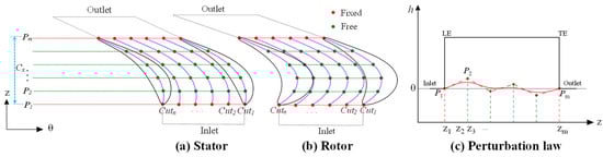
Figure 5.
(a–c) Control point distribution.
3.2. Objective Functions (Multi-Objective Problem Formulation)
A general form of the multi-objective optimization problem can be expressed as:
where stands for the objective functions. and represent the equality and inequality constraints with the total number of J and K, respectively. represents “n” number of design variables within lower and upper bounds.
In this study, two separate optimization problems were formulated. Each problem consisted of three objectives at a time in order to obtain a Pareto optimal solution. The design objectives were of conflicting nature in both formulations. In this study, the isentropic efficiency (η), and the degree of reaction (Ω) are defined as follows:
The secondary kinetic energy (SKE) is a parameter that indicates the strength of secondary loss. It has been fundamentally defined and thoroughly discussed by Vinuesa et al. [27]. This strength of secondary kinetic energy was defined in terms of the coefficient of secondary kinetic energy (CSKE) as follows:
This definition of CSKE is an effective representation of secondary kinetic energy, and this is consistent with the definition of Ingram [28]. The first optimization, called Opt_S, was set up for the performance enhancement by increasing η, decreasing CSKE while constraining the mass flow rate equal to the original design point value. The second optimization, called Opt_R, was set up for the performance enhancement by increasing η while maintaining the value of and Ω equal to the original design value. Here, Opt_S and Opt_R stand for the optimization of the endwall of the stator hub and the rotor hub, respectively.
4. Results and Analysis
4.1. Optimization Results
The results in terms of the variations of parameters involved in the formulation of the objective function are summarized in Table 1.

Table 1.
Summary of optimization results.
There was a noticeable improvement in the efficiency of both cases of optimization. For Opt_S, the overall value of CSKE was also decreased, and mass flow was marginally increased because it was not possible to attain the same mass flow due to variable curvature of endwall near the throat region. For Opt_R, the mass flow was exactly the same because the flow was already choked in the stator row, and the degree of reaction was dramatic but acceptable. This will be discussed in the next sections.
The configurations of the optimal designs are presented in Figure 6. Positive values of height variation in the radial direction depict convex curvature, while negative values represent concave curvature. The maximum and minimum values of the curvature variation were −2.62 mm and 1.62 mm for the stator hub endwall, and −1.73 mm and 2.21 mm for the rotor hub endwall. This showed that the spanwise curvature variation was not more than 50% of the allowable value confined in the optimizer. Therefore, the max/min curvature of the contoured endwalls varied by about 5% and 3.4% of the span of the stator and rotor, respectively. Another distinct feature of the curvature modifications was that the amplitude of the variation was more towards the trailing edges rather than the leading edges. The effect of this feature is presented in Figure 9 and Figure 14. The convex nature of the curvature acted to locally reduce the static pressure, on the contrary, the concave endwall curvature increased the local static pressure. This configuration helped to accelerate the pressure side leg of the horseshoe vortex near the pressure surface and retarded the development of the suction side leg, thus causing the pressure-side leg of the horseshoe vortex to interact further downstream of the suction surface. This delayed interaction reduced the strength of the fully developed passage vortex and is presented in Figure 11 and Figure 16. This will be further discussed in the next sections.
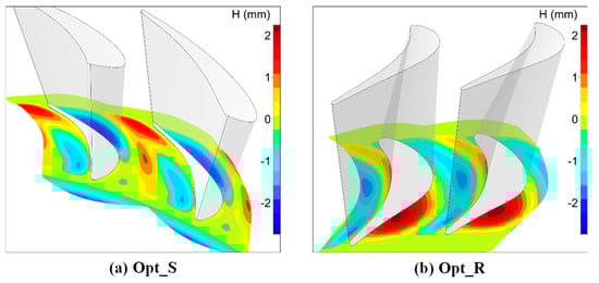
Figure 6.
(a,b) Endwall height variation in the radial direction of the optimal designs.
4.2. Optimization of the Stator Hub
The flow on the stator hub can be visualized by comparing limiting streamlines and the contours of static pressure for the axisymmetric and optimized cases. The pitchwise pressure gradient was reduced because the static pressure increased near the suction side, and the flow separation was avoided as shown by the ‘black circle’ reducing the intensity of the corner vortex as shown in Figure 7. Hence, the strength of cross-pitch flow was reduced.
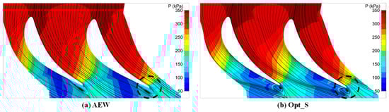
Figure 7.
(a,b) Limiting streamlines and static pressure contours at the stator hub.
As the efficiency and the secondary kinetic energy coefficient were included in the objective function, the radial distribution of these quantities is shown in Figure 8. The efficiency was improved to 60% of the blade span, indicating a strong impact of endwall optimization and reduction of secondary flow. The influence of the NEW was extended by approximately 10% from the hub. The reduction of the CSKE is used as a measure of the effectiveness of the endwall optimization [29]. Unlike subsonic turbines, CSKE was of a conflicting nature with the performance parameter of the efficiency. It decreased up to 15% of the blade span, but dramatically increased from 15% to 30% span, contributing less towards the overall decrease in the value of CSKE.
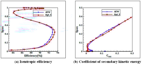
Figure 8.
Radial distribution of mass-averaged quantities: (a) at the exit; (b) at the interface.
The pressure distribution on the endwalls is reported in Figure 9 in terms of isentropic Mach number along the curvilinear abscissa of the stator vane. Mach number is defined as:
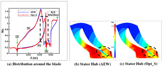
Figure 9.
(a–c) Isentropic Mach number distributions and contours at 1% span.
This supported the aforementioned interpretation of the effects of the optimization. The shape of the endwalls of AEW and Opt_S anticipated the flow acceleration from subsonic to transonic velocities by attaining sonic conditions on the suction side, but the occurrence of the shockwave was delayed for Opt_S, as shown in Figure 9a,c. For AEW, there was an early flow separation without reattachment at the stator vane trailing edge, as shown in Figure 9b. The shockwave was moved further downstream towards the TE due to the presence of a non-axisymmetric endwall, as shown by the dashed rectangular box in Figure 9a.
The investigation of the stator endwall was concluded upon the visualization of the entropy contours at different perpendicular planes through the stator passage with and without NEW, as shown in Figure 10. Only entropy contours above 30 J·kg−1·K−1 are shown. It can be seen that the highest values of entropy generation took place on the suction surface boundary layer, but this was only present over a small area, as shown by the ‘black square’. The decrease in entropy signatures indicated the reduction in the strength of the ‘loss core’ due to the modification in the suction side leg of the horseshoe vortex, as shown in Figure 10b.
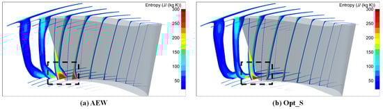
Figure 10.
(a,b) Entropy contours at equidistant cutting planes in a stator row.
The strength of secondary flows was further analyzed by the magnitude of streamwise vorticity. The streamwise vorticity is a projection of the total vorticity in a direction perpendicular to the flow. In this study, streamwise vorticity (ωs) is defined as:
The normalized form of the streamwise vorticity is defined as [30,31]:
where ωx and ωy are axial and tangential components of the streamwise vorticity, respectively. Figure 11 shows the contour plots of the normalized streamwise vorticity () at the exit of the stator (plane 1). The flood contours, along with limited isolines, showed that the passage vortex and counter vortex were obvious at plane 1. The passage vortex had vorticity with a negative sign, while the counter vortex had a positive sign. The negative vorticity extended towards the midspan region. The intensity of the predicted vortex cores decreased after the optimization, as indicated by the peak magnitudes of the contours. The dimensionless value of decreased by 24 and 29 for the passage and the counter vortices, respectively.
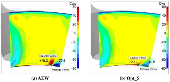
Figure 11.
(a,b) Contours of normalized streamwise vorticity.
4.3. Optimization of the Rotor Hub
As discussed in the previous section, the secondary flow losses are very sensitive to the blade loading. Figure 12 shows and compares pressure distribution along the blade surface at 1% and 50% span. Near the endwall at a 1% span, the increase in static pressure on the pressure surface near the leading edge was dramatic. Overall, the static pressure on the pressure surface remained unaltered, but the static pressure on the suction surface was increased compared to AEW, reflecting a decrease in the cross pressure gradient. Hence, the blade loading was reduced. The curve showing the pressure on the suction surface was also shifted further downstream towards the trailing edge, and the blade profile became typically aft-loaded, which was also an indication of the reduction of secondary loss as shown in Figure 12a. It was seen that the application of NEW had contributed less towards the reduction in blade loading at the midspan. The pressure on the suction surface was slightly increased, and there was no effect on the pressure surface as shown in Figure 12b. Any deteriorating effect of NEW was not noticed at the midspan in the region where the effects of boundary layer were minimum.
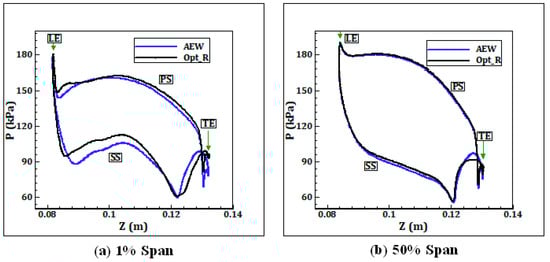
Figure 12.
(a,b) Distribution of static pressure on the rotor blade surface.
The efficiency and the degree of reaction were included in the objective function; therefore, the radial distribution of these quantities at the outlet of the rotor is shown in Figure 13. Likewise, the optimization results of the stator row, the efficiency was improved up to 60% of the blade span. Beyond 60% span, there was no influence of the NEW. When optimizing the turbine rotor, it is also important to keep the reaction of the rotor on the design value, not only the capacity. This is why, for the rotor optimization, the value of Ω was included in the objective function as a third objective. The value of Ω was also directly related to the flow angles at the outlet. The comparison of the two curves of AEW and Opt_R in Figure 13b shows that there was no variation of the degree of reaction along the span.
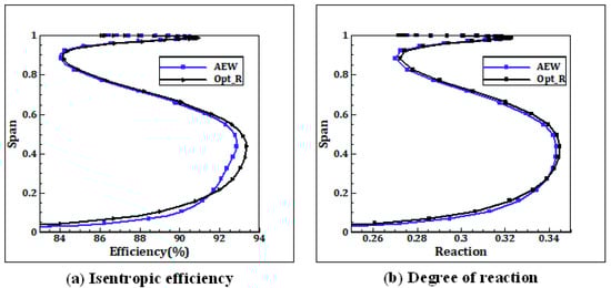
Figure 13.
(a,b) Spanwise distribution of mass-averaged quantities.
Corroborating the argument presented in Figure 12, the contours of Ma are additionally illustrated in Figure 14. There was a considerable redistribution of the contours of Mach number on the endwall near the suction surface. The shockwave had been removed as indicated by the ‘black oval’.
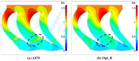
Figure 14.
(a,b) Contours of isentropic Mach number at the rotor hub.
The change in entropy at the outlet of the rotor is shown in Figure 15a,b. The combined effect of lower passage vortex and the stator wake are marked with the ‘black square’. The entropy generation was reduced as a result of a decrease in the strength of the vortices. Figure 15c,d shows the normalized helicity at the exit plane of the rotor, which is defined as:
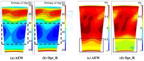
Figure 15.
(a–d) Comparisons of contours of entropy and helicity at the rotor exit.
and are the vectors of absolute velocity and absolute vorticity, respectively. The normalized helicity is the cosine of the angle between the velocity and vorticity vectors, reaches its highest absolute numbers in the vortex-core regions [32]. The sign of Hn indicates the direction of swirl (clockwise or counterclockwise) of the vortex with respect to the streamwise velocity component. The formation of contours showed an overall decrease in the strength of vortices. In particular, they were reduced towards the endwall of the rotor hub as shown by the ‘dotted rectangle’, as shown in Figure 15d.
4.4. Cumulative Effect of the Optimized Stator and Optimized Rotor
The stator and the rotor optimized endwalls were simulated together. The results met with an increment in the stage efficiency of 0.465% at the design point, as compared to the efficiency gained during individual optimization of the stator and the rotor of 0.27% and 0.25%, respectively. This showed that the performance of the turbine stage was not contaminated when both rows (stator and rotor) were simulated together. Figure 16 shows the turbine stage characteristics of entropy change and normalized streamwise vorticity in comparison with AEW at plane 3. For clarity, only contours for a 20% span were presented. The strength of the passage of vortex was reduced because the entropy was reduced by the value of 13 J·kg−1·K−1 in comparison with AEW as shown in Figure 16b. Similarly, the magnitude of the streamwise vorticity depicted that the passage and counter vortices were eradicated from the endwall.
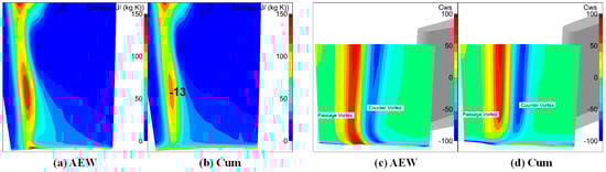
Figure 16.
(a–d) Comparisons of contours of entropy and helicity at plane 3.
The distribution of the static pressure on the suction surfaces of the stator and rotor along with the limiting streamlines are also shown in Figure 17. Inspecting the left figure, a distinct loss source in the form of corner vortex was clearly predicted and distinguished by the separation line. After the optimization, Opt_S, the trailing edge separation line and the corner vortex vanished completely. Moreover, the static pressure near the trailing edge of the stator increased, which was a typical indication that the profile had been aft-loaded. Similarly, the static pressure on the rotor suction surface decreased, especially from the leading edge to the mid chord. This helped to remove the separation line which was running from the rotor hub towards the midspan, as shown in Figure 17c.
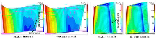
Figure 17.
(a–d) Static pressure contours superimposed with limiting streamlines.
4.5. Part Load Performance
Figure 18 compares the predicted stage efficiency from the axisymmetric (AEW) and non-axisymmetric (Cum) configuration at part load/off-design conditions. The optimized design point is the conditions under which the endwalls were designed in Section 4.2 and Section 4.3, and the term “Cum” refers to the cumulative effect of the optimization achieved in the aforementioned sections. The comparison was achieved by varying the outlet static pressure in the computational domain over the range of 100–225 kPa. Six discrete outlet conditions were simulated at progressively increasing the outlet static pressure which are presented by the dots in Figure 18. The inlet total pressure (350 kPa) and temperature (403 K) were kept fixed. The extreme of the curves on the right side showed that the chosen flow condition for the optimization was already a choking condition. Over the three part-load operating points on the right-hand side of Figure 18, the stage efficiency was more than the reference axisymmetric design. This improvement over the three operating points was consistent and of the same magnitude as that of a design point. However, the efficiency decreased for the two extreme part load conditions, as shown in the left-hand side of Figure 18. This is likely due to the increase in the capacity of the turbine at these two operating points.
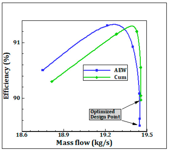
Figure 18.
Predicted stage efficiency with the axisymmetric and non-axisymmetric stator and rotor hub at design and off-design conditions.
4.6. Desing Confirmation through Unsteady Simulation
The flow around the turbine blade row is unsteady due to the relative motion between the stator/rotor domains. Therefore, the unsteady flow field of the axisymmetric and optimized turbine stage was numerically investigated by solving URANS using FINE/Turbo to access the impact of the steady assumptions taken into account during the optimization. The choice of the number of grid cells, the boundary conditions of the computation domain, and the turbulent model were kept the same as the steady analysis.
As there were 24 stator vanes and 36 rotor blades, the blade ratio between the stator vanes and the rotor blades was 2:3, a ratio which simplified the CFD model for unsteady simulations. Therefore, two stator vane and three rotor blade passages allowed us to compute only 1/12 of the row rings, and the stator/rotor interface was treated by the domain scaling method proposed by Rai [33,34].
Starting from the steady-state result as an input, the number of physical time steps was set to 120 for each cycle after the temporal sensitivity study. Every 5th time step was stored to get a resolution of 24 stored value-sets for the rotor passing. The value of Δt = 3.93 × 10⁻⁶ sec was calculated to obtain the periodic unsteady solution.
This calculation provided an angular resolution of 0.25° between each time step. This was fine enough to capture unsteady flow effects. One rotor period lasts 1440 time steps, and 100 inner iterations resulted in 144,000 time steps in total. Periodicity was evaluated by monitoring the variation of flow quantities over three consecutive periods. Generally, after the initial transients had been discarded, the unsteady solution was supposed to converge when global parameters like efficiency and mass flow rate started fluctuating periodically.
The comparison of the efficiency fluctuation is reported in Figure 19. The fluctuation has six peaks and six troughs in three periods. The time-averaged values of the efficiencies showed that the stage efficiency increased by 0.328% due to the cumulative effect of the optimization of both rows of the stator and the rotor. The efficiency after the optimization was higher than the original configuration in each physical time step. The result further suggested that the unsteady interaction between the stator and the rotor decreased due to the profiled endwalls but to a lesser extent, because the fluctuation magnitude of the efficiency decreased by the profiled endwalls.
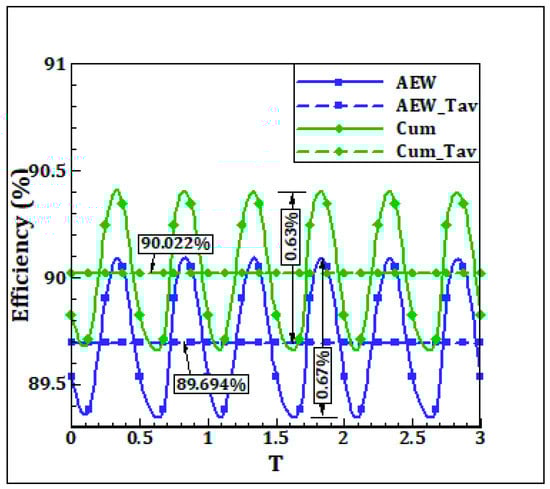
Figure 19.
Efficiency fluctuation at the different physical time.
The transport process of the passage vortex at different axial planes downstream of the rotor over one period is shown in Figure 20. The passage vortex is depicted in the form of time-resolved entropy contours. Four instants (t/T 0.00, 0.25, 0.50, 0.75) are presented to explain the change in entropy with respect to the rotor exit flow. The movement of one rotor period corresponds to turning of 10°; however, Figure 20 presents flow field over three rotor periods that corresponds to 30°. The unsteady rotor downstream flow field consisted of the rotor wake, and the tip-leakage and passage vortices. All these secondary flow features move with the rotor blade, but their strengths were time-varying. The tip leakage flow was not the domain of this study. The rotor passage vortex transported from plane 2 to the exit plane as shown by a black arrow. With respect to the unsteady simulation “Cum”, it could be seen that the passage vortex reduced its strength because the signature of entropy contours was diminished for all instances of time as shown in plane 4. This passage vortex of less intensity was still present at the exit plane of the computational domain for AEW. However, the unsteady simulations “Cum” showed that the passage vortex was completely resolved at the exit plane. The tip leakage vortex and the passage vortex was connected by the rotor wake. The rotor wake was clearly visible at t/T = 0.25 and t/T = 0.50 as shown by the ‘dashed ellipse’. The resolution of the rotor wake was also a noticeable change after the optimization.
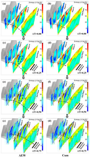
Figure 20.
(a–f) Time-resolved entropy contours at three different planes downstream of the rotor.
Lastly, averaging over the whole passing period T led to the visualization of the entropy contours as shown in Figure 21. Due to the same color bar, this figure can be compared to the time-resolved results of Figure 20. The dashed rectangle on plane 3 showed that the passage vortex reduced its strength.
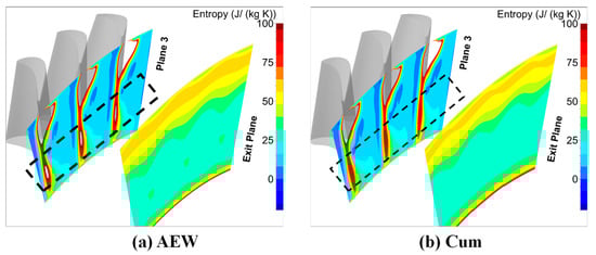
Figure 21.
(a,b) Time-averaged result of entropy contours at two planes downstream of the rotor.
5. Conclusions
Two separate non-axisymmetric endwalls for a transonic turbine stage, named Opt_S for the stator hub and Opt_R for the rotor hub, were designed and numerically investigated using NUMECA/Desing3D. The endwall was parameterized using Bézier curves formed through the control point distribution technique. The optimization was accomplished using function approximation and multi-objective NSGA-II algorithm coupled with RANS. Three objectives were defined for both the cases. Based on the analysis presented, the following conclusions were drawn.
- The optimization of the stator hub resulted in an increase in efficiency by 0.27%. The objective function was formulated based on the efficiency, mass flow rate and the coefficient of secondary kinetic energy. The mass flow rate was effectively controlled within the acceptable limit. The coefficient of the secondary kinetic energy was reduced by up to 4.92%. The radial distribution of the efficiency confirmed the performance improvement by up to 60%, while that of CSKE was convincing near the hub, but dramatic near the midspan region. The shockwave interaction with the suction surface was moved further downstream towards the trailing edge, and the flow separation was removed. The strength of the fully developed passage vortex in the stator was reduced by 32%, quantified in terms of the streamwise vorticity.
- The optimization of the rotor hub was also formulated based on the three objectives. The degree of the reaction was included in the objective function in place of CSKE. The efficiency was increased by 0.25%, while the mass flow rate remained constant. The radial distribution of the degree of reaction showed a good agreement with the performance improvement. The contours of the entropy, the streamwise vorticity and the normalized helicity at the exit of the rotor reflected a decrease in the strength of vortices. The flow separation line on the suction surface of the rotor which was emanating from the hub and running towards the mid-span was wiped out due to contouring. This also indicated the delay in the interaction of the pressure and suction side legs of the passage vortex.
Both cases of the optimization resulted in a significant improvement in the performance based on steady computations. The design of the endwalls was confirmed through unsteady simulations (URANS). The entropy decreased at different instances of time. The global performance was in agreement with optimization under steady conditions.
Author Contributions
B.L. put forward the idea and supervised the research work. A.R. conducted the simulation, the optimization and drafted the manuscript. M.A.A. visualized the results. All authors discussed the results and reviewed the manuscript.
Funding
This research received no external funding.
Acknowledgments
The authors would like to thank the Institute of Thermal Turbomachinery and Machine Dynamics, TU Graz; for providing the stage geometry upon request via email.
Conflicts of Interest
The authors declare no conflict of interest.
Nomenclature
| P | Pressure |
| t | Time |
| T | Temperature |
| T | Rotor blade passing period |
| V | Absolute velocity |
| y+ | Non-dimensional wall distance |
| Abbreviations | |
| AEW | Axisymmetric Endwall |
| BPNN | Back Propagation Neural Network |
| CFD | Computational Fluid Dynamics |
| Cum | Cumulative |
| LE | Leading Edge |
| NEW | Non-Axisymmetric Endwall |
| NSGA-II | Non-Dominated Sorting Genetic Algorithm II |
| Opt_S | Optimization of the stator hub |
| Opt_R | Optimization of the rotor hub |
| PS | Pressure Side |
| RANS | Reynolds-Average Navier-Stokes |
| SS | Suction Side |
| TE | Trailing Edge |
| URANS | Unsteady Reynolds-Average Navier-Stokes |
| Greek Symbols | |
| σ | Mass-averaged flow angle in both pitchwise and spanwise direction |
| γ | The ratio of Specific Heats |
| ρ | Density |
| Subscripts | |
| 0 | Stator Inlet |
| 1 | Stator/Rotor Interface |
| 2 | Rotor Outlet |
| R | Radial |
| sec | Secondary |
| t | Total |
| ta | tangential |
| z | Axial |
References
- Bradshaw, P. Turbulence modeling with application to turbomachinery. Prog. Aerospace. Sci. 1996, 32, 575–624. [Google Scholar] [CrossRef]
- Denton, J.D. The 1993 IGTI Scholar Lecture: Loss Mechanisms in Turbomachines. J. Turbomach. 1993, 115, 621–656. [Google Scholar] [CrossRef]
- Langston, L.S. Secondary Flows in Axial Turbines-A Review. Ann. N. Y. Acad. Sci. 2010, 934, 11–26. [Google Scholar] [CrossRef] [PubMed]
- Scheugenpflug, H.; Fottner, L. Performance Improvements of Compressor Cascades by Controlling the Profile and Sidewall Boundary Layers. J. Turbomach. 1992, 114, 477. [Google Scholar] [CrossRef]
- Rose, M.G. Non-axisymmetric endwall profiling in the HP NGV’s of an axial flow gas turbine. In Proceedings of the ASME 1994 International Gas Turbine and Aeroengine Congress and Exposition, The Hague, The Netherlands, 13–16 June 1994; American Society of Mechanical Engineers: New York, NY, USA, 1994. [Google Scholar]
- Hartland, J.; Gregory-Smith, D.; Rose, M. Non-axisymmetric endwall profiling in a turbine rotor blade. In Proceedings of the ASME 1998 International Gas Turbine and Aeroengine Congress and Exhibition, Stockholm, Sweden, 2–5 June 1998; American Society of Mechanical Engineers: New York, NY, USA, 1998. [Google Scholar]
- Harvey, N.W.; Rose, M.G.; Taylor, M.D.; Shahpar, S.; Hartland, J.; Gregory-Smith, D.G. Nonaxisymmetric turbine end wall design: Part I—Three-dimensional linear design system. J. Turbomach. 2000, 122, 278–285. [Google Scholar] [CrossRef]
- Moore, J.G. Calculation of 3-D flow without numerical mixing. In AGARDS 3D Computation Tech. Applied to Internal Flows in Propulsion Systems; NASA: Washington, DC, USA, 1985; pp. 8.1–8.14. [Google Scholar]
- Brennan, G.; Harvey, N.W.; Rose, M.G.; Fomison, N.; Taylor, M.D. Improving the Efficiency of the Trent 500-HP Turbine Using Nonaxisymmetric End Walls—Part I: Turbine Design. J. Turbomach. 2003, 125, 497–504. [Google Scholar] [CrossRef]
- Harvey, N.; Brennan, G.; Newman, D.; Rose, M. Improving turbine efficiency using non-axisymmetric end walls: Validation in the multi-row environment and with low aspect ratio blading. In Proceedings of the ASME Turbo Expo 2002: Power for Land, Sea, and Air, Amsterdam, The Netherlands, 3–6 June 2002; American Society of Mechanical Engineers: New York, NY, USA, 2002; pp. 119–126. [Google Scholar]
- Poehler, T.; Niewoehner, J.; Jeschke, P.; Guendogdu, Y. Investigation of Nonaxisymmetric Endwall Contouring and Three-Dimensional Airfoil Design in a 1.5-Stage Axial Turbine—Part I: Design and Novel Numerical Analysis Method. J. Turbomach. 2015, 137, 081009–081009-11. [Google Scholar] [CrossRef]
- Tang, H.; Liu, S.; Luo, H. Design optimization of profiled endwall in a high work turbine. In Proceedings of the ASME Turbo Expo 2014: Turbine Technical Conference and Exposition, Düsseldorf, Germany, 16–20 June 2014; American Society of Mechanical Engineers: New York, NY, USA, 2014. [Google Scholar]
- Song, L.; Guo, Z.; Li, J.; Feng, Z. Optimization and Knowledge Discovery of a Three-Dimensional Parameterized Vane with Nonaxisymmetric Endwall. J. Propuls. Power 2017, 34, 234–246. [Google Scholar] [CrossRef]
- Obaida, H.M.; Rona, A.; Gostelow, J.P. Loss Reduction in a 1.5 Stage Axial Turbine by Computer-Driven Stator Hub Contouring. J. Turbomach. 2019, 141, 061009. [Google Scholar] [CrossRef]
- Rehman, A.; Liu, B. Numerical Investigation and Non-Axisymmetric Endwall Profiling of a Turbine Stage. J. Therm. Sci. 2019, 28, 811–825. [Google Scholar] [CrossRef]
- Kim, I.; Kim, J.; Cho, J.; Kang, Y.-S. Non-axisymmetric endwall profile optimization of a high-pressure transonic turbine using approximation model. In Proceedings of the ASME Turbo Expo 2016: Turbomachinery Technical Conference and Exposition, Seoul, Korea, 13–17 June 2016; American Society of Mechanical Engineers: New York, NY, USA, 2016. [Google Scholar]
- Göttlich, E.; Neumayer, F.; Woisetschläger, J.; Sanz, W.; Heitmeir, F. Investigation of Stator-Rotor Interaction in a Transonic Turbine Stage Using Laser Doppler Velocimetry and Pneumatic Probes. J. Turbomach. 2004, 126, 297–305. [Google Scholar] [CrossRef]
- Menter, F.R. Two-equation eddy-viscosity turbulence models for engineering applications. AIAA J. 1994, 32, 1598–1605. [Google Scholar] [CrossRef]
- Giles, M.B. Stator/rotor interaction in a transonic turbine. J. Propuls. Power 1990, 6, 621–627. [Google Scholar] [CrossRef]
- Giles, M. UNSFLO: A Numerical Method for Unsteady Inviscid Flow in Turbomachinery; Gas Turbine Laboratory, Massachusetts Institute of Technology: Cambridge, MA, USA, 1988. [Google Scholar]
- Hawes, C.; Williams, R.; Ingram, G. Investigating endwall-blade fillet radius variation to reduce secondary flow losses. In Proceedings of the 11th European Conference on Turbomachinery: Fluid Dynamics and Thermodynamics, Madrid, Spain, 23–25 March 2015; European Turbomachinery Society: Florence, Italy, 2015. [Google Scholar]
- Ananthakrishnan, K.; Govardhan, M. Influence of fillet shapes on secondary flow field in a transonic axial flow turbine stage. Aerosp. Sci. Technol. 2018, 82, 425–437. [Google Scholar] [CrossRef]
- Pierret, S.; Van den Braembussche, R.A. Turbomachinery Blade Design Using a Navier–Stokes Solver and Artificial Neural Network. J. Turbomach. 1999, 121, 326–332. [Google Scholar] [CrossRef]
- Demeulenaere, A.; Ligout, A.; Hirsch, C. Application of multipoint optimization to the design of turbomachinery blades. In Proceedings of the ASME Turbo Expo 2004: Power for Land, Sea, and Air, Vienna, Austria, 14–17 June 2004; American Society of Mechanical Engineers: New York, NY, USA, 2004; pp. 1481–1489. [Google Scholar]
- Deb, K.; Pratap, A.; Agarwal, S.; Meyarivan, T. A fast and elitist multiobjective genetic algorithm: NSGA-II. IEEE T. Evolut. Comput. 2002, 6, 182–197. [Google Scholar] [CrossRef]
- Wang, X.; Hirsch, C.; Kang, S.; Lacor, C. Multi-objective optimization of turbomachinery using improved NSGA-II and approximation model. Comput. Method Appl. Mech. Eng. 2011, 200, 883–895. [Google Scholar] [CrossRef]
- Vinuesa, R.; Schlatter, P.; Nagib, H. Secondary flow in turbulent ducts with increasing aspect ratio. Phys. Rev. Fluids 2018, 3, 054606. [Google Scholar] [CrossRef]
- Ingram, G.L. Endwall Profiling for the Reduction of Secondary Flow in Turbines. PhD Thesis, University of Durham, Durham, England, 2003. [Google Scholar]
- Snedden, G.; Dunn, D.; Ingram, G. On-and off-design performance of a model rotating turbine with non-axisymmetric endwall contouring and a comparison to cascade data. Aeronat. J. 2018, 122, 646–665. [Google Scholar] [CrossRef]
- Zhu, C.; Wang, T.; Wu, J. Numerical Investigation of Passive Vortex Generators on a Wind Turbine Airfoil Undergoing Pitch Oscillations. Energies 2019, 12, 654. [Google Scholar] [CrossRef]
- Zorić, T. Experimental Investigation of Secondary Flows in a Family of Three Highly Loaded Low-Pressure Turbine Cascades; Carleton University: Ottawa, ON, Canada, 2006. [Google Scholar]
- Degani, D.; Seginer, A.; Levy, Y. Graphical visualization of vortical flows by means of helicity. AIAA J. 2012, 28, 1347–1352. [Google Scholar] [CrossRef]
- Rai, M.M. Three-dimensional Navier-Stokes simulations of turbine rotor-stator interaction. Part I-Methodology. J. Propuls. Power 1989, 5, 305–311. [Google Scholar] [CrossRef]
- NUMECA International. FINETM/Turbo 10.1—User Manual. NUMECA International: Brussels, Belgium, 2015. [Google Scholar]


© 2019 by the authors. Licensee MDPI, Basel, Switzerland. This article is an open access article distributed under the terms and conditions of the Creative Commons Attribution (CC BY) license (http://creativecommons.org/licenses/by/4.0/).