Article

A Simplified Numerical Model for the Prediction of Wake Interaction in Multiple Wind Turbines

Department of Mechanical Engineering, Kunsan National University, Gunsan 54150, Korea
*
Author to whom correspondence should be addressed.
Energies 2019, 12(21), 4122; https://doi.org/10.3390/en12214122
Submission received: 18 September 2019 / Revised: 19 October 2019 / Accepted: 23 October 2019 / Published: 29 October 2019
(This article belongs to the Section A3: Wind, Wave and Tidal Energy)

Abstract

:
In the design of wind energy farms, the loss of power should be seriously considered for the second wind turbine located inside the wake region of the first one. The rotation of the first wind-front rotor generates a high-vorticity wake with turbulence, and a suitable model is required in computational fluid dynamics (CFD) to predict the deficit of energy of the second turbine for the given configuration. A simplified numerical model based on the classical momentum theory is proposed in this study for multiple wind turbines, which is proposed with a couple of tuning parameters applied to Reynolds-averaged Navier-Stokes (RANS) analysis, resulting in a remarkable reduction of computational load compared with advanced methods, such as large eddy simulation (LES) where two parameters reflect on axial and rotational wake motion, simply tuned with the wind-tunnel test and its corresponding LES result. As a lumped parameter for the figure of merit, we regard the normalized efficiency on the kinetic power output of computational domain, which should be directed to maximize for the optimization of wind farms. The parameter surface is plotted in a dimensionless form versus intervals between turbines, and a simple correlation is obtained for a given hub height of 70% diameter and a fixed rotational speed tuned from the experimental data in a wide range.

1. Introduction

It has been established that the wake of a turbine degrades the performance of second ones, which should be seriously considered in the design process of a wind farm [1]. According to the recent literature [2,3] there have been various kinds of approaches for this problem: analytic models [4,5,6,7,8,9], numerical analyses [10,11,12,13,14,15,16,17], and experiment with wind tunnel [13,18,19] or on-site tests [20]. Thus far, many kinds of wake models have been introduced [4], but the velocity profile in the wake is still impossible to visualize easily due to the spiral tip vortex and turbulence with high vorticity, and the unsteady flow and the yaw error also make this problem more difficult [3,21]. The analytical models often use statistical Gaussian distributions in the wake, for example [8]. However, this cannot explain the fluid-dynamical physics lying in these phenomena. Other models also require some induced or parasite aerodynamic coefficients such as rotor thrust coefficient [4,8], which should be obtained from experiment in advance. Although there are many kinds of options in theories, its application to the real wind farms seems very difficult.
The recent development of high-performance computation has made it possible to do precise simulations on very complex turbulent flow around a rotational wind turbine with advanced numerical techniques such as LES (large eddy simulation) and DNS (direct numerical simulation). Therefore, computational fluid dynamics (CFD) is a kind of feasible method for terrain-coupled problems [10] or especially interactions of vortices in the wake region of turbines [11]. However, the computational load becomes so heavy that 24 million grids and 20-CPU cluster machine are used in the parallel processing [10], for instance, because LES generally requires much heavier load than Reynolds-averaged Navier-Stokes (RANS) simulations.
In this paper, we aim to develop a reliable and economic method that is a semi-analytical CFD model whose resultant correlations that can be easily used in the field of wind power industry. Two independent input parameters, based on momentum theory, are tuned with a wind tunnel test and LES data for a scaled model, which is extended to a wake-interaction problem by a simple superposition of boundary condition with RANS CFD. A parametric study is done to obtain a correlation for a wide range, validated with a real turbine array in an existing wind farm.

2. Implementation of the Numerical Model

In this section, we elucidate some key ideas to develop a simplified numerical model for the wake flow of a wind turbine [22]. The wake model for a rotor will be extended with a simple superposition to see the interaction with the next rotor.

2.1. Classical Momentum Theory

In the wake region of a turbine, Figure 1a, the rotation of flow, or the tip vortex filament is affected by the tangential component of wind speed, and the stream tube is expanded because the incident wind subtracts the kinetic energy to the rotor. With the application of classical momentum theory [1], the axial induction factor ( a ) is defined as the ratio of flow-velocity decrease relative to the incident wind speed ( U ), and the wind speed through the disk plane (2–3) is ( 1 a ) U .
η 1 = 1 a
where η 1 is regarded as the axial efficiency of rotor blade. The ideal value of a is calculated as 1/3 in Betz’s limit, but η 1 > 2 / 3 in real cases due to some additional losses. However, η 1 can depend on various conditions such as tip speed ratio, turbulence intensity, and other configuration variables, etc. Then the axial angular speed of wake ( ω ) is expressed as:
ω = 2 a η 2 Ω
where η 2 is the rotational efficiency of wake, and Ω is the angular speed of rotor. In the classical actuator disk theory considering the wake rotation, η 2 = 1 is generally used, but the effect of rotor rotation is limited in reality as η 2 < 1 from effects like the dissipation of turbulent flow.
Referred from Figure 1 in the simple actuator disk theory, the pressure difference just before and after the disk plane is derived with Bernoulli’s equation as follows:
p 2 p 3 = 1 2 ρ ( U 1 2 U 4 2 )
where U 4 = U 1 ( 1 2 a ) , and U 1 = U (free-stream flow velocity). Equation (3) is simply expressed as:
p 2 p 3 = 2 a ( 1 a ) ρ U 2
In the ideal HAWT (horizontal axis wind turbine), the rotational wake flow passes through the wind turbine, accelerating the angular speed from Ω to Ω + ω in the frame of inertia coordinate system. Here Ω is the angular speed of rotor while ω is the additional rotation of wake. Thus, the whole rotational effects are included in the following equation:
p 2 + 1 2 ρ [ U 2 ( 1 a ) 2 + Ω 2 r 2 ] = p 3 + 1 2 ρ [ U 2 ( 1 a ) 2 + ( Ω + ω ) 2 r 2 ]
p 2 p 3 = ρ ( Ω + 1 2 ω ) ω r 2
where the rotational induction factor a is defined from Equation (2) as, setting η 2 = 1 :
a = ω 2 Ω
Using Equation (7), Equation (6) is rewritten as:
p 2 p 3 = 2 a ( 1 + a ) ρ Ω 2 r 2
Equating Equations (4) and (8), the following equation is derived:
a ( 1 a ) a ( 1 + a ) = Ω 2 r 2 U 2
where the local speed ratio, defined as λ r = Ω r / U , and a in Equation (7) is obtained as the solution of the following quadratic equation:
a 2 + a a ( 1 a ) λ r 2 = 0
Equation (10) has generally two real solutions, but the positive value is selected since it is physically proper.
a = 1 2 + 1 2 [ 1 + 4 λ r 2 a ( 1 a ) ] > 0
From Equation (11), a is a function of axial induction factor a and the parameter λ r that is a function of radial position, r . However, a singularity for the infinite value of a occurs when r = 0 (at the center of rotor) in Equation (11), which is aphysical. Therefore, at the region of 10% rotor radius, the induction factor is set to a constant finite value, satisfying the continuity with limitation: refer to Figure 1b.
a = { 1 2 + 1 2 [ 1 + ( 20 λ ) 2 a ( 1 a ) ]    ,   r / R 0.1 1 2 + 1 2 [ 1 + ( 2 R λ r ) 2 a ( 1 a ) ]    ,   r / R > 0.1

2.2. CFD Model: Single Turbine

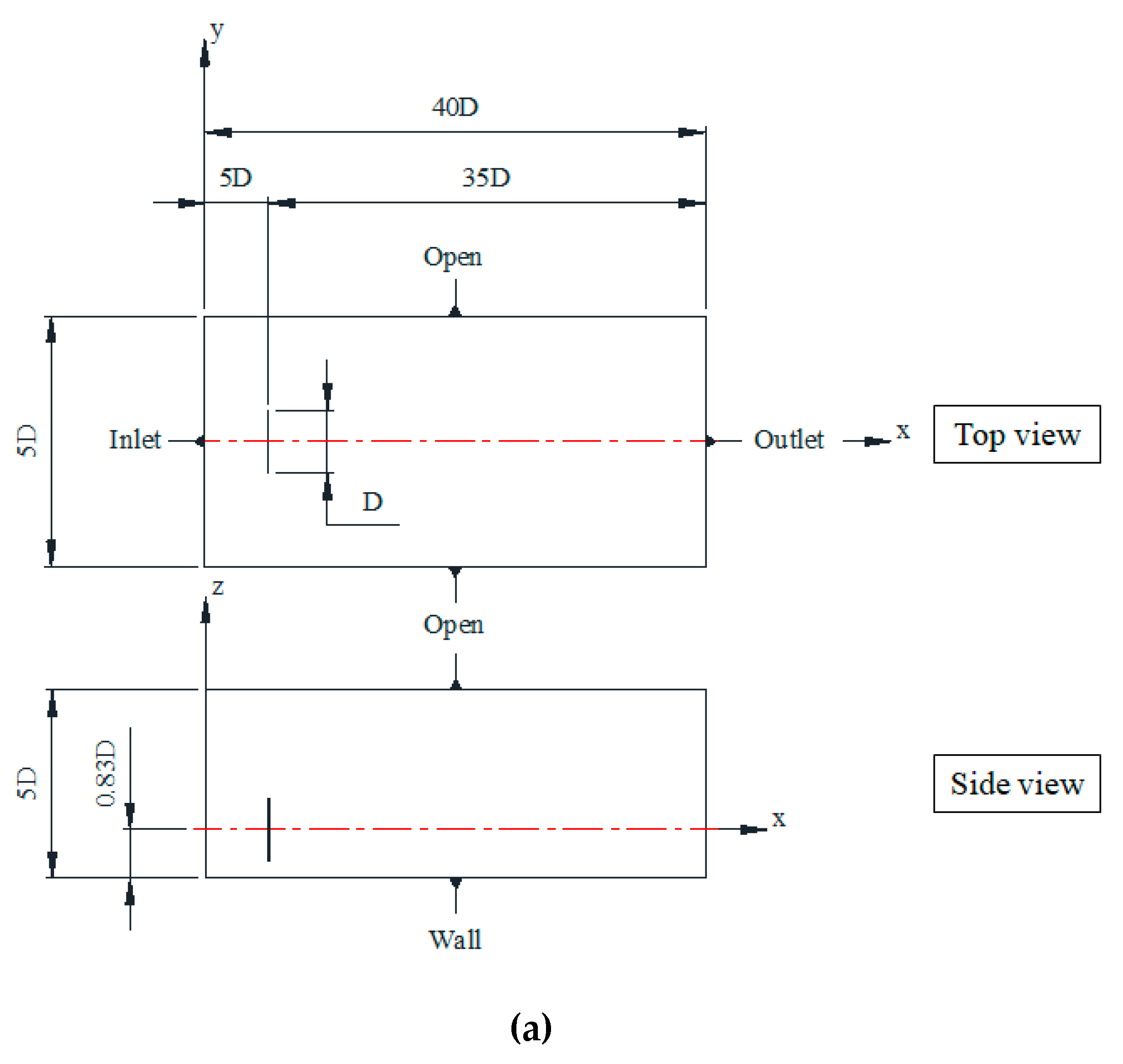
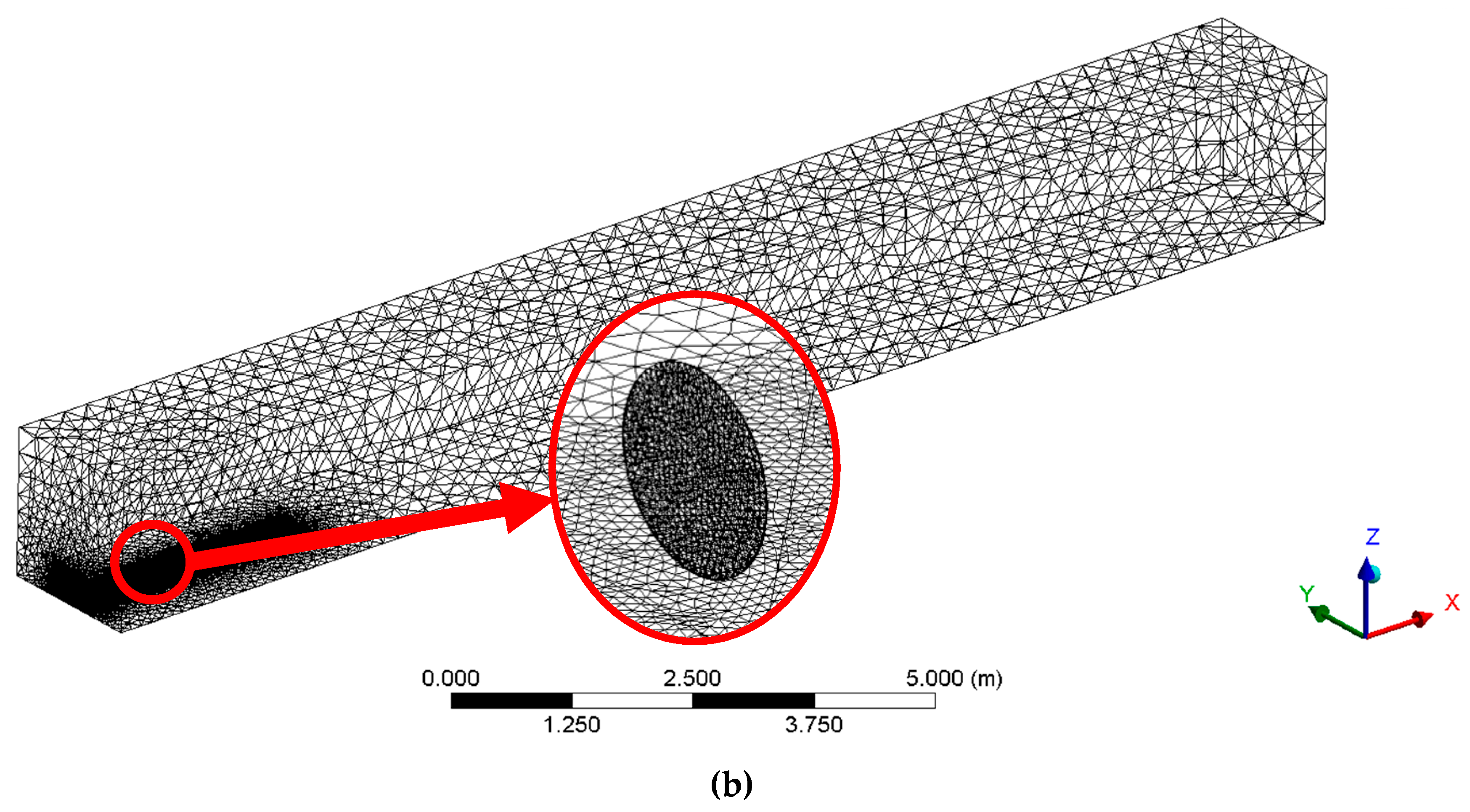
We used the wind tunnel test data of a single rotor blade and their LES result [14] for the tuning of parameters η 1 and η 2 . The basic performance of the rotor used in the experiment is given in Table 1, and the computational domain for CFD (computational fluid dynamics) is shown as Figure 2a. The grids are also presented is Figure 2b where the total numbers of elements are about 8 million (7,833,775), and to capture the complex flow phenomena at the wake region, the width three times the disk diameter is focused to concentrate meshes since the cross-sectional area of stream tube is double of the disk area in the ideal momentum theory.
The inlet velocity with turbulent boundary layer is given as the following profile:
U U = ( z H ) 1 7
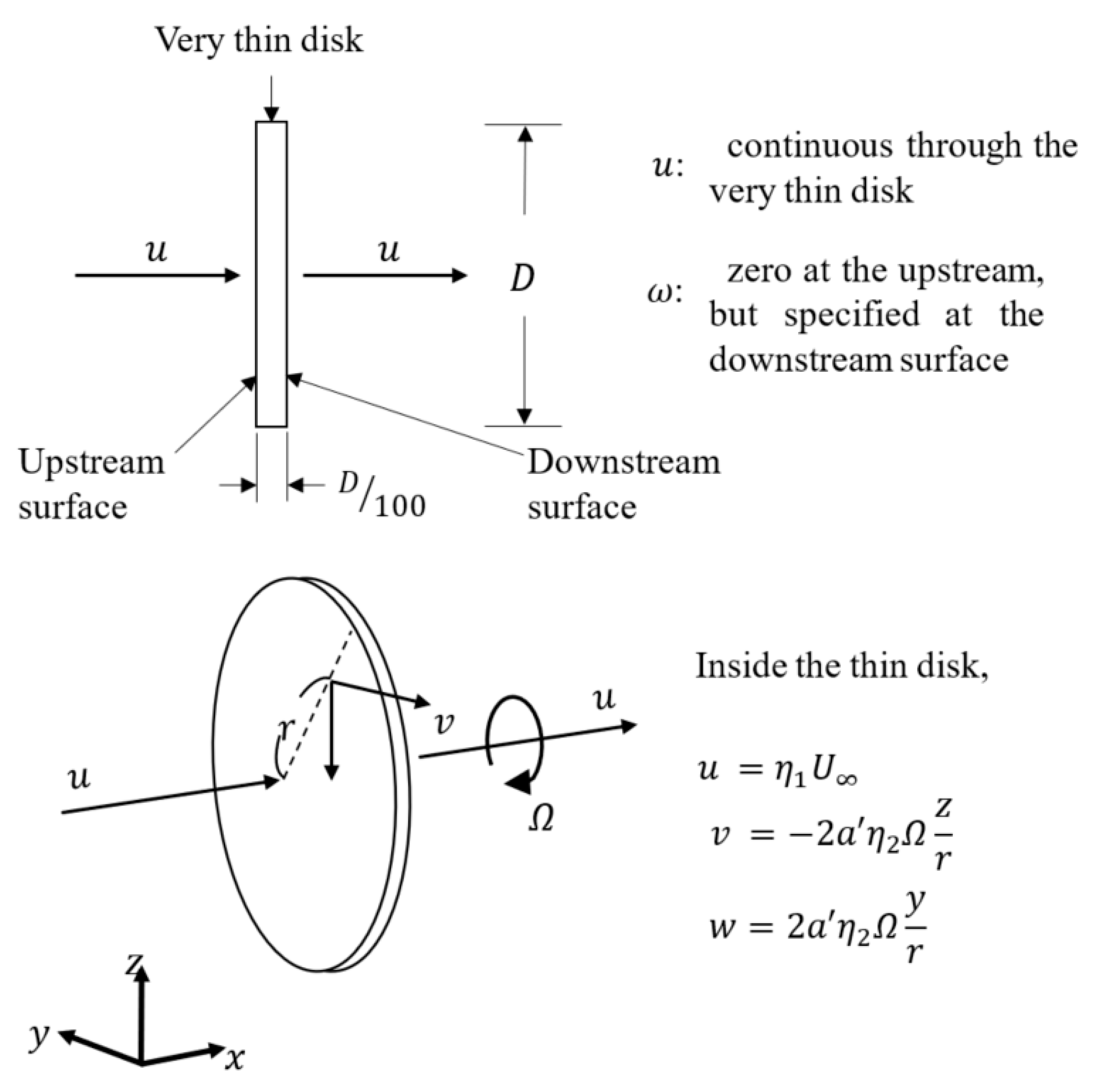
where the velocity ( U ) and the height ( H ) are referenced at the hub of rotor, and the outlet pressure is open to the ambient condition. In the aft surface of the tiny disk area, the velocity components are just forced at the range of actuating disk as shown in Figure 3 where three components of velocity are modeled as:
u = U η 1
v = 2 η 2 a Ω z r
w = 2 η 2 a Ω y r
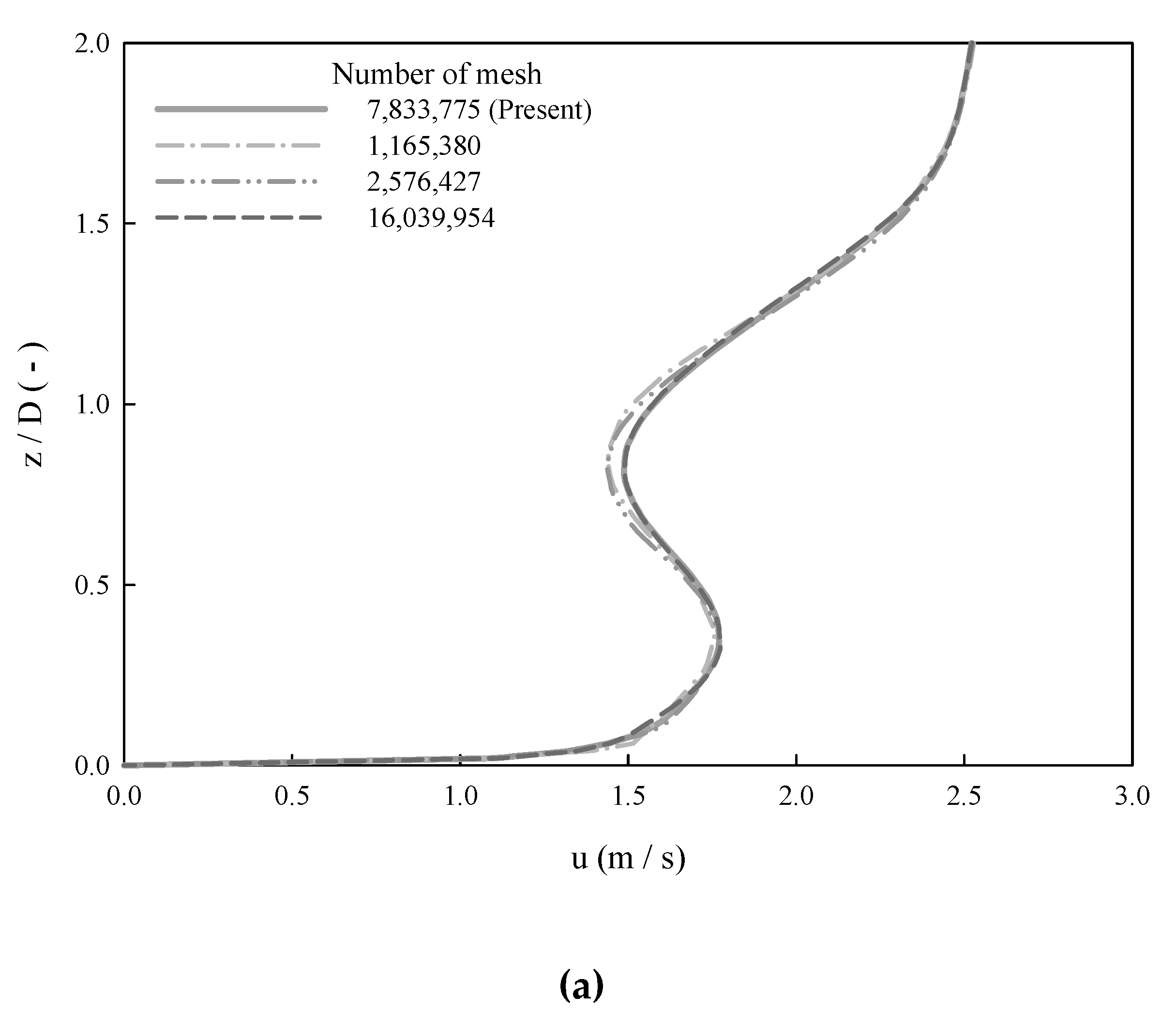
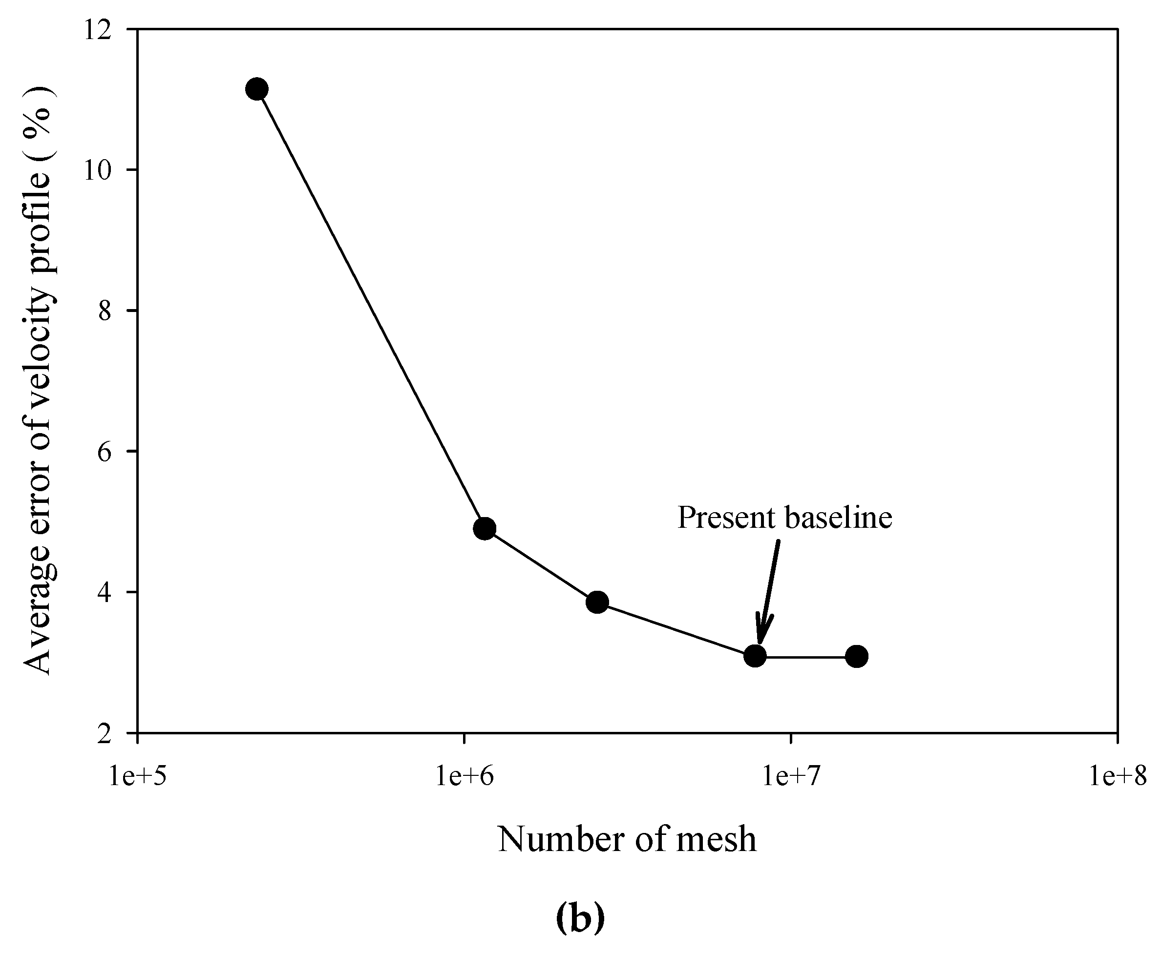
The velocity is specified as an outlet condition of axial component, Equation (14) at the upstream surface of the thin disk, and the rotational components, Equations (15) and (16), are added as an inlet condition with the rotational induction factor a obtained in Equation (12). Since the wake is obviously affected by the turbulence intensity, it is selected to be 5% for wind tunnel tests and 15% for real wind farm simulations in this research. The computational grid is verified in Figure 4a,b. In Figure 4a, the velocity profiles for different scales of meshes are compared with each other, which will also be compared with Figure 5a, and the gird convergence is tested to obtain the present baseline mesh scale for the comparison of average error of velocity profile in Figure 4b.
A commercial code ANSYS-CFX 18.0 (ver.18.0, Ansys Inc., Canonsburg, Pennsylvania, USA) is used with finite-volume discretization, and the k ω SST (shear stress transport) turbulence model is used for every computation, which is chosen to check the strong interaction between the three-dimensional flow at the wake of disk and the turbulent boundary layer at the bottom of computational domain. For the LES (large eddy simulation) computation of counterpart, two types of sub-grid models are used: with the parameter for the effect of turbulent vortex motion and for lift and drag forces induced from the turbine. Actuator disk model (ADM) and actuator line model (ALM) are applied for the load of wind turbine to capture the important characteristics at the wake flow [13].
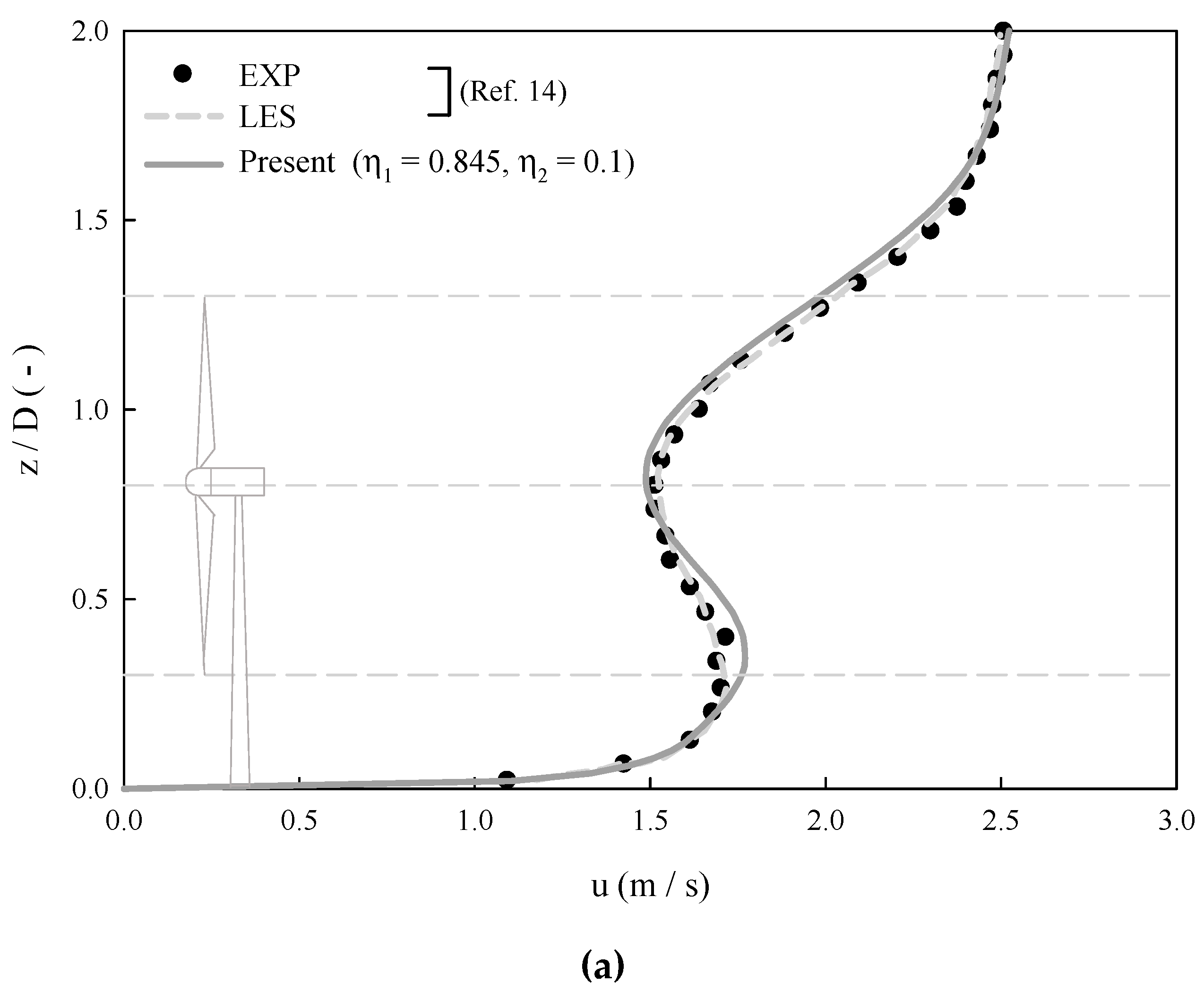
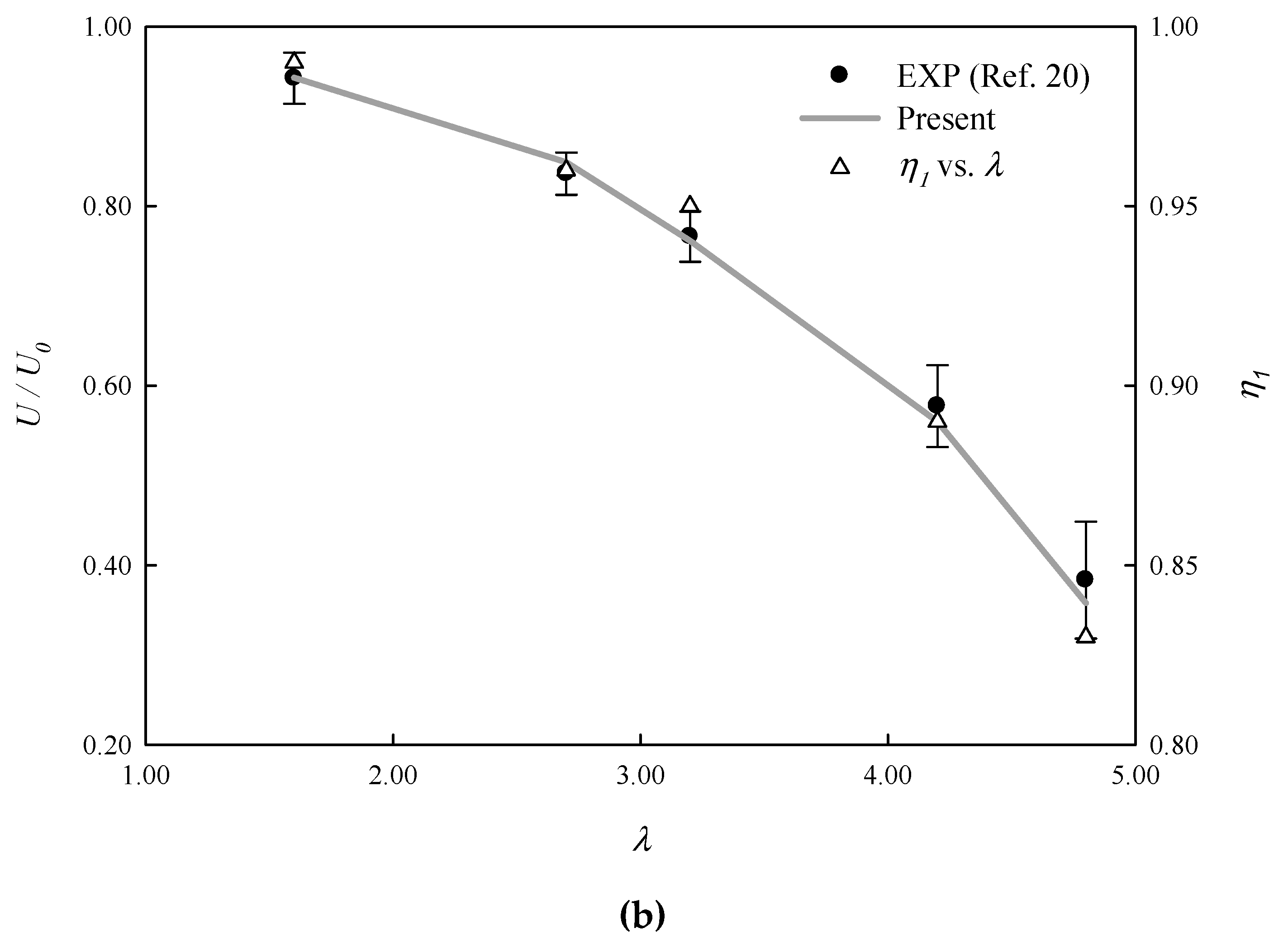
The independent parameters η 1 and η 2 must be found from the empirical data [14], and one of the results is compared in Figure 5a, the velocity profile at the position, x / D = 5 : the mean relative error is 3.1% (or 9.5% maximum) when η 1 = 0.845 , η 2 = 0.1 , and λ = 4 . In the data of Figure 5b, this comparison shows that η 1 decreases as λ increases, or higher power deficit at rapider rotation. However, at the rated value, 6 < λ < 7 , the η 1 seems to approach near the Betz’s limit, η 1 = 2 / 3 at the near field x / D = 1.1 from the disk plane. Although the result of Figure 5 is that of λ = 4 for a slower turbine than the rated one, this method of parameter tuning should be valid because the difference can be aligned from the flow similarity, and the aerodynamic characteristics are not much affected from the rated ones.
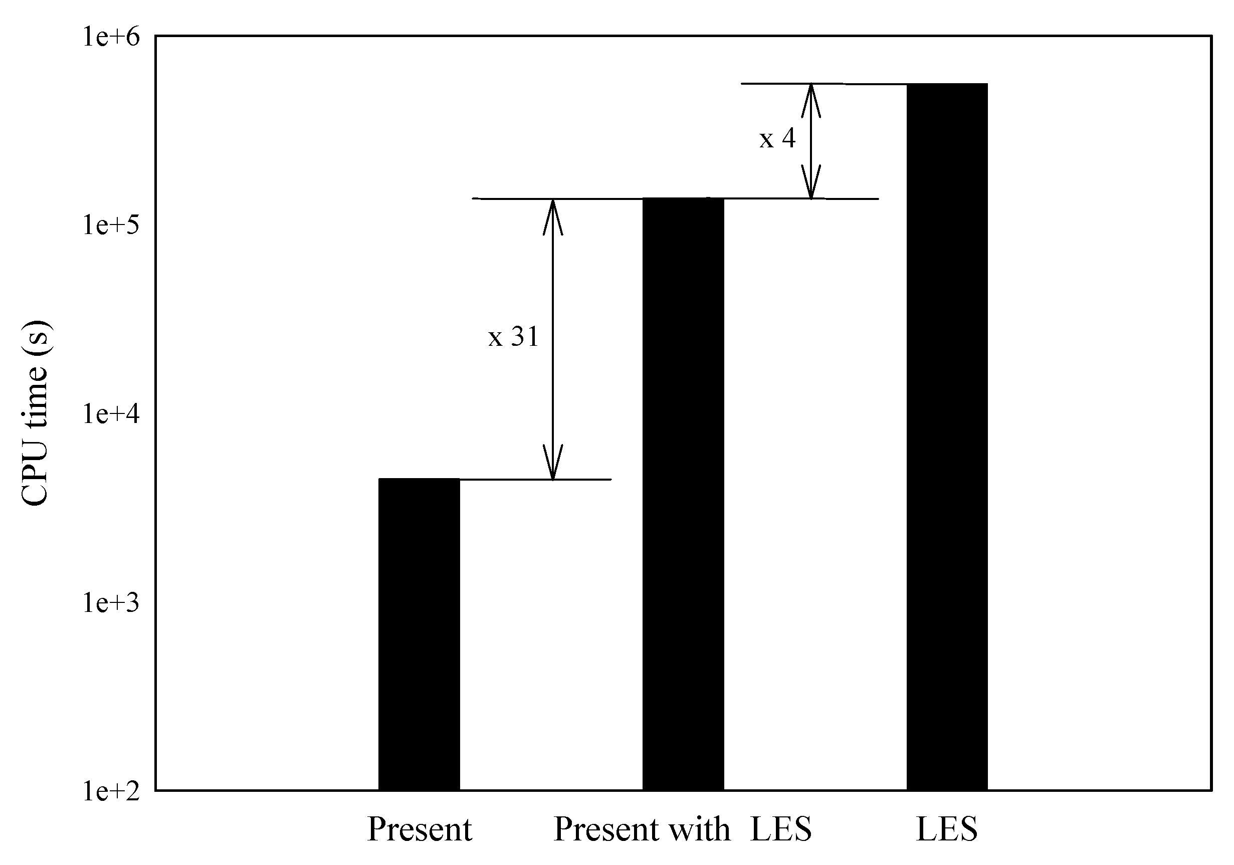
The computational load of CPU time is compared in Figure 6 with RANS computation and LES (large eddy simulation), applying the present disk model boundary conditions and, additionally, we also made a comparison for the full simulation with LES. Using the RANS model, the computational load decreases by 31-times while it is measured as 120-times from the full simulation (without any model) of LES. Therefore, the application of the present disk model remarkably reduces the computation time.

2.3. CFD Model: Multiple Turbines

In Figure 7a, the minimum velocity distribution is plotted along the central axis of rotor, and the present disk model result is compared with Horns Rev1 measurement data [16] in Figure 7b for the inline serial configuration. In Figure 7b, extended eddy viscous wake model [15] and porous disk model [16] are compared in parallel for this case.
The extended eddy viscous wake model is extended from the Gaussian function proposed by Ainslie, which reflects the variation characteristics of eddy viscosity coefficient due to atmospheric condition as well as the experimental function of eddy viscosity. The main procedure to calculate the velocity components, u i , j , in the wake is to solve the system of the following discretized simultaneous equations constructed with Crank-Nicolson (radial direction) and implicit Euler (axial direction) methods:
e M j u i + 1 ,   j 1 + e A j u i + 1 ,   j + e P j u i + 1 ,   j + 1 = r M j u i ,   j 1 + r A j u i ,   j + r P u i ,   j + 1
where the matrix coefficients are defined as Equations (18)–(23):
e M j = v i ,   j 4 Δ r + ε 4 ( Δ r ) r ε 2 ( Δ r ) 2
e A j = u i ,   j Δ x + ε ( Δ r ) 2
e P j = v i ,   j 4 Δ r ε 4 ( Δ r ) r + ε 2 ( Δ r ) 2
r M j = v i ,   j 4 Δ r ε 4 ( Δ r ) r + ε 2 ( Δ r ) 2
r A j = u i ,   j Δ x ε ( Δ r ) 2
r P j = v i ,   j 4 Δ r + ε 4 ( Δ r ) r ε 2 ( Δ r ) 2
where Δ x and Δ r are the axial and radial deviation from the actuator disk, and ε is the eddy viscosity coefficient of the wake.
Since this model is based two-dimensional, the developed velocity profile is shown as a symmetric profile centered on the hub, but the reality is that the velocity near the ground surface is u = 0 . Therefore, the extended viscous wake model [15] adopts the initial wake velocity reflecting the real physics of asymmetry to make a symmetric profile as follows:
U = u * κ ( ln z z 0 ψ W ) D 0 e ( 3.56 r b 2 )
where u * is frictional velocity from the boundary layer; κ is von Karman constant; z is height; the subscript 0 means hub and disk; the offset correction ψ w is given from Businger-Dyer correlations.
The porous disk model shows the decrease of pressure difference before and after the disk plane if the wind speed exceeds 10 m/s that lies before the rated speed, contrast to general porous materials, where the pressure difference is increased when the flow speed increases. The integrated Navier–Stokes equations are expressed in continuity and momentum as follows:
d d t V ρ χ d V + A ρ ( v v g ) n ^ d A = V S u d V
d d t V ρ χ v d V + A ρ v ( v v g ) n ^ d A = A p I n ^ d A + A T n ^ d A + V ( f r + f g + f p + f u ) d V
where χ is the porosity; n ^ is the outward unit normal vector; I is the identity matrix; T is the viscosity stress tensor; f p = P 0 v is the force per volume from the porous region; and P 0 = μ P v + ρ P i | v | / 2 can be decided from P i (porous inertial resistance) and P v (porous viscous resistance) in the equation of equilibrium:
p l = μ P v U + 1 2 P i ρ U 2
where P i = 0.1942 , P v = 0.8350 for less than 10 m/s, and they are specified in Table 1 for more than 10 m/s [16].
The dimensionless parameter where the power output of each turbine is divided by that of the first turbine is computed with the present disk model, and compared with the experimental data, showing a good fit to each other. The extended eddy viscous wake model overall predicted less value while the porous disk model predicted a similar value, but there is a large discord for the second wind turbine. The present model, compared with the extended eddy viscous wake model, simplifies the wake model with no theoretical consideration of turbulence diffusion, and can be applied without specified pressure data as the porous disk model.
The axial induction factor η 1 is listed in Table 2 for each turbine to fit the data, and the efficient of the second turbine decreases (or η 1 increases) much from that of the first turbine. At the later part from the third turbine, the wake developed into a fully mixed turbulent flow, so η 1 is fixed to a constant value, 0.725, independent of the order and position of the rotor.
To see the interactive effect between two disks in the comparison with the Horns Rev1 measurement, as the effect is the most significant in Figure 7b, the boundary condition at the symmetric sides in Figure 8 should be imposed as ‘periodic’ to consider the infinite expansion in the span direction for a wind farm. The height of hub is fixed as 0.7 diameter in all cases. The atmosphere is open on the top of the domain. Two kinds of configurations are possible: staggered and inline.
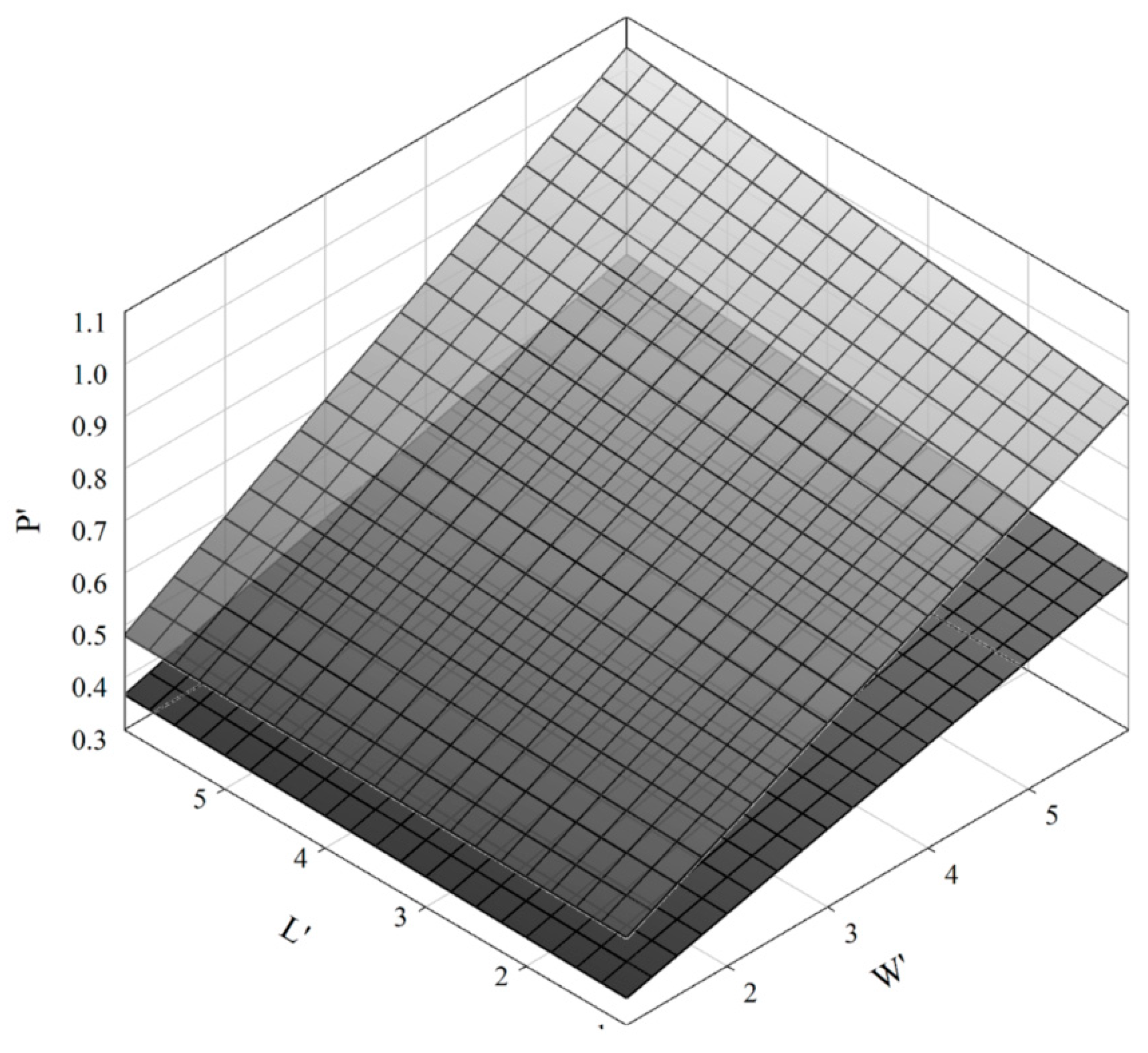
The result in Figure 9 shows a parametric surface of power ratio ( P = P / P 0 ) [23] for the dimensionless length ( L = x / D ) and width ( W = y / D ) where P 0 is obtained from the power from two entirely independent single disks. The correlations are listed as follows:
For the staggered configuration of serial turbines:
P = [ ( W 0.35 ) ( L + 22 ) + 102 ] / 250
For the inline configuration of serial turbines:
P = [ ( 1.3 W + 1.8 ) ( L + 36.6 ) + 235 ] / 1000
The derivatives or sensitivities in Equations (28) and (29) are listed as follows:
P W | s t a g g e r e d = L + 124 250 1 250 L
P L | s t a g g e r e d = W + 102 250 1 250 W
P W | i n l i n e = 1.3 L + 283 1000 1.3 1000 L
P W | i n l i n e = 1.3 W + 237 1000 1.3 1000 W
From Equations (30)–(33), the sensitivity is independent of the directions of configuration regardless of longitudinal ( L ) or lateral ( W ) ones. Comparing staggered and inline cases, the slope of staggered is almost three times in order that of inline. Therefore, the power efficiency in the staggered configuration increases far more than in the inline configuration, which satisfies the general intuition.

3. Conclusive Remarks

A simple numerical model is proposed in this research to investigate the interference effect on the wake of multiple wind turbines. Two parameters of axial and rotational induction are tuned with experimental wind tunnel and LES data, based on the classical momentum theory without introduction of any other additional parameters. This method is so simple, but easily applicable to CFD techniques, also reducing the computational time.
For the measured data in a real wind farm, Horns Rev1 and its comparison with the CFD result, the present model can be shown feasible for the application. From the computational result for two-row configuration of turbines, two correlations are suggested for staggered and inline configuration. If the parameter tuning becomes more precise than now with abundant field data, it is expected to predict an optimal configuration for multiple turbines in the design process of a wind farm. As this model is far faster 100 times than full LES, it should be addressed economical for the simulation of real wind farm at the conceptual level.

Author Contributions

For research articles with several authors, a short paragraph specifying their individual contributions must be provided. The following statements should be used “conceptualization, S.-M.C. and J.-H.L.; methodology, S.-M.C.; software, J.-H.S.; validation, J.-H.S., J.-H.L. and S.-M.C.; formal analysis, J.-H.S.; investigation, J.-H.S.; resources, J.-H.S.; data curation, J.-H.S.; writing—original draft preparation, J.-H.S.; writing—review and editing, S.-M.C.; visualization, J.-H.S.; supervision, S.-M.C.; project administration, J.-H.L.; funding acquisition, S.-M.C.”

Funding

This work is supported the Human Resources Development Program (grant no. 20194010201800) by the Korea Institute of Energy Technology Evaluation and Planning (KETEP) grants and the human resource development for construction equipment R&D business (grant no. N0001292) by Ministry of Trade, Industry, and Energy (MOTIE).

Conflicts of Interest

The authors declare no conflict of interest. The funders had no role in the design of the study; in the collection, analyses, or interpretation of data; in the writing of the manuscript, or in the decision to publish the results.

References

  1. Manwell, J.; McGowan, J.G.; Rogers, A.L. Wind Energy Explained: Theory, Design, and Application, 2nd ed.; John Wiley & Sons: Hoboken, NJ, USA, 2009. [Google Scholar]
  2. Weihing, P.; Meister, K.; Schulz, C.; Lutz, T.; Krämer, E. CFD simulations on interference effects between offshore wind turbines. J. Phys. Conf. Ser. 2015. [Google Scholar] [CrossRef]
  3. Sanderse, B. Aerodynamics of Wind Turbine Wakes: Literature Review; ECN-E-09-016; ECN Wind Energy: Petten, The Netherlands, 2003; pp. 1–46. [Google Scholar]
  4. Vermeer, L.J.; Sørensen, J.N.; Crespo, A. Wind turbine wake aerodynamics. Prog. Aerosp. Sci. 2003, 39, 467–510. [Google Scholar] [CrossRef]
  5. Crespo, A.; Hernandez, J.; Fraga, E.; Andreu, C. Experimental validation of the UPM computer code to calculate wind turbine wakes and comparison with other models. J. Wind. Eng. Ind. Aerodyn. 1998, 27, 77–88. [Google Scholar] [CrossRef]
  6. González-Longatt, F.; Wall, P.; Terzija, V. Wake effect in wind farm performance: Steady-state and dynamic behavior. Renew. Energy 2012, 39, 329–338. [Google Scholar] [CrossRef]
  7. Husien, W.; El-Osta, W.; Dekam, E. Effect of the wake behind wind rotor on optimum energy output of wind farms. Renew. Energy 2013, 49, 128–132. [Google Scholar] [CrossRef]
  8. Bastankhah, M.; Porté-Agel, F. A new analytical model for wind-turbine wakes. Renew. Energy 2014, 70, 116–123. [Google Scholar] [CrossRef]
  9. Carbajo Fuertes, F.; Markfort, C.D.; Porte-Agel, F. Wind turbine wake characterization with nacelle-mounted wind lidars for analytical wake model validation. Remote. Sens. 2018, 10, 668. [Google Scholar] [CrossRef]
  10. Lee, M.; Lee, S.H.; Hur, N. A numerical study on the effect of mountainous terrain and turbine arrangement on the performance of wind power generation. Trans. KSME(B) 2010, 34, 901–906. [Google Scholar] [CrossRef]
  11. Archer, C.L.; Mirzacisefat, S.; Lee, S. Quantifying the sensitivity of wind farm performance to array layout options using large-eddy simulation. Geophys. Res. Lett. 2013, 40, 4963–4970. [Google Scholar] [CrossRef]
  12. Smith, C.M.; Barthelmie, R.J.; Churchfield, M.J.; Moriarty, P.J. Complex wake merging phenomena in large offshore wind farms. In Proceedings of the 20th Symposium on Boundary Layers and Turbulence, Boston, MA, USA, 9–13 July 2012; American Meteorological Society: Boston, MA, USA, 2012. [Google Scholar]
  13. Wu, Y.T.; Porte-Agel, F. Large-eddy simulation of wind-turbine wakes: Evaluation of turbine parametrisations. Bound. Layer. Meteorol. 2011, 138, 345–366. [Google Scholar] [CrossRef]
  14. Conzemius, R.J.; Lu, H.; Chamorro, L.; Wu, Y.T.; Porte-Agel, F. Development and testing of a wind simulator at an operating wind farm. In Proceedings of the AWEA 2010 Wind Power Conference and Exhibition, Dallas, TX, USA, 23–26 May 2010; Windpower, American Wind Energy Association: Washington, DC, USA, 2010. [Google Scholar]
  15. Son, E.K. Numerical Investigation of Wind Farm Characteristics with Rotor-Wake Interaction and Noise Propagation. Ph.D. Thesis, Seoul National University, Gwanak, Seoul, Korea, 2014. [Google Scholar]
  16. Shin, H.K.; Jang, M.S.; Bang, H.J.; Kim, S.H. Wind turbine wake model by porous disk CFD model. J. Wind. Energy 2013, 4, 68–74. [Google Scholar]
  17. Dilip, D.; Porte-Agel, F. Wind turbine wake mitigation through blade pitch offset. Energies 2017, 10, 757. [Google Scholar] [CrossRef]
  18. Ozbay, A. Experimental Investigations on the Wake Interferences of Multiple Wind Turbines. Master’s Thesis, Iowa State University, Ames, IA, USA, 2012. [Google Scholar]
  19. Whale, J.; Helmis, C.G.; Papadopoulos, K.H.; Anderson, C.G.; Skyner, D.J. A study of the near wake structure of a wind turbine comparing measurements from laboratory and full-scale experiments. Solar. Energy 1996, 56, 621–633. [Google Scholar] [CrossRef] [Green Version]
  20. Hasager, C.B.; Vincent, P.; Badger, J.; Badger, M.; di Bella, A.; Peña, A.; Husson, R.; Volker, P.J.H. Using satellite SAR to characterize the wind flow around offshore wind farms. Energies 2015, 8, 5413–5439. [Google Scholar] [CrossRef]
  21. Wan, S.; Cheng, L.; Sheng, X. Effect of yaw error on wind turbine running characteristics based on the equivalent wind speed model. Energies 2015, 8, 6286–6301. [Google Scholar] [CrossRef]
  22. Shin, J.H.; Chang, S.M. Development of a simplified numerical model for the analysis of the wake flow field of a turbine rotor. Wind. Energy J. 2019, 10, 24–30. [Google Scholar]
  23. Shin, J.H.; Chang, S.M.; Jang, M.N.; Lee, Y.J.; Youn, H.J. Quantitative analysis on the decrease of wind energy from the composition effect of the coastal forest for damage prevention—The correlation of dissipation ratio to stand density. J. Korean Soc. Hazard. Mitig. 2015, 15, 361–368. [Google Scholar] [CrossRef]
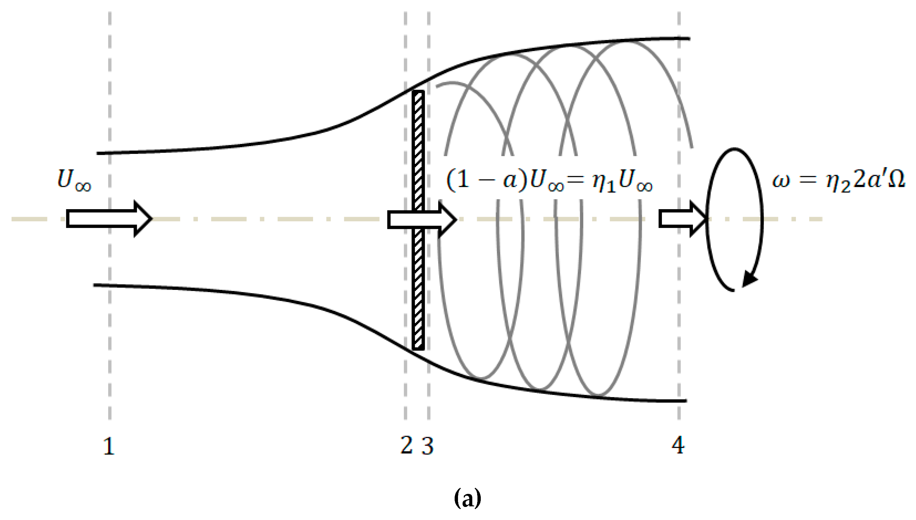
Figure 1. A classical model based on the momentum theory: (a) schematic diagram, (b) axial and rotational induction factors in the BEMT (blade element momentum theory) [1].
Energies 12 04122 g001aEnergies 12 04122 g001b
Figure 2. CFD configuration of model: (a) computational domain; (b) grids system.
Energies 12 04122 g002aEnergies 12 04122 g002b
Figure 3. Disk boundary conditions.
Energies 12 04122 g003
Figure 4. Mesh convergence test: (a) velocity profile; (b) average error of analysis and experiment data [14].
Energies 12 04122 g004aEnergies 12 04122 g004b
Figure 5. The velocity profile at the wake of model: (a) comparison of data [14]; (b) comparison of data [20] ( U / U 0 : centerline velocity ratio at x = 1.1 D from the disk).
Energies 12 04122 g005aEnergies 12 04122 g005b
Figure 6. Comparison of CPU time in seconds.
Energies 12 04122 g006
Figure 7. (a) The velocity along wake direction; (b) Horns Rev1 measurement and the CFD result.
Energies 12 04122 g007aEnergies 12 04122 g007b
Figure 8. Computational domain of the two-low staggered model.
Energies 12 04122 g008
Figure 9. Parametric surface: inline (solid) and staggered (translucent).
Energies 12 04122 g009
Table 1. Rotor inlet and outlet pressure data for wind speed [16].
Wind Speed (m/s) P i P v
11−0.1733.152
12−0.3594.894
13−0.2724.080
14−0.1833.121
15−0.1302.489
16−0.0992.071
17−0.0781.779
Table 2. The axial induction factor η 1 used for each disk in the series of configuration.
Wind Turbine Number1234567
η 1 0.70.750.725