Optimization of Feedforward Neural Networks Using an Improved Flower Pollination Algorithm for Short-Term Wind Speed Prediction

Abstract

It is well known that the inherent instability of wind speed may jeopardize the safety and operation of wind power generation, consequently affecting the power dispatch efficiency in power systems. Therefore, accurate short-term wind speed prediction can provide valuable information to solve the wind power grid connection problem. For this reason, the optimization of feedforward (FF) neural networks using an improved flower pollination algorithm is proposed. First of all, the empirical mode decomposition method is devoted to decompose the wind speed sequence into components of different frequencies for decreasing the volatility of the wind speed sequence. Secondly, a back propagation neural network is integrated with the improved flower pollination algorithm to predict the changing trend of each decomposed component. Finally, the predicted values of each component can get into an overlay combination process and achieve the purpose of accurate prediction of wind speed. Compared with major existing neural network models, the performance tests confirm that the average absolute error using the proposed algorithm can be reduced up to 3.67%.

1. Introduction

Natural energy sources like oil, coal and gas used for power generation are usually environmentally destructive in their harvesting to produce usable energy. They are gone forever when they are used up. Therefore, natural and renewable energy resources from the earth are highly desired. In recent years, wind power has become a new sustainable and renewable alternative to burning fossil fuels, which has a much smaller impact on the environment. With the rapid increase in large-scale wind farms, wind power generation continues to rise in the power industry [1]. For example, renewable energy has generated 72,896 kW power during 2018 in China, with wind power accounting for 25.3% of all this renewable energy capacity [2]. However, the stochasticity and intermittent nature of wind speed may result in an obvious disturbance to the power system and thus affect the power quality. Accordingly, the security and stability of power systems are facing more challenges than before [3]. If the prediction of wind speed can be more accurate, distribution and reserve capacity can be more effectively rationalized through wind turbines. Accordingly, the electricity power spare capacity can be reduced considerably so that smart grids can be achieved [4,5,6,7].

Physical or statistical methods were usually used for wind speed prediction [8,9,10]. In the physical method, for instance, based on the numerical weather prediction model (NWP), a Kalman filter is added for wind speed prediction [11]. However, it requires a large amount of calculations and has a low precision. In [12], the combining of a fuzzy system with a cuckoo search (CS) algorithm was proposed. Compared with the NWP model, this kind of model requires less computation, is faster and more convenient to use. Alternatively, statistical methods, such as time series, support vector machine (SVM) and artificial neural network (ANN), can present a simpler way than the physical methods, but the complexity process of wind speed generation was not fully considered [13]. ANN may suffer from a trapped local optimum and slow convergence speed. Its convergence efficiency may also affect the accuracy of wind speed forecast. On the other hand, a SVM model was reported to improve the function of fluctuating wind speed forecast [14]. Its generalization ability, however, was not enough for the wind speed prediction performance. In [15], the SVM was modified by a new algorithm to reduce the limitations of the model. However, the wavelet basis still has difficulty to achieve an ideal decomposition in the wind speed sequence [16]. In [17], the gray correlation analysis method connected with V-Support Vector Machine (V-SVM) was applied for wind speed prediction. This method has a strong ability for nonlinear fitting, which can realize the wind speed prediction. However, the accuracy is sensitive to the selection of useful fluctuation information from the wind turbine generators. In [18], the LSSVM model predicted the wind speed by integrating the particle swarm optimization (PSO) and gravity search algorithms. A great number of data was demanded to implement the proposed model. In [19], the output and actual situation for wind speed forecast in view of different neural networks were studied and compared. Although the generalization abilities of various models were analyzed, the suitability for different wind farms was not sufficiently unveiled. In [20], the instability of wind speed forecast brought very great difficulty. In this model, a regression model is devoted to predict wind speed, but its forecasting accuracy is still insufficient. In [21], the wind speed sequence is decomposed by the empirical mode decomposition method before prediction. However, the mode aliasing phenomenon may occur and result in an incomplete decomposition.

In the second section of this paper, the principles of feedforward (FF) neural networks and the flower pollination algorithm are introduced. Further, the improved flower pollination algorithm (IFPA) is proposed by adding dynamic inertia weight. Based on IFPA, FF is optimized, and its convergence performance is improved. In Section 3, the ensemble empirical mode decomposition (EEMD) algorithm is presented to deal with the wind speed data. Consequently, the EEMD–IFPA-FF prediction model is established. The forecasting results from EEMD–IFPA–FF, EEMD–FPA–FF and IFPA–FF models are also discussed and compared for details. The conclusions are given in Section 4.

2. Establishment of Forecasting Model

2.1. The Fundamentals of the FF Model

The feedforward (FF) neural network used in this paper is based on a multi-layer feedforward network, which is composed of three layers [22,23]. It can efficiently train the network using a gradient-based optimization algorithm. The network weights and thresholds that connect the input layer and output layer keep updatingiteratively to reduce the error until it reaches the desired task for which it is being trained. The procedures to implement the FF model are shown as follows:

(1)

Initialize all connection weight v and threshold b using small random numbers.

(2)

Determine the structure of the FF model, input training samples and predictive output samples.

(3)

Calculate the outputs of the hidden layer under Equation (1) and the output layer under Equation (2) based on the forward propagation process.

$${\theta }_j^1=f\left({\displaystyle \sum _j^{S_1}{v}_{ji}^1{x}_i+b_j^1}\right),j=1,2,\dots S_1$$

(1)

$${\theta }_k^2=g\left({\displaystyle \sum _j^{S_2}{v}_{kj}^2{x}_j+b_k^2}\right),k=1,2,\dots S_2$$

(2)

where ${\theta }_j^1$ is the output of the hidden layer; $f$ is the transfer function of the hidden layer; $v_{ji}^1$ is the connection weight; $x_i$ is the node of the input layer; $b_j^1$ is the threshold of the hidden layer; $S_1$ is the number of hidden layers; ${\theta }_k^2$ is the output layer; $g$ is the transfer function of the output layer; $v_{kj}^2$ is the connection weight; $x_j$ is the node of the hidden layer; $b_k^2$ is the threshold of the output layer; and $S_2$ is the number of output layers.

(4)

Update weights and thresholds using the back–propagation process, as shown in Equation (3):

$$n(i+1)=n(i)+\beta P(i)$$

(3)

where $n(i+1)$ and $n(i)$ are the weights and thresholds at the $i+1$ and $i$ iteration, respectively; $\beta$ is a learning rate, and $P(i)$ is the negative gradient of the output error at the $i$ iteration, that is, the fastest direction in gradient.

(5)

Repeat Steps (3) and (4) until the mean square error (E) reaches the predefined value:

$$E=\frac{1}{2}{{\displaystyle \sum _k^{S_2}(t_k-{\theta }_k^2)}}^2$$

(4)

where S₂ is the number of output layers; t_k is the target value; and ${\theta }_k^2$ is the output value.

As above, FF may suffer from a weak global search ability, i.e., liable to be trapped into a local minimum. To solve this problem, some algorithms such as extreme learning machines, support vector machines, particle swarms and genetic algorithms are usually used to improve FF [24,25]. In this study, the improved flower pollination algorithm (IFPA) is developed to optimize the FF neural network.

2.2. The Principle of IFPA

The IFPA is developed from the base of the flower pollination algorithm (FPA). Usually, the FPA is performed under the following assumptions: (1) Biological allogamy is a pollinator flying through Levy to achieve a global pollination effect; (2) Self-pollination hypothesis is a local pollination procedure; (3) The reproduction rate of flowers is proportional to the rate of pollination; and (4) The transition between global pollination and local pollination is determined by physical factors, such as distance between flowers or wind speed. This conversion is represented in the algorithm by the conversion probability [26]. The FPA main steps are described below:

(1)

Initializing the parameters, such as the number of flower population N, the transformation probability parameters P and a random number rand ∈ (0,1) in FPA.

(2)

Finding the global optimal solution by comparing the values of the fitness of each solution.

(3)

If the conversion rate is p > rand (a predefined value), the solution is updated, and the transboundary process is implemented in the light of Equation (5):

$$u_i^{t+1}=u_i^t+L\left(g^{*}+u_i^t\right)$$

(5)

where $u_i^{t+1}$ and $u_i^t$ represent the solutions of the ${(t+1)}^{th}$ and ${(t)}^{th}$ generation, separately; $g^{*}$ is the global optimum solution; $L$ is the step length produced by pollen propagator Levyflying; and $L$ obeys the Levy distribution, and its value is substituted into Equation (6):

$$L\sim \frac{\lambda \Gamma \left(\lambda \right)\sin \left(\pi \lambda /2\right)}{\pi s^{1+\lambda }}$$

(6)

where $s>>s_0>0$, $s$ is the step dimension, and $s_0$ is the minimum step dimension; $\Gamma (\lambda )$ is the standard Gamma function, and select $\lambda =1.5$; and the Leavy flight step $L$ is generated under Mantegna’s algorithm [26].

(4)

If the conversion rate is $p\le rand$, the solution is updated, and the transboundary process is implemented according to Equation (7):

$$u_i^{t+1}=u_i^t+\gamma \left(u_j^t+u_q^t\right)$$

(7)

where $\gamma$ is a random number on [0,1]; and $u_j^t$ and $u_q^t$ are pollen of flowers of the same plant species.

(5)

Compute Steps (3) and (4) to get the fitness of the data processing. Judge whether the fitness of the new solution reaches the optimal position. If yes, the fitness and solution is updated. Otherwise, the current fitness and solution remains unchanged.

(6)

If the fitness value of the global optimal is larger than the fitness value of the new solution value, then set a new solution as the global optimal solution.

(7)

Judge whether the end qualification is satisfied. If the conditions are met, the output is certified as the optimal value. Otherwise, return to Step (3).

The principle of FPA indicates that the optimization solution mainly depends on the interaction between pollen individuals, which can be easily trapped into a local minimum. To resolve this problem, the inertia weight $\omega$ is introduced into the pollen position. The new position is updated using Equation (8):

$$u_i^{t+1}=\omega \cdot u_i^t+L\left(g^{*}+u_i^t\right)$$

(8)

At the beginning of the iteration, the larger weight of the previous generation pollen in FPA has a greater impact on the current pollen movement. The attraction between pollen is also smaller. Contrastively, the smaller inertia weight in the later iteration can make the attraction between pollen larger. In this situation, the local search power becomes stronger, while the global search power weakens. To avoid a repeated oscillation near the extreme point from a larger moving step size [26,27,28,29], four inertia weights, i.e., ${\omega }_1$, ${\omega }_2$, ${\omega }_3$ and ${\omega }_4$, are selected to improve FPA, where ${\omega }_1$ is a fixed inertia weight, ${\omega }_2$ is a linear inertia weight, ${\omega }_3$ is an exponential decreasing inertia weight and ${\omega }_4$ is a dynamic inertia weight. Each inertia weight is shown as follows:

$${\omega }_1=0.6$$

(9)

$${\omega }_2={\omega }_{\max }-\frac{{\omega }_{\max }-{\omega }_{\min }}{i_{\max }}\times i$$

(10)

$${\omega }_3={\omega }_{\min }+({\omega }_{\max }-{\omega }_{\min })e^{-{\left(4i/i_{\max }\right)}^2}$$

(11)

$${\omega }_4={\omega }_{\max }-{\left(\raisebox{1ex}{$i$}\!\left/ \!\raisebox{-1ex}{$i_{\max }$}\right.\right)}^3\times \left({\omega }_{\max }-{\omega }_{\min }\right)$$

(12)

where ${\omega }_{\max }$ is the biggest inertia weight; ${\omega }_{\min }$ is the minimum inertia weight; $i$ is the current value of iterations; and i_max is the maximum value of iterations. When the inertial weight varies from 0.9 to 0.4, the optimal searching effect can achieve the best solution [30]. For this reason, select ω_max = 0.9, ω_min = 0.4 and i_max = 200. The variation of four inertial weights vs. iteration number is shown in Figure 1.

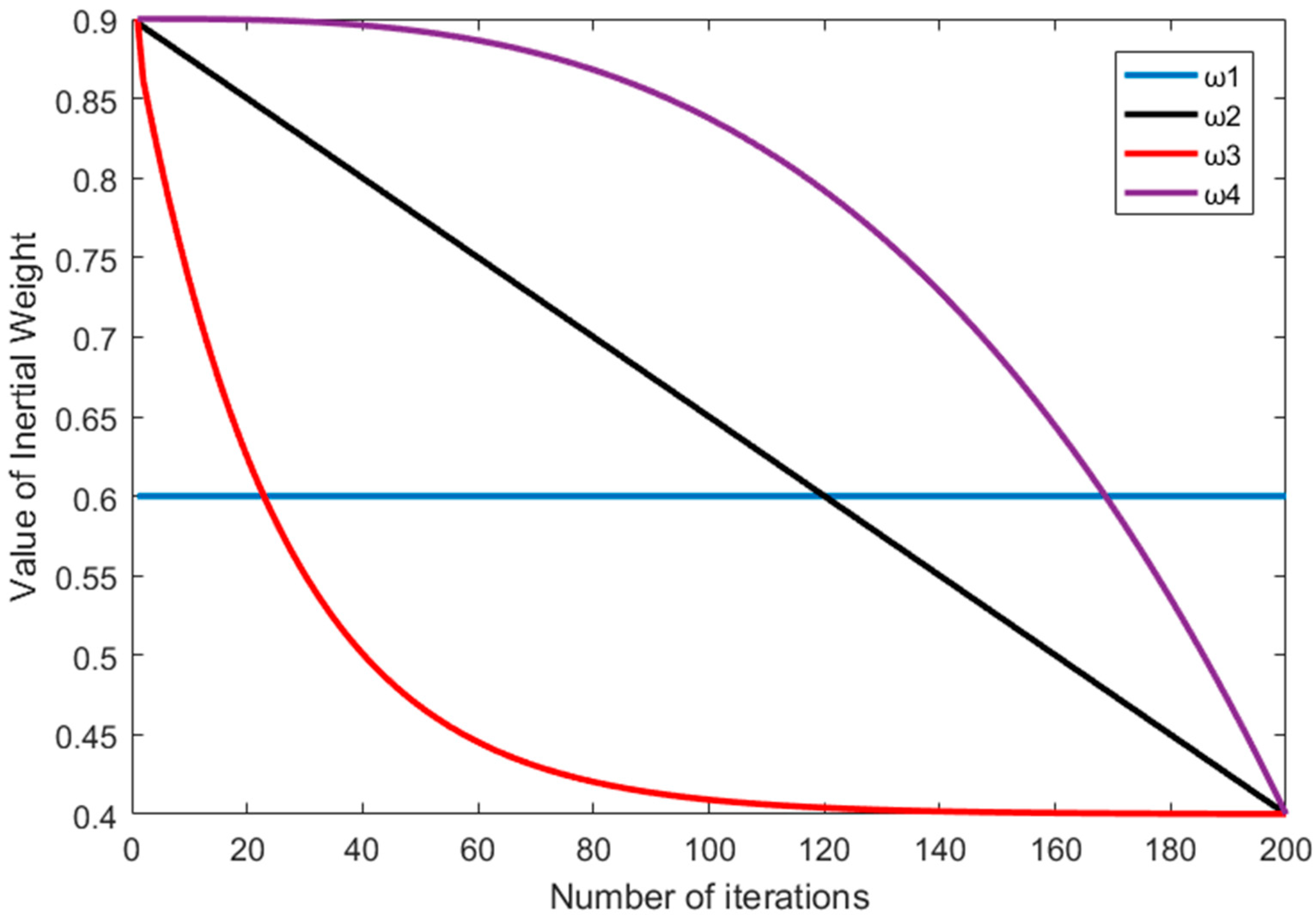
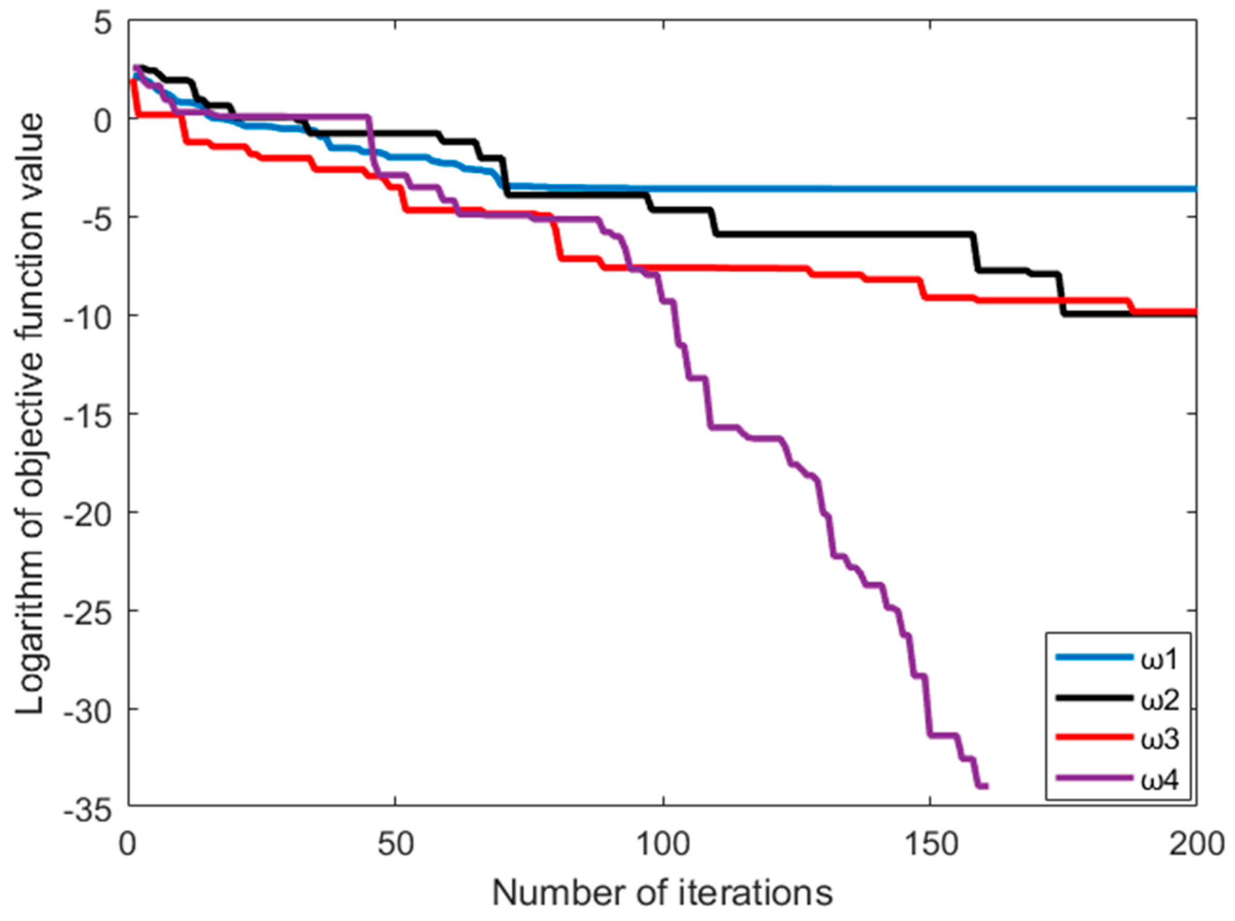
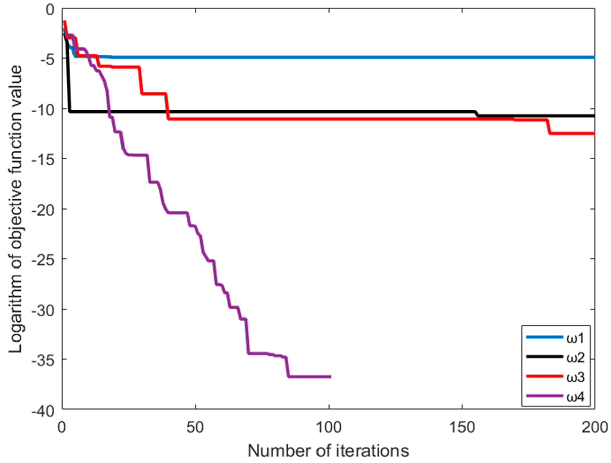
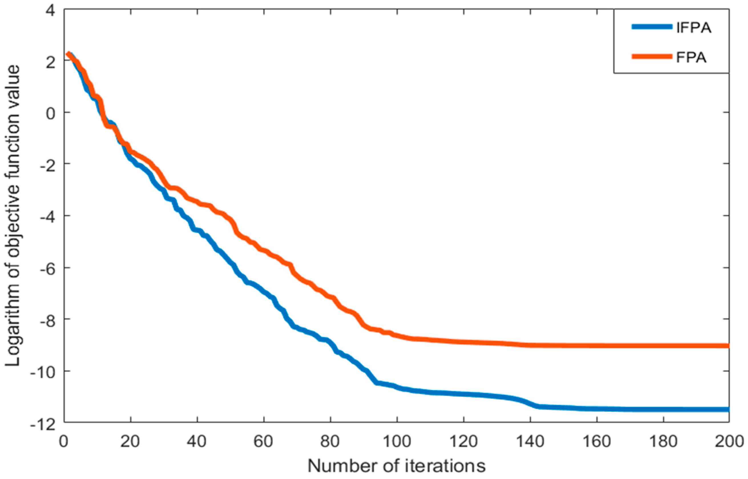
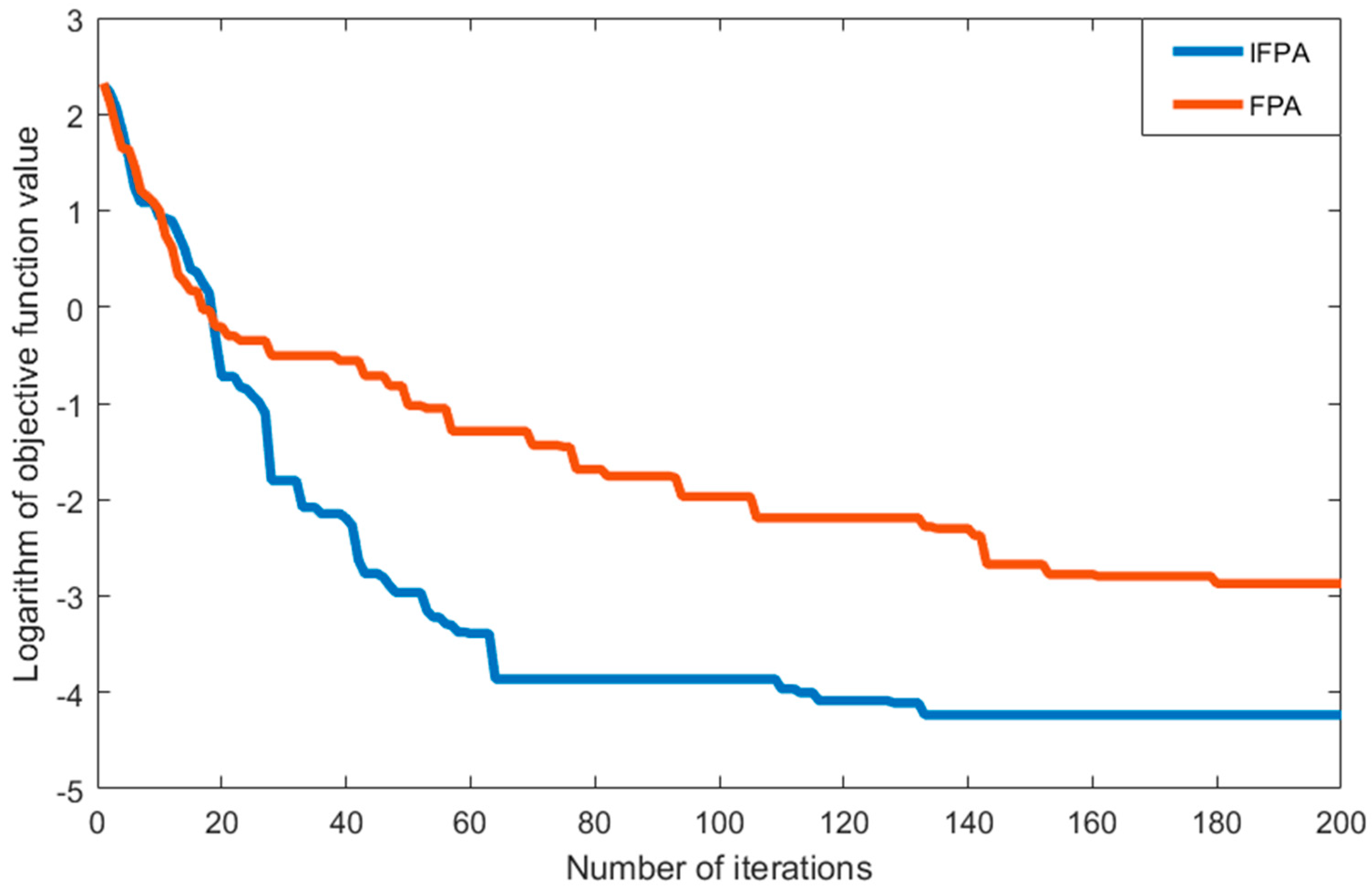
2.3. Convergence of IFPA

In the study, there are four inertia weights, i.e., ${\omega }_1$, ${\omega }_2$, ${\omega }_3$ and ${\omega }_4$, added to IFPA. Rastrigin and Griewank functions are chosen for testing the global optimization performance. The population number, iteration number and conversion probability were set as 20, 200 and 0.8, respectively [31,32]. The parameter settings environment is shown in

Table 1. Parameter settings.

Objective Function	Range	Optimal Value
Rastrigin	x ∈ [−5,5]	0
Griewank	x ∈ [−8,8]	0

. As shown in

Table 2. Test results.

Objective Function	Inertial Weight	Optimal Convergence Value	Worst Convergence Value	Average Convergence Value
Rastrigin	${\omega }_1$	0.0001	0.0265	0.0265
	${\omega }_2$	0.0219	0.0313	0.0271
	${\omega }_3$	2.6130 × 10−10	0.0003	2.6236 × 10−08
	${\omega }_4$	0	0	0
Griewank	${\omega }_1$	0.0742	0.7001	0.0826
	${\omega }_2$	0.0213	0.1301	0.0213
	${\omega }_3$	3.6665 × 10−10	0.2881	2.42 × 10−10
	${\omega }_4$	0	0	0

, the performance results are based on the average of 20 independent tests. It indicates that the optimal solution can be achieved by choosing ${\omega }_4$ in either a Rastrigin or Griewank function.

In Figure 2, the Rastrigin function is taken as the objective function. When the inertia weight is ${\omega }_4$, the optimal value is obtained in the 162${}^{th}$ generation. In Figure 3, the Griewank function is taken as the objective function. When the inertia weight is ${\omega }_4$, the optimal value is obtained in the 101${}^{th}$ generation. Moreover, it proves that ${\omega }_4$ can reach the fastest convergence speed among all parameters.

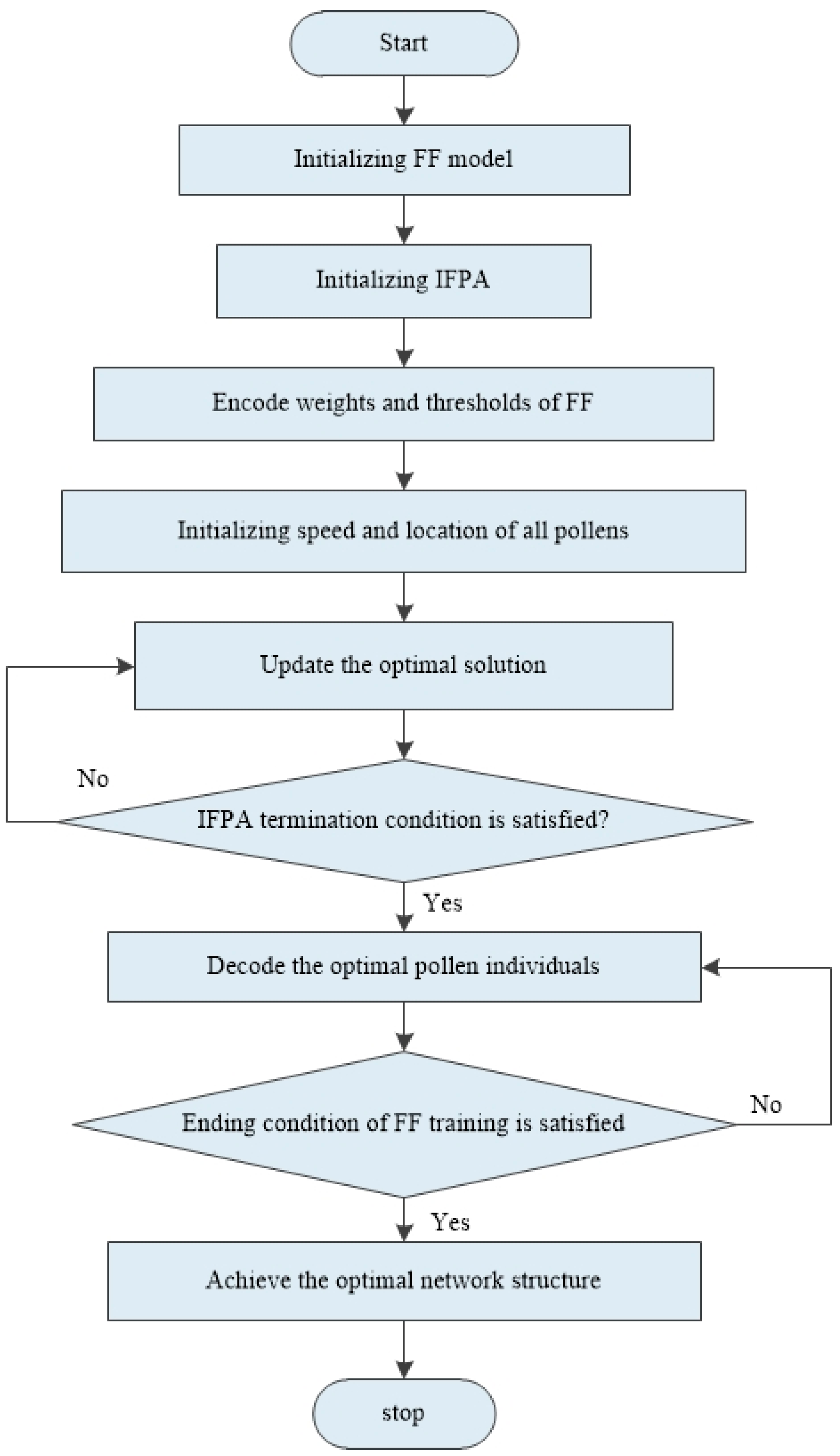
2.4. Optimization of the FF Model Based on IFPA

In this study, the IFPA is integrated with FF neural network to improve the optimization of FF weights and thresholds in the network. The Levy flight characteristics in IFPA are fully utilized for the global searching. Accordingly, the initial weight matrix and bias vector can be found and then given to FF neural network for the training procedure. Figure 4 shows the flow of IFPA–FF, and it is illustrated as follows:

(1)

Initialize FF. Set input layer, hidden layer and output layer, initial network weight v and initial thresholds b.

(2)

Set the population number, the initial value of variation factor and network learning parameters, the maximum number of iterations and training end condition in IFPA algorithm.

(3)

The initial weight v and initial threshold b in FF neural network are encoded into individual pollens u, where each pollen represents the FF neural network structure.

(4)

The speed and position of all pollens are initialized, and the objective function of each pollen is kept computing until the minimum fitness value is reached.

(5)

A random value of rand is generated and compared with the conversion probability p. According to Equations (5) and (7) in FPA, the solution is kept being updated until the global optimal solution is reached.

(6)

If the termination condition of IFPA is met, proceed to the next step. Otherwise, return to Step (5).

(7)

The optimal pollen individual ui is decoded, and the decoded weights vi and bi are used as connection weight v and threshold b for FF.

(8)

If the ending condition of FF training is satisfied, the optimal network structure is thus obtained for further prediction. Otherwise, go back to Step (7).

Schaffer and Ackley are used as objective functions to test the convergence performance in the IFPA and the FPA. The parameter settings environment is shown in

Table 3. Parameter settings.

Objective Function	Range	Optimal Value
Schaffer	x ∈ [−5,5]	0
Ackley	x ∈ [−8,8]	0

. The population number, iteration number and conversion probability were set as 20, 200 and 0.8, which are the same as the parameter settings in the above IFPA. The performance results shown in

Table 4. Test results.

Objective Function	Model	Optimal Convergence Value	Worst Convergence Value	Average Convergence Value
Schaffer	IFPA	3.3621 × 10−79	0.0119	1.0221 × 10−65
	FPA	1.1867 × 10−15	0.0661	0.0001
Ackley	IFPA	2.5426 × 10−74	0.0379	3.7926 × 10−59
	FPA	2.1884 × 10−05	0.0661	0.0661

are based on the average value from 20 independent tests.

The iterative convergence curves using Schaffer and Ackley functions are shown in Figure 5 and Figure 6, respectively. It can be seen that the IFPA model presents the best convergence performance in both of functions.

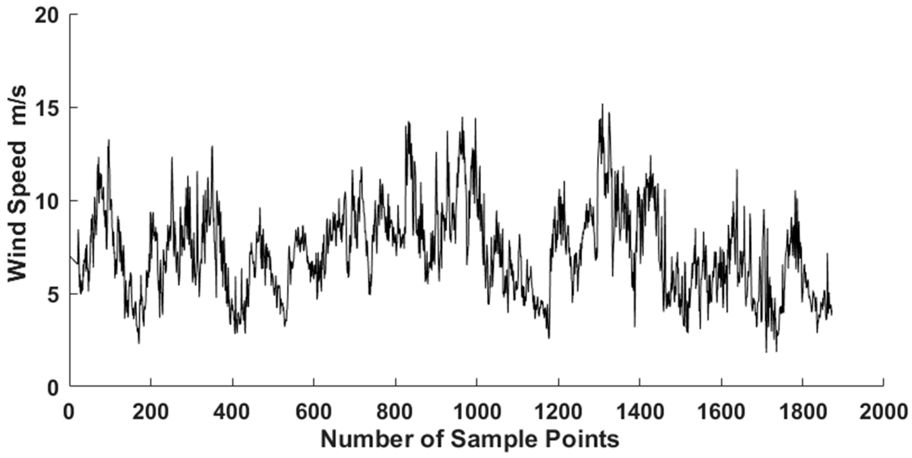
3. Analysis of Wind Speed Forecasting

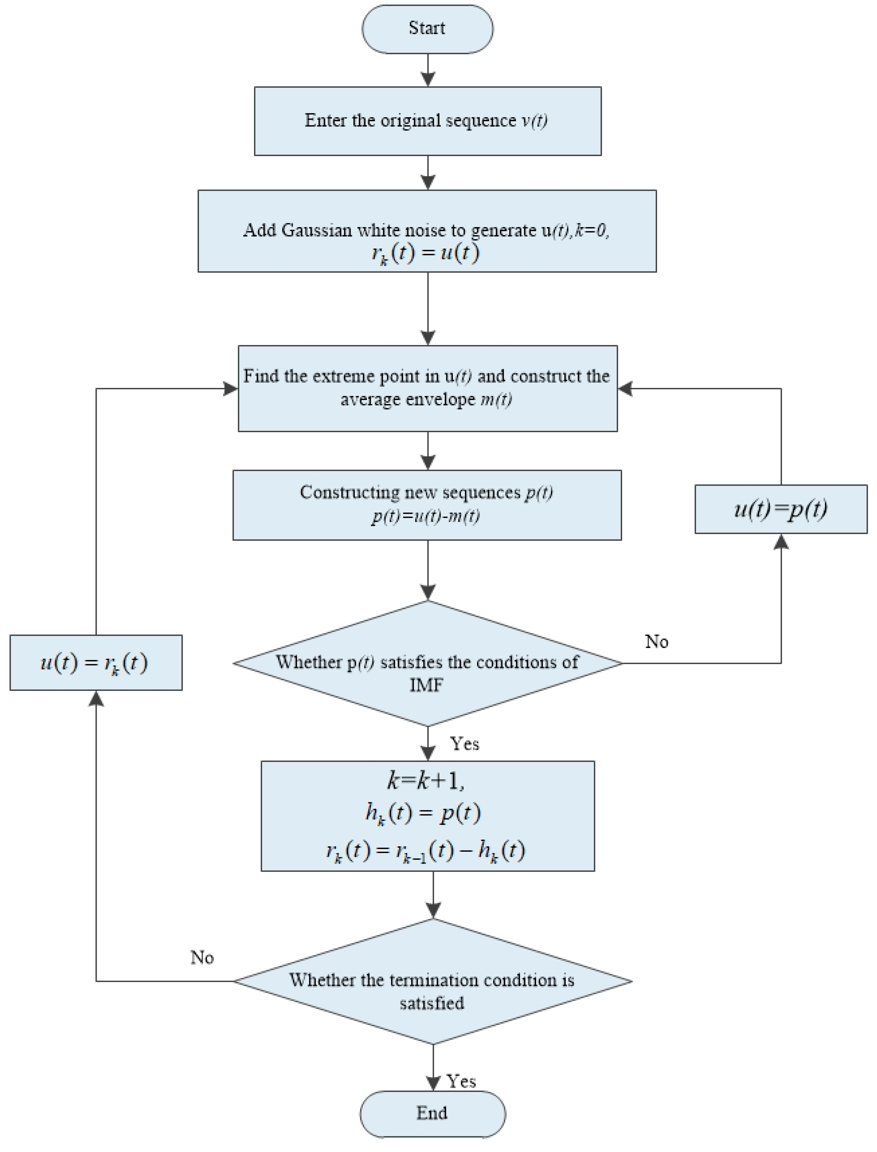
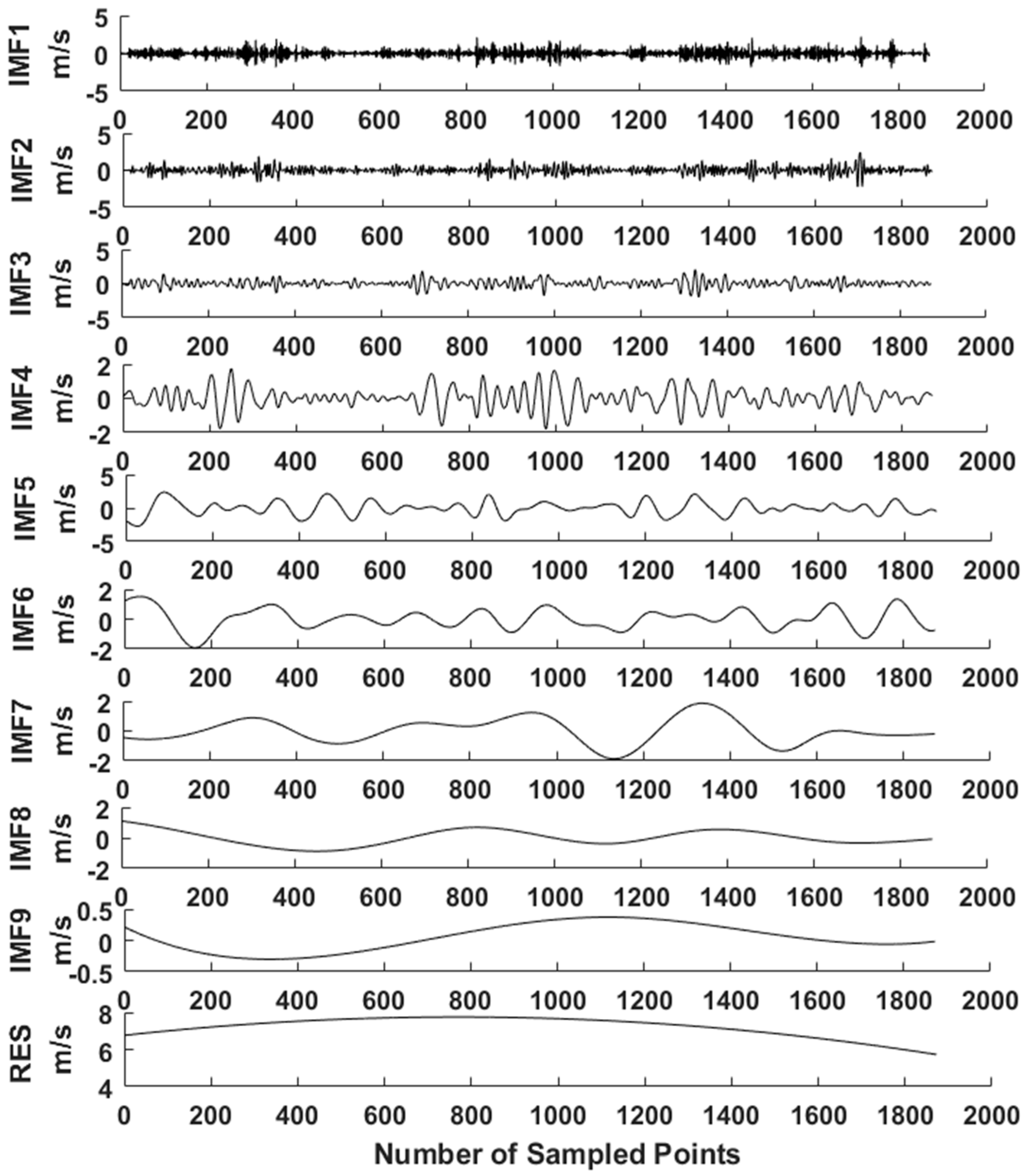
3.1. Preprocessing of Wind Speed Data

The EEMD is an improved EMD model [33]. Based on EMD, a set of Gaussian white noise with normal distribution is added, which effectively improves the aliasing and discontinuity of signals at different scales and avoids the mode aliasing caused by EMD decomposition process [34,35,36]. The flowchart of EEMD is shown in Figure 7, illustrated as follows:

(1)

A normal white Gaussian noise sequence $v(t)$ was added to the original sequence $g(t)$ to generate a new sequence $(u(t)=v(t)+g(t))$.

(2)

Find the maximum and minimum values in $x(t)$ and fit the upper envelope $I_{\max }(t)$ and the lower envelope $I_{\min }(t)$ of $u(t)$.

(3)

Calculate the average envelope $m(t)\left(=\frac{I_{\min }(t)+I_{\max }(t)}{2}\right)$, and subtract it from the noise sequence $u(t)$ to form a new sequence $p(t)(=u(t)-m(t))$.

(4)

Justify if $p(t)$ satisfies the IMF. If yes, the IMF, denoted as $h_1(t)$, is confirmed. Otherwise, repeat Steps (1) and (2) until it is satisfied.

(5)

The $h_1(t)$ is subtracted from the original sequence $u(t)$, and the residual component $r_1(t)(=u(t)-h_1(t))$ is obtained.

(6)

Repeat the same process from the first step until $r_k(t)$, as shown in Equation (13), becomes a monotone function.

(7)

Finally, $u(t)$ is decomposed into k IMFs with different oscillation modes, as shown in Equation (14).

$$\{\begin{array}{c}{r}_2\left(t\right)=r_1\left(t\right)-h_2\left(t\right)\\ r_3\left(t\right)=r_2\left(t\right)-h_3\left(t\right)\\ r_4\left(t\right)=r_3\left(t\right)-h_4\left(t\right)\\ \begin{array}{c}⋮\\ r_k\left(t\right)=r_{k-1}\left(t\right)-h_k\left(t\right)\end{array}\end{array}$$

(13)

$$u(t)={\displaystyle \sum _{i=1}^k{h}_i}(t)+r_k(t)$$

(14)

The data used in this study comes from the Sotavento wind farm in Galicia, Spain, and it is taken from 1 March to 13 March 2018. The wind speed statistics data is shown in

Table 5. Wind speed statistics data.

Maximum (m/s)	Minimum (m/s)	Mean (m/s)	Mode (m/s)	Mid-Value (m/s)	Standard Deviation (m/s)
15.18	2.28	7.47	8.82	7.51	2.59

. Sampling interval of wind speed data was 10 min, as shown in Figure 8.

From Table 5, it is seen that the real wind speed data is highly volatile and unpredictable. Based on the EEMD, it can be decomposed into several relatively stable series under different characteristic scales. The decomposition results are shown in Figure 9.

As shown in Figure 9, the frequency of each component is, in turn, from high to low, and the large fluctuation of high frequency component is the random influence part of wind speed. The low frequency component has the characteristics of a sinusoidal wave and is generally considered as the periodic component of wind speed. The symbol “RES” represents the trend component, indicating the long-term trend of wind speed. There are 10 decomposed sequences (IMF1, IMF2, …, IMF9, RES) input into the IFPA–FF model for training. After the training process is completed, these 10 predicted components are superimposed to obtain the final prediction value for comparison with the real value. The flowchart of the prediction model is shown in Figure 10.

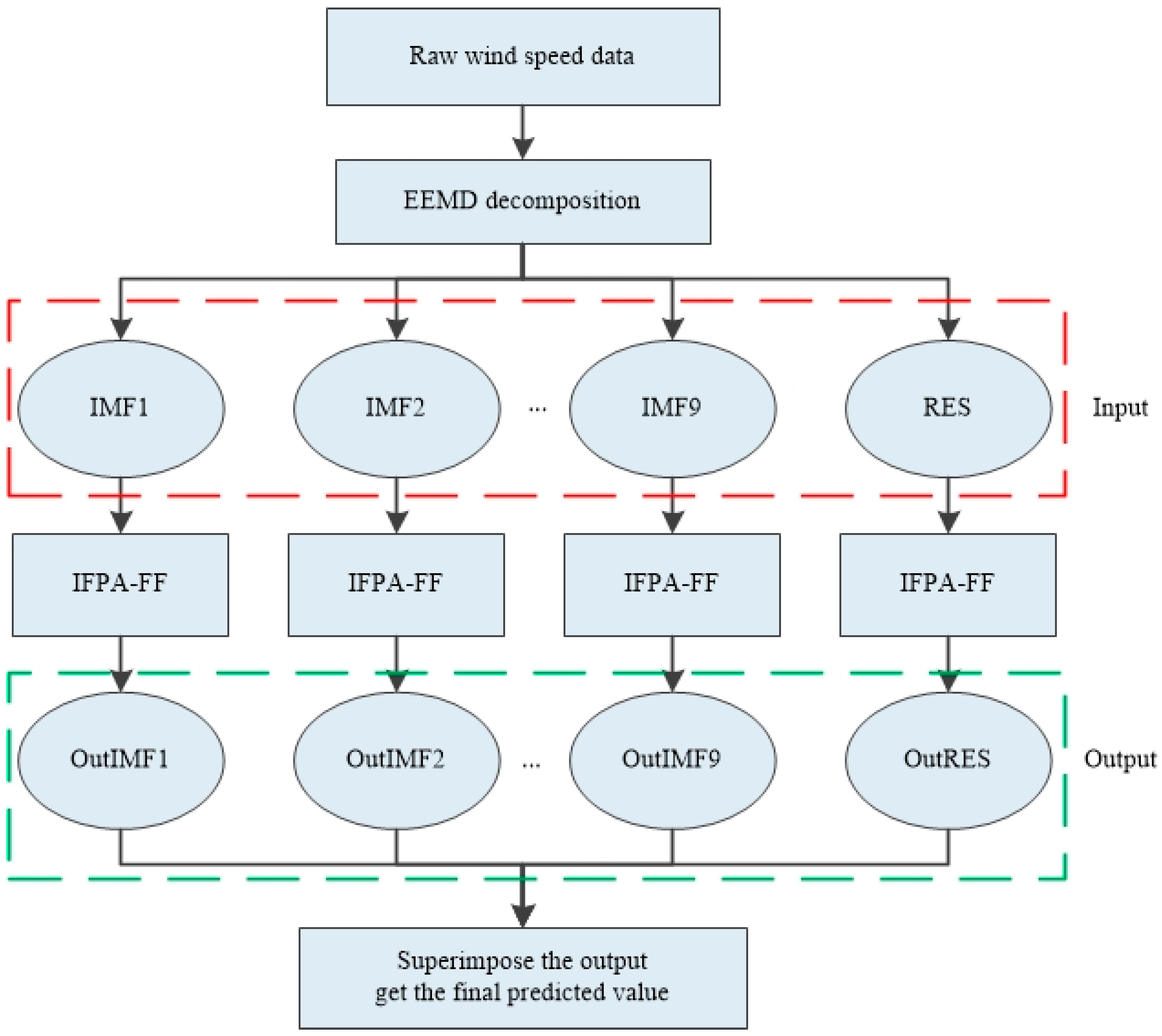
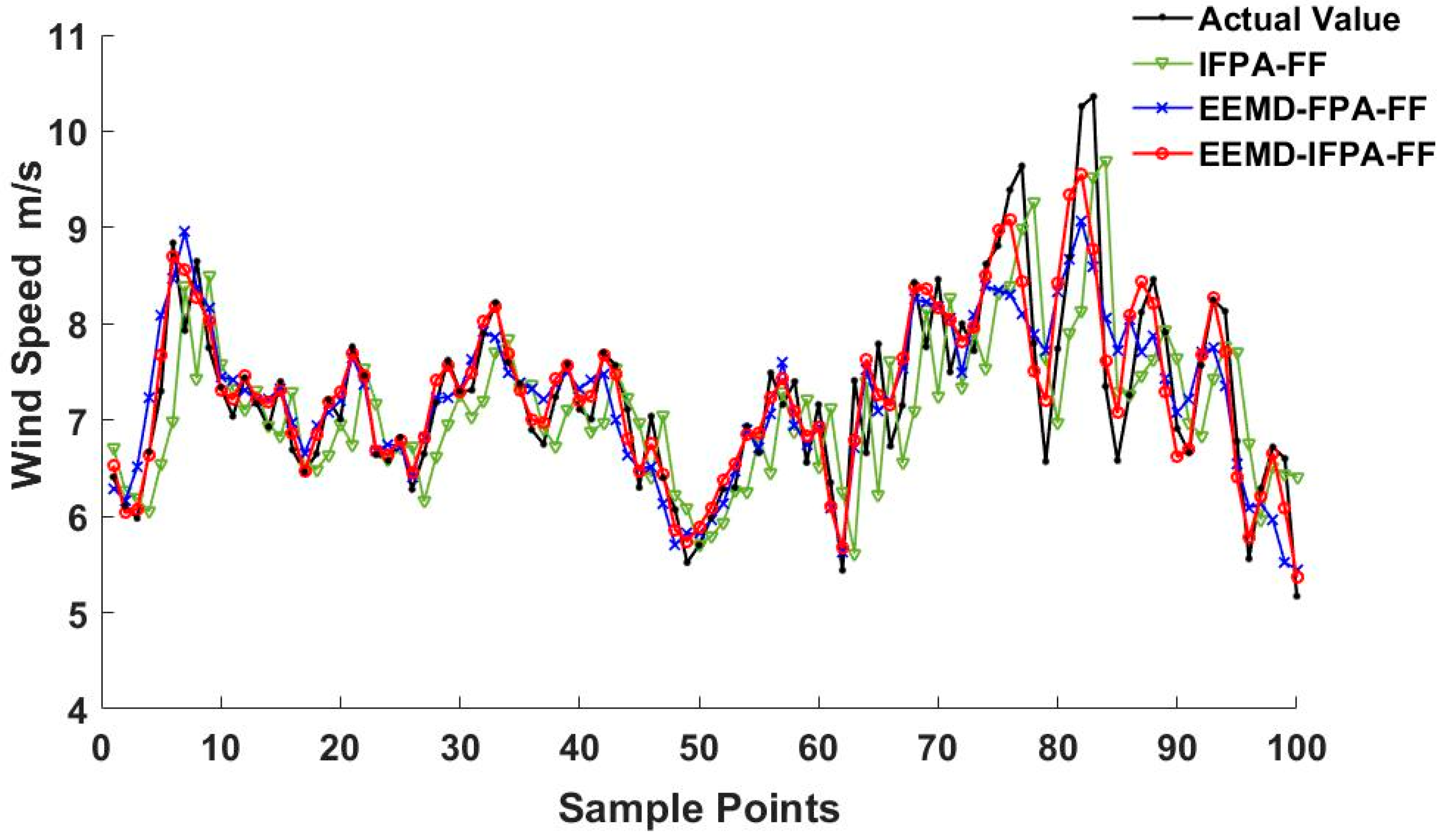
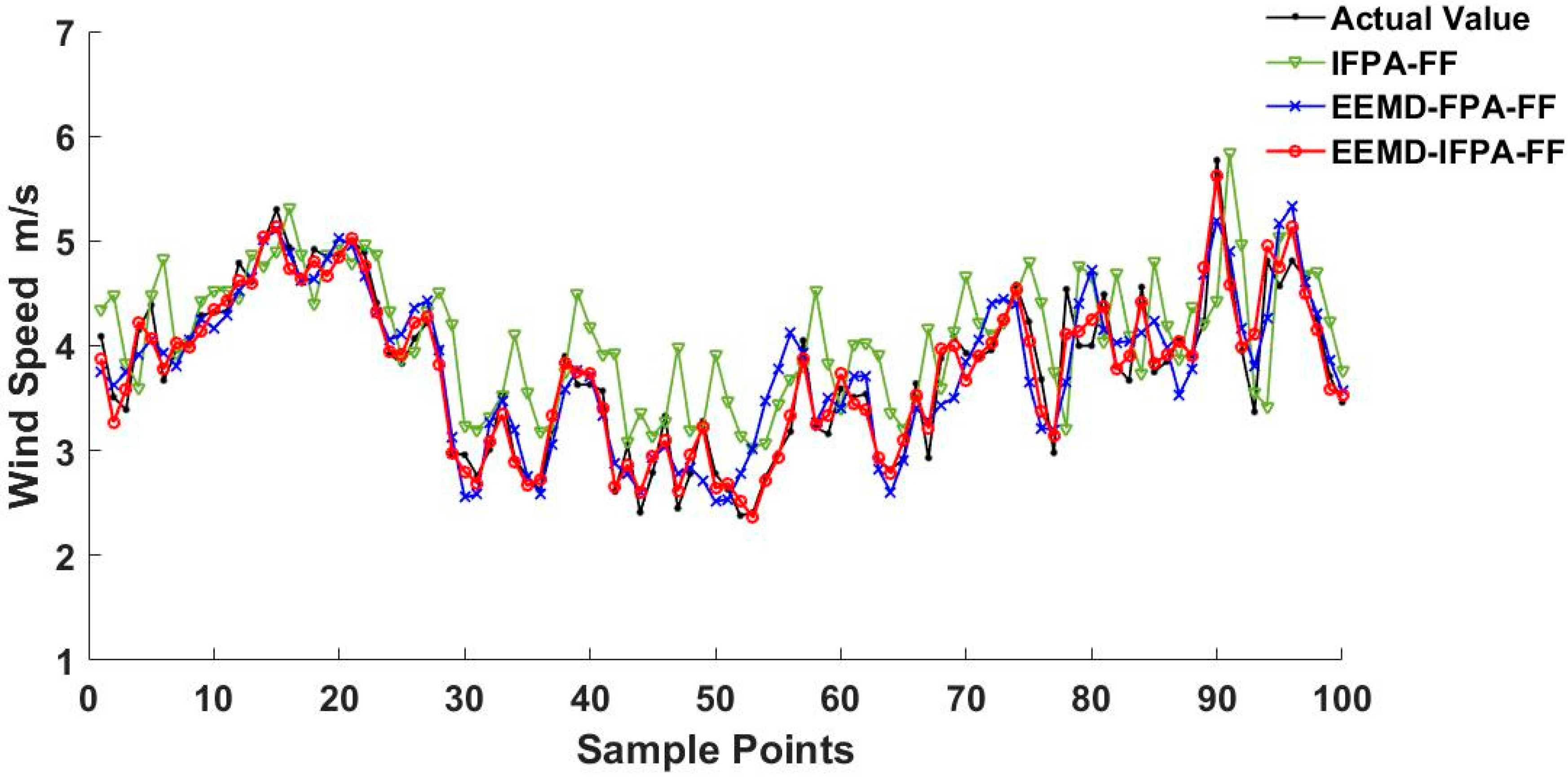
3.2. Wind Speed Forecasting Employed EEMD–IFPA–FF Model

There are three error functions, i.e., MAE, RMSE and MAPE applied to evaluate the effectiveness of the proposed model. Besides, an indicator R_-Squared is employed for calculating the fitness of the model.

$$\mathrm{MAE}=\frac{1}{n}{\displaystyle \sum _{i=1}^n\left|x_i-x_i^{\prime }\right|}$$

(15)

$$\mathrm{RMSE}=\sqrt{\frac{1}{n}{\displaystyle \sum _{i=1}^n{\left(x_i-x_i^{\prime }\right)}^2}}$$

(16)

$$\mathrm{MAPE}=\frac{1}{n}{\displaystyle \sum _{i=1}^n\left|\frac{x_i-x_i^{\prime }}{x_i}\right|}\times 100\%$$

(17)

$$R_{-\mathrm{Squared}}=1-{\frac{{\displaystyle \sum _i^n\left(x_i-x_i^{\prime }\right)}}{{\displaystyle \sum _i^n{\left(x_i-{\overline{x}}_i\right)}^2}}}^2$$

(18)

where n is the forecast sample number; $x_i$ is the value speed at time $i$; $x_i^{\prime }$ is the forecasted value at time $i$; and ${\overline{x}}_i$ is the average of the true value at time $i$.

The initial parameters in this experiment were chosen from References [32,35]. Note that 10 tests were carried out to determine the optimal parameter values in FF and FPA models, concluded in

Table 6. Parameter Settings.

FF
Input Layer Neurons	Hidden Layer Neurons		Output Layer Neurons	Iterations	Target Error		Learning Rate
5	10–5		1	200	0.001		0.01
FPA
Population Number		Dimension		Iterations		Transition Probability
20		10		200		0.8

. The neural network has 15 inputs, 10 neurons in the first hidden layer, 5 neurons in the second hidden layer and one output.

From 1 March to 13 March, a total of 1872 samples were used for model implementation. After EEMD decomposition, 1772 samples of each IMF and RES were trained, and the last 100 samples were used to judge the prediction efficiency. Three models, i.e., EEMD–IFPA–FF, EEMD–FPA–FF and IFPA–FF, were evaluated and compared using the same wind speed data. The comparison between the predicted wind speeds and actual ones on 13 March is shown in Figure 11. It reveals that the predicted curve from EEMD–IFPA–FF model is relatively closer to the actual one than others.

Similarly, the performance test outcomes carried out on 13 February and 13 April can be seen in Figure 12 and Figure 13, respectively. By comparing Figure 11, Figure 12 and Figure 13, the wind speed data in February is relatively stable with less fluctuation and lower amplitude. As a result, each model was more accurate in February than in other months. This implies that the fluctuation of the wind speed and the magnitude is the major factor that may affect the prediction accuracy. The comparison of training samples with existing models is concluded in

Table 7. Error comparison of training samples with existing models.

Time	Model	MAE (m/s)	RMSE (m/s)	MAPE	R-Squared
	EEMD–IFPA–FF	0.1988	0.2097	6.0071%	0.8772
13 February	EEMD–FPA–FF	0.3067	0.4077	7.1021%	0.6912
	IFPA–FF	0.3982	0.5131	9.0831%	0.3144
	EEMD–IFPA–FF	0.2119	0.3019	6.7411%	0.8038
13 March	EEMD–FPA–FF	0.4028	0.5257	9.2269%	0.5981
	IFPA–FF	0.5229	0.6941	11.8581%	0.4719
	EEMD–IFPA–FF	0.3102	0.3931	7.7103%	0.7963
13 April	EEMD–FPA–FF	0.4262	0.5733	9.7835%	0.5492
	IFPA–FF	0.7038	0.8291	13.2210%	0.4045

. The comparison of testing samples with existing models is concluded in

Table 8. Error comparison of testing samples with existing models.

Time	Model	MAE (m/s)	RMSE (m/s)	MAPE	R-Squared
	EEMD–IFPA–FF	0.2287	0.2584	6.2094%	0.8594
13 February	EEMD–FPA–FF	0.3871	0.4440	7.4302%	0.6246
	IFPA–FF	0.4199	0.5670	9.9741%	0.2049
	EEMD–IFPA–FF	0.3079	0.3695	7.2433%	0.7789
13 March	EEMD–FPA–FF	0.4590	0.5728	9.8365%	0.5479
	IFPA–FF	0.5926	0.7802	12.9114%	0.3942
	EEMD–IFPA–FF	0.3699	0.4303	8.3257%	0.7436
13 April	EEMD–FPA–FF	0.5128	0.6817	10.7430%	0.5017
	IFPA–FF	0.7519	0.8924	14.6718%	0.3370

.

Comparing the error results of Table 7 and Table 8, the error of the test set slightly increases compared to the error of the training set. In both training and the test results analysis, the error from the IFPA–FF model performance can reach the smallest value, presenting a certain generalization ability. As shown in Figure 11, Figure 12 and Figure 13, it is found that the wind speed trend prediction using IFPA–FF model has a lag behind the actual speed due to its randomness characteristics. On the other hand, the wind speed series predicted by EEMD–IFPA–FF model and EEMD–FPA–FF model are almost the same as the actual ones without any lag. In Table 8, the maxima errors appeared on 4.13 among three-days collected data. At this day, the MAE, RMSE and MAPE for IFPA–FF model is up to 0.75 m·s⁻¹, 0.89 m·s⁻¹, and 14.67%, respectively. In the EEMD–FPA–FF model, however, the MAE, RMSE and MAPE are down to below 0.51 m·s⁻¹, 0.68 m·s⁻¹ and 10.74%, respectively. In the EEMD–IFPA–FF model, the MAE, RMSE and MAPE are further improved to 0.37 m·s⁻¹, 0.43 m·s⁻¹ and 8.33%, respectively. Compared with the two other existing models, the MAE, RMSE and MAPE are reduced by more than 0.21 m·s⁻¹, 0.30 m·s⁻¹ and 3.67%, respectively. By investigating R_-Squared, it is confirmed that the EEMD–IPFA–FF reaches the highest fitness and achieves a better prediction. In conclusion, it is obvious that the prediction accuracy is considerably improved and relatively stable using the EEMD–IFPA–FF model.

4. Conclusions

In this paper, the proposed EEMD–IFPA–FF prediction model has been well established for an optimization achievement. The FPA is enhanced by incorporating dynamic inertia weights in the IFPA algorithm. Therefore, a faster convergence speed can be achieved. Besides, the FF global search capability is improved to reach a global solution by integrating the IFPA. Moreover, the wind speed data was decomposed using the EEMD method to increase the prediction accuracy. Accordingly, it is obvious that the proposed model provides a better performance than other existing models in both convergence speed and prediction error no matter how small or large the wind speed fluctuates. Apart from the above, the R_-Squared value further verifies the EEMD–IFPA–FF model presents the highest fitness value among existing models.

References

1. William, P.M.; Keith, P.; Gerry, W.; Liu, Y.B.; William, L.M.; Sun, J.Z.; Luca, D.M.; Thomas, H.; David, J.; Sue, E.H. A wind power forecasting system to optimize grid integration. IEEE Trans. Sustain. Energy 2012, 3, 670–682. [Google Scholar]
2. Wang, J.; Song, Y.; Liu, F.; Hou, R. Analysis and application of forecasting models in wind power integration: A review of multi-step-ahead wind speed forecasting models. Renew. Sustain. Energy Rev. 2016, 60, 960–981. [Google Scholar] [CrossRef]
3. Kavousi-Fard, A.; Khosravi, A.; Nahavandi, S. A New Fuzzy-Based Combined Prediction Interval for Wind Power Forecasting. IEEE Transa. Power Syst. 2015, 31, 1–9. [Google Scholar] [CrossRef]
4. Madhiarasan, M.; Deepa, S.N. Comparative analysis on hidden neurons estimation in multi layer perceptron neural networks for wind speed forecasting. Artif. Intell. Rev. 2017, 48, 449–471. [Google Scholar] [CrossRef]
5. Garcia-Ruiz, R.A.; Blanco-Claraco, J.L.; Lopez-Martinez, J.; Callejon-Ferre, A.J. Uncertainty-Aware Calibration of a Hot-Wire Anemometer With Gaussian Process Regression. IEEE Sens. J. 2019, 19, 7515–7524. [Google Scholar] [CrossRef]
6. Sial, A.; Singh, A.; Mahanti, A.; Gong, M. Heuristics-Based Detection of Abnormal Energy Consumption. Smart Grid Innov. Front. Telecommun. 2018, 245, 21–31. [Google Scholar]
7. Sial, A.; Singh, A.; Mahanti, A. Detecting anomalous energy consumption using contextual analysis of smart meter data. Wirel. Netw. J. 2019, 245, 1–18. [Google Scholar] [CrossRef]
8. Wang, Y.; Ma, H.; Wang, D.; Wang, G.; WU, J.; Bian, J.; Liu, J. A new method for wind speed forecasting based on copula theory. Environ. Res. 2018, 160, 365–371. [Google Scholar] [CrossRef]
9. Li, L.L.; Sun, J.; Wang, C.H.; Zhou, Y.T.; Lin, K.P. Enhanced Gaussian Process Mixture Model for Short-Term Electric Load Forecasting. Inf. Sci. 2019, 477, 386–398. [Google Scholar] [CrossRef]
10. Piotrowski, P.; Baczynski, D.; Kopyt, M.; Szafranek, K.; Helt, P.; Gulczynskl, T. Analysis of forecasted meteorological data (NWP) for efficient spatial forecasting of wind power generation. Electr. Power Syst. Res. 2019, 175, 105891. [Google Scholar] [CrossRef]
11. Wang, J.Z.; Wang, S.Q.; Yang, W.D. A novel non-linear combination system for short-term wind speed forecast. Renew. Energy 2019, 143, 1172–1192. [Google Scholar] [CrossRef]
12. Liu, H.; Mi, X.W.; Li, Y.F.; Duan, Z.; Xu, Y. Smart wind speed deep learning based multi-step forecasting model using singular spectrum analysis, convolutional Gated Recurrent Unit network and Support Vector Regression. Renew. Energy 2019, 143, 842–854. [Google Scholar] [CrossRef]
13. Zhao, J.; Guo, Z.; Su, Z.; Zhao, Z.; Xiao, X.; Liu, F. An improved multi-step forecasting model based on WRF ensembles and creative fuzzy systems for wind speed. Appl. Energy 2016, 162, 808–826. [Google Scholar] [CrossRef]
14. Nalcaci, G.; Ozmen, A.; Weber, G.W. Long-term load forecasting: Models based on MARS, ANN and LR methods. Cent. Eur. J. Oper. Res. 2019, 27, 1033–1049. [Google Scholar] [CrossRef]
15. Madhiarasan, M.; Deepa, S.N. A novel criterion to select hidden neuron numbers in improved back propagation networks for wind speed forecasting. Appl. Intell. 2016, 44, 878–893. [Google Scholar] [CrossRef]
16. Wang, J.Z.; Wang, Y.; Jiang, P. The study and application of a novel hybrid forecasting model—A case study of wind speed forecasting in China. Appl. Energy 2015, 143, 472–488. [Google Scholar] [CrossRef]
17. Tascikaraoglu, A.; Sanandaji, B.M.; Poolla, K.; Varaiya, P. Exploiting sparsity of interconnections in spatio-temporal wind speed forecasting using Wavelet Transform. Appl. Energy 2016, 165, 735–747. [Google Scholar] [CrossRef] [Green Version]
18. Alhussein, M.; Harider, S.L.; Aurangzeb, K. Microgrid-Level Energy Management Approach Based on Short-Term Forecasting of Wind Speed and Solar Irradiance. Energies 2019, 12, 1482. [Google Scholar] [CrossRef]
19. Liu, Z.F.; Li, L.L.; Tseng, M.L.; Raymond, R.T.; Kathleen, B.A. Improving the reliability of photovoltaic and wind power storage systems using least squares support vector machine optimized by improved chicken swarm algorithm. Appl. Sci. 2019, 9, 3788. [Google Scholar] [CrossRef]
20. Ding, M.; Zhou, H.; Xie, H. A gated recurrent unit neural networks based wind speed error correction model for short-term wind power forecasting. Neurocomputing 2019, 365, 54–61. [Google Scholar] [CrossRef]
21. Zhao, W.; Wei, Y.M.; Su, Z. One day ahead wind speed forecasting: A resampling-based approach. Appl. Energy 2016, 178, 886–901. [Google Scholar] [CrossRef]
22. Wang, H.Z.; Li, G.Q.; Wang, G.B.; Peng, J.; Jiang, H.; Liu, Y. Deep learning based ensemble approach for probabilistic wind power forecasting. Appl. Energy 2017, 188, 56–70. [Google Scholar] [CrossRef]
23. Ding, Y. A novel decompose-ensemble methodology with AIC-ANN approach for crude oil forecasting. Energy 2018, 154, 328–336. [Google Scholar] [CrossRef]
24. Mohammed, A.; Tomás, M. A review of modularization techniques in artificial neural networks. Artif. Intell. Rev. 2019, 52, 527–561. [Google Scholar] [Green Version]
25. Abdel-Basset, M.; Shawky, L.A. Flower pollination algorithm: A comprehensive review. Artif. Intell. Rev. 2018, 52, 1–25. [Google Scholar] [CrossRef]
26. Li, L.L.; Liu, Z.F.; Tseng, M.L. Enhancing the Lithium-ion battery life predictability using a hybrid method. Appl. Soft Comput. J. 2019, 74, 110–121. [Google Scholar] [CrossRef]
27. Lei, X.; Fang, M.; Wu, F.X.; Chen, L. Improved flower pollination algorithm for identifying essential proteins. BMC Syst. Biol. 2018, 12, 46. [Google Scholar] [CrossRef]
28. Li, L.L.; Zhang, X.B.; Tseng, M.L.; Lim, M.; Han, Y. Sustainable energy saving: A junction temperature numerical calculation method for power insulated gate bipolar transistor module. J. Clean. Prod. 2018, 185, 198–210. [Google Scholar] [CrossRef]
29. Sabeti, M.; Boostani, R.; Davoodi, B. Improved particle swarm optimization to estimate bone age. IET Image Process. 2018, 12, 179–187. [Google Scholar] [CrossRef]
30. Yuan, C.; Wang, J.; Yi, G. Estimation of key parameters in adaptive neuron model according to firing patterns based on improved particle swarm optimization algorithm. Mod. Phys. Lett. B 2017, 31, 1750060. [Google Scholar] [CrossRef]
31. Yang, Y.K.; Jiao, S.J.; Wang, W.F. Cooperative media control parameter optimization of the integrated mixing and paving machine based on the fuzzy cuckoo search algorithm. J. Vis. Commun. Image Represent. 2019, 63, 102591. [Google Scholar] [CrossRef]
32. Li, L.L.; Lv, C.M.; Tseng, M.L.; Song, M.L. Renewable energy utilization method: A novel Insulated Gate Bipolar Transistor switching losses prediction model. J. Clean. Prod. 2018, 176, 852–863. [Google Scholar] [CrossRef]
33. Hu, J.; Wang, J. Wind and solar power probability density prediction via fuzzy information granulation and support vector quantile regression. Int. J. Electr. Power Energy Syst. 2019, 113, 515–527. [Google Scholar]
34. Li, J.H.; Dai, Q. A new dual weights optimization incremental learning algorithm for time series forecasting. Appl. Intell. 2019, 49, 3668–3693. [Google Scholar] [CrossRef]
35. Li, B.; Zhang, L.; Zhang, Q.; Yang, S.M. An EEMD-Based Denoising Method for Seismic Signal of High Arch Dam Combining Wavelet with Singular Spectrum Analysis. Shock Vib. 2019, 2019, 1–9. [Google Scholar] [CrossRef]
36. Tan, Q.F.; Lei, X.H.; Wang, X.; Wang, H.; Wen, X.; Ji, Y.; Kang, A.Q. An adaptive middle and long-term runoff forecast model using EEMD-ANN hybrid approach. J. Hydrol. 2018, 567, 767–780. [Google Scholar] [CrossRef]
Figure 1. Variation of four inertial weights vs. iteration number.
Energies 12 04126 g001
Figure 2. Iterative convergence curve from the Rastrigin function.
Energies 12 04126 g002
Figure 3. Iterative convergence curve from the Griewank function.
Energies 12 04126 g003
Figure 4. Flowchart of the improved flower pollination algorithm–feedforward (IFPA–FF) prediction model.
Energies 12 04126 g004
Figure 5. Iterative convergence curve from the Schaffer function.
Energies 12 04126 g005
Figure 6. Iterative convergence curve from the Ackley function.
Energies 12 04126 g006
Figure 7. Flowchart of ensemble empirical mode decomposition (EEMD) implementation.
Energies 12 04126 g007
Figure 8. Raw data of wind speed.
Energies 12 04126 g008
Figure 9. Data from EEMD decomposition.
Energies 12 04126 g009
Figure 10. Flowchart of the prediction model.
Energies 12 04126 g010
Figure 11. Wind speed prediction on 13 March.
Energies 12 04126 g011
Figure 12. Wind speed prediction on 13 February.
Energies 12 04126 g012
Figure 13. Wind speed prediction on 13 April.
Energies 12 04126 g013