Multi-Objective Optimization for Determining Trade-Off between Output Power and Power Fluctuations in Wind Farm System

Abstract

In this paper, a multi-objective optimization method is proposed to determine trade-off between conflicting operation objectives of wind farm (WF) systems, i.e., maximizing the output power and minimizing the output power fluctuation of the WF system. A detailed analysis of the effects of different objective’s weight values and battery size on the operation of the WF system is also carried out. This helps the WF operator to decide on an optimal operation point for the whole system to increase its profit and improve output power quality. In order to find out the optimal solution, a two-stage optimization is also developed to determine the optimal output power of the entire system as well as the optimal set-points of wind turbine generators (WTGs). In stage 1, the WF operator performs multi-objective optimization to determine the optimal output power of the WF system based on the relevant information from WTGs’ and battery’s controllers. In stage 2, the WF operator performs optimization to determine the optimal set-points of WTGs for minimizing the power deviation and fulfilling the required output power from the previous stage. The minimization of the power deviation for the set-points of WTGs helps the output power of WTGs much smoother and therefore avoids unnecessary internal power fluctuations. Finally, different case studies are also analyzed to show the effectiveness of the proposed method.

1. Introduction

Due to environmental concerns and the shortage of fossil energy sources, conventional thermal electric power generation is gradually being replaced by renewable energy sources (RESs), such as geothermal, solar, wind, biomass, and hydroelectric [1,2]. Among these RESs, wind energy has gained great attention from researchers and industry. By the end of 2017, the global installed capacity has reached 539 GW and this capacity might be reached 840 GW by 2022 [3]. The dramatic growth of wind power in the power system has resulted in the installation of hundreds of wind turbine generators (WTGs) in large geographic areas. The individual operation of each WTG may cause various difficulties for the transmission system operators. Therefore, all WTGs are grouped into a wind farm (WF) system and usually managed by a centralized energy management system, e.g., a WF operator [4,5,6].

The main purpose of the WF operator is to manage the operation of the entire WF system and determine the optimal set-points of WTGs to achieve different operation objectives. A common operation objective in the WF system is to maximize the output power of the entire system. Several studies have suggested different approaches to increase the output power and service reliability of the WF system, such as pitch misalignment detection [7], identification of defective anemometers [8], estimation of wind energy production considering varying air density [9], optimization of the position of WTGs in the WF system [10,11,12], optimization of the operation of WTGs to reduce power loss [13,14], or reduction of wake loss in WF systems [15,16]. The authors in [11] have proposed a new WF layout optimization model for maximizing the equivalent power of a WF system using particle swarm optimization algorithm. The authors in [12] have presented a random search algorithm based on continuous formulation to solve the WF layout optimization problem for providing higher power generation. The authors in [13] have proposed an optimal reactive power dispatch strategy to minimize the total electrical losses of a WF system, including losses inside WTGs, transformers, and losses in the transmission cables. The authors in [15] have presented a distributed approach to solve a WF power maximization problem considering the wake interaction among WTGs using a distributed particle swarm optimization algorithm. The authors in [16] have presented a new methodology for optimizing the wake effect performance by controlling the pitch angle and the tip speed ratio of each WTGs. This minimizes the overall wake effect between WTGs and, therefore, maximizes the power produced by the WF system. The impact of turbulence intensity due to wind turbine wakes in WF system has also been presented in [17] to reduce the power losses and, therefore, increase the output of WF.

The maximization of injected power into the power system can increase the WF’s profits by selling power. However, with the high penetration of wind energy, many large-scale WF systems have recently been developed with output power up to gigawatts (GW) [18,19]. The operation of such WF systems at maximum power point checking (MPPT) can lead to high fluctuations in output power and affect power quality, or even threaten the stability and security of the whole power system [20,21]. Therefore, many studies have proposed different methods to reduce the output power fluctuations of the WF system [22,23,24,25,26]. The authors in [22] have proposed a series of robustness metrics to quantify the ability of WF to produce power with high mean value and low variability under changing wind. This helps to design WFs for producing power with high mean value and low variability. The authors in [23] have presented a novel strategy for minimizing the output power fluctuation from a WF by adjusting the set-points of some WTGs. A battery energy storage system (BESS) has also been used to support the operation of the WF system. The authors in [24] have introduced a method to determine the power dispatch capability of a wind-battery hybrid power system with minimal battery capacity. With the integration of a BESS into the wind power system, the wind power variation can be mitigated to dispatch a constant power to the power grid. The authors in [25] have presented an adaptive control scheme of the superconducting magnetic energy storage units for smoothing the output power of a WF system. The authors in [26] have developed a supervisory control unit to manage a stored energy in a small capacity flywheel energy storage system to reduce the output power fluctuations of a WF system. Using energy storage systems in WF systems not only increases the output power but also reduces the power fluctuations from WF systems. However, the investment costs of large BESSs is still very high. Several studies have suggested different methods to optimize the sizing of BESSs [27]. To reduce output power fluctuation of WF, several studies have also been proposed for filtering the grid harmonics due to the high-voltage direct-current line in WF [28,29].

Based on the above literature review, it can be concluded that most existing methods for the operation of the WF system have only focused on a single operation objective, i.e., maximizing the output power [11,12,13,14,15,16] or minimizing the output power fluctuation [22,23,24,25,26]. However, many WF systems wish to generate maximum output power and preserve a low power fluctuation at the same time. It can be seen that the two operations’ objectives are conflicting. For example, if the WF operators always operate the WFs system at MPPT for maximizing their output power, it could result in high output power fluctuations, especially under high variation of wind energy. Conversely, minimizing the output power fluctuations also results in a decrease in the output power of the WF system [30]. Therefore, the methods introduced in [11,12,13,14,15,16] and [22,23,24,25,26] are not suitable for the operation of WF systems with multi-objective functions. Due to the lack of detailed studies for the operation of WF with the multi-objective function, the WF operators face many diverse hurdles in determining the optimal operation point for these such systems. To help the WF operator optimally operate a WF system that has different operation objectives, it is necessary to study in detail the trade-off between such different operation objectives.

Therefore, a multi-objective optimization method is proposed in this paper for determining a trade-off between maximizing the output power and minimizing the output power fluctuation. The weights of the objective functions in multi-objective optimization have large effect on the operation of the WF system. Therefore, the effect of different weight values on the operation of the WF system is analyzed in detail in this study. Moreover, several WF systems are recently equipped with BESS to improve the performance of the whole system [23,24,25,26]. The effect of BESS size on the operation of the WF system is also presented in detail. Based on these analyses, the WF operator can decide a suitable size of BESS using in this WF system and an optimal operation point for the whole system. In order to find out the optimal solution, a two-stage optimization is developed to determine the optimal output power of the WF system and the optimal set-points of WTGs. In stage 1, the multi-objective optimization is solved to determine the optimal output power of the WF system based on relevant information from local controllers. In stage 2, the optimal operation of WTGs is determined to minimize the power deviation for the set-points of WTGs and fulfill the required power for the WF system from stage 1. The use of the proposed method helps the WF system to balance its profit and output power quality. Furthermore, minimizing the power deviation for the set-points of WTGs can significantly reduce internal power fluctuations in the WF system. Finally, many different scenarios are also presented to evaluate the effectiveness of the proposed method. The major contributions of this study are summarized as follows:

• A multi-objective optimization model is proposed for trade-off between conflicting operation objectives, i.e., maximizing the output power and minimizing power fluctuation from WF. This helps the WF operator to easily determine the optimal operation points for the entire system.
• A detailed analyses considering the different weights for operation objectives and different size of BESS are carried out. Based on these analyses, the WF operator can determine the optimal weights between two operation objectives as well as the optimal BESS size to improve the operation of the WF system.
• The proposed optimization model in the second stage aims to minimize the power deviation for the set-points of WTGs. Minimization of power deviation helps the output power of WTGs be smoother and, therefore, avoid unnecessary fluctuations within the WF system.

The remainder of this paper is structured as follows. Section 2 describes the WF system configuration. Section 3 presents a common problem in the operation of WF system. Section 4 presents the proposed operation strategy for the WF system. Section 5 presents a detailed MILP-based mathematical model for the proposed method. Section 6 discusses the numerical results in different case studies. Section 7 describes the scope for future studies, and Section 8 provides a summary of this study.

2. WF System Configuration

Figure 1 shows a typical WF system with several clusters of WTGs and WTGs in a cluster are connected in series. The output power of the entire WF system is determined by the total power generation from all WTGs. The operation of the entire WF system is usually managed by a centralized energy management system, i.e., a WF operator. The main purpose of the WF operator is to determine the optimal output power from the WF system as well as to determine the optimal set-points of WTGs. Firstly, based on measurement information, such as wind speed, wind direction, and so on, the amount of available generation power from each WTG is determined by its local controller. Then, information of available power is given to the WF operator by WTG’s controller via a communication network. Based on the receiving information, the WF operator determines the maximum output power that can be generated from the WF system and performs optimization to find out the optimal amount of output power. Finally, the WF operator optimally adjusts the set-points of WTGs within the minimum operation point to maximum operation point to achieve the required amount of output power.

3. Problem in Operation of WF System

In this section, a major problem in the operation of WF systems is presented. It can be observed that the operation of WTGs at MPPT can increase the output power for the WF system. This helps the WF operators increase their profit by selling power to the power system. This can be acceptable for the operation of small WF systems due to the small output power and the output power fluctuation does not affect to the power system. However, in large WF systems, if the WF operators always want to operate WFs at MPPT for maximizing their output power, it could result in high output power fluctuations, especially under high variation of wind energy [30]. This results in a significant decrease in power quality from the WF system. These WF operators sometimes face high penalties from the power system.

It can be observed from Figure 2 that the maximum output power of the WF system can cause large power fluctuations in the WF system. On the other hand, if the output power is slightly reduced in peak output intervals (e.g., wind energy curtailment, or charging for BESS), the output power fluctuations from the WF system can be significantly reduced. In some periods of time, the output power is low (e.g., t2 and t4) and will be compensated by discharging power from BESS. Moreover, large WF systems also often have different operation objectives. With different objectives, the WF operators will decide different operation points for each WTGs. However, the operation of the WF system aims to achieve an operation objective, which may conflict with other operation objectives. Therefore, determining trade-off between different operation objectives plays an important role in the operation of the WF system. In the following sections, a detailed model for multi-objective optimization will be presented. In addition, the effects of various parameters on the operation of the WF system are also analyzed.

4. Operation Strategy for WF System

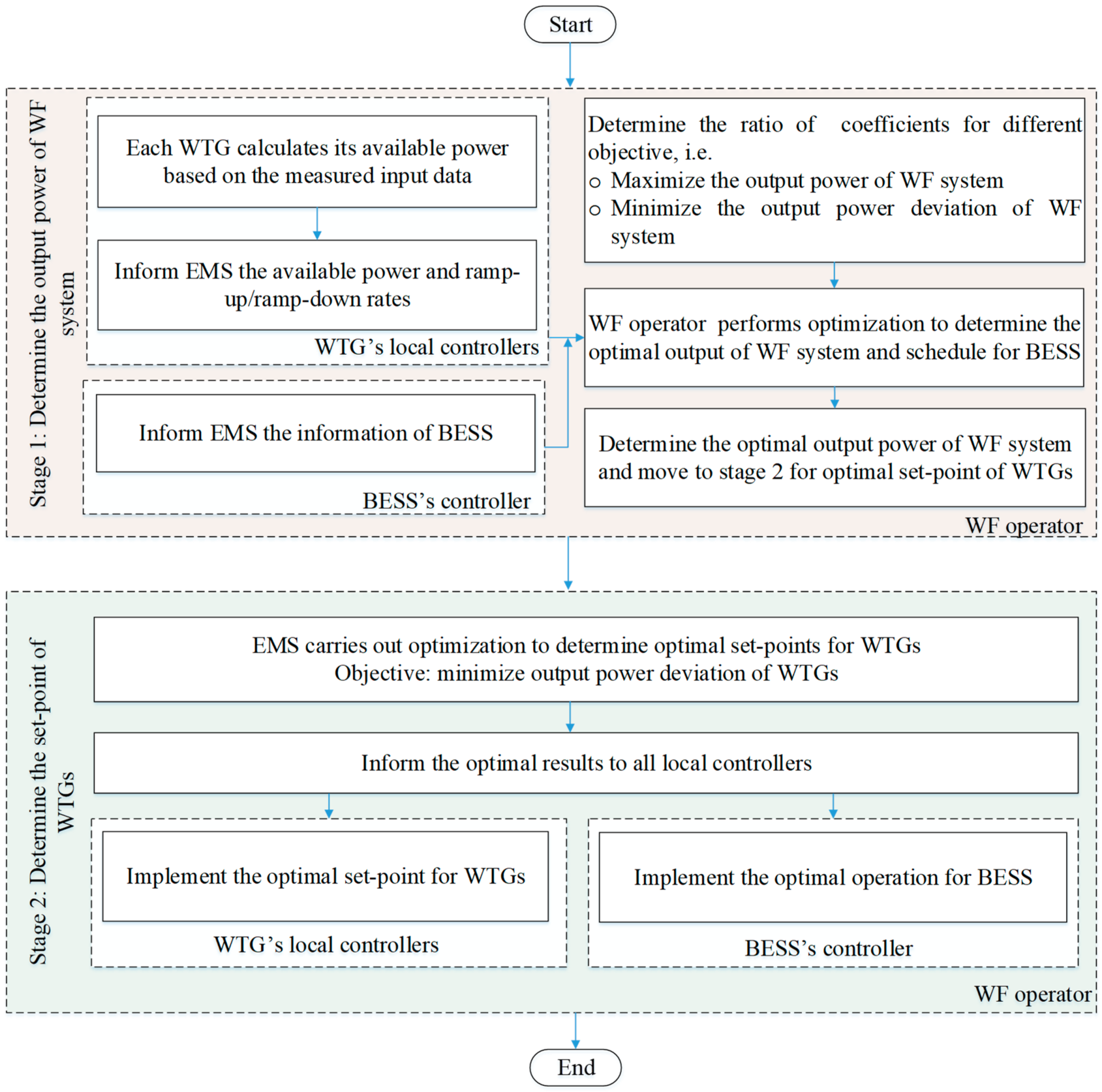
In this section, an operation strategy for the WF system is presented in detail, as shown in Figure 3. In this operation strategy, a two-stage optimization is proposed to optimize the operation of the WF system. As mentioned in the previous section, the operation of the WF system at MPPT can cause high fluctuations in output power. Therefore, in stage 1, the WF operator aims to determine the optimal output power from the WF system. Firstly, the WTG’s controllers calculate the maximum amount of power generation at the corresponding WTGs using relevant measurement information, such as wind speed, wind direction, and so on. Subsequently, local controllers will inform this information of maximum power to the WF operator. Similarly, if the WF system is equipped with BESS, the information related to BESS is also informed by the BESS’s controller to the WF operator. After gathering all information from local controllers, the WF operator will determine an optimal weighs’ ratio for the different objective functions based on the detailed analysis on the effect of different parameters on the operation of the WF system. Finally, the WF operator performs optimization using the above information to determine the optimal output power of the WF system.

In stage 2, the main concern is to determine the optimal set-point of WTGs to achieve the required output power of the WF system from stage 1. The determination of the objective function for stage 2 completely depends on the WF operator. Different WF operators often provide different objective functions for allocating the total required power to WTGs based on the WF system’s characteristics, e.g., on-shore/off-shore WF, type of WTGs, the position of WTGs, and so on. In this study, the objective function in stage 2 is to minimize the power deviation for the set-points of WTGs. This can help the output power of WTGs be smoother and thus avoid unnecessary internal fluctuations [31]. After the optimization process, the optimal set-points of WTGs and optimal schedule for BESS are determined. The WF operator will inform these optimal results to local controllers for implementation. The same process is repeated after each scheduling horizon. In WF operation, each scheduling horizon is usually set from a few hours to a day.

5. Mathematical Model

In this section, a mixed integer linear programming (MILP)-based optimization model is presented to optimize the operation of the WF system. In this paper, the main purpose is to optimize the operation of the WF system and WTGs. We assumed all WTGs are optimally placed in the WF area to minimize power losses due to the wake effect. Therefore, the wake model will not be presented in the optimization model. The optimization model is comprised of two stages, i.e., optimizing the output power of the WF system (stage 1) and optimizing the set-points of WTGs (stage 2). In state 1, a multi-objective optimization is introduced to determine the optimal output power for the WF system. The objective function (1) shows the profit of the WF system by selling power to the power system. The objective function (2) represents a penalty for output power fluctuation from the WF system. It can be realized that the two objective functions are conflicting, especially in the high variability of wind energy conditions. This leads to the necessity for developing a multi-objective optimization model to determine trade-off between two operation objectives. Various methods have been proposed to solve the multi-objective optimization problem, such as weighted sum method, goal programming, Pareto-based approaches, and so on [32]. Among these methods, the weighted sum method is a simple and widely applied method [33], which converts a multi-objective problem into a single objective problem by applying a function operator to the objective vector [32]. Therefore, we also develop a multi-objective function (3) by combining objective functions (1) and (2) with different weights using weighted sum method. This helps the WF operator for a trade-off between increasing output power and minimizing output power fluctuations. The relation between the weights of two different objective functions is shown in (4).

$$ProfitofWF={\displaystyle \sum _{t=1}^{T}P{R}_{sell,t}\cdot P_{out,t}}$$

(1)

$$Penaltyforpowerdeviation={\displaystyle \sum _{t=1}^{T}pe{n}_t\cdot \left|P_{out,t}-P_{out,t-1}\right|}$$

(2)

$$Max\left\{\alpha \cdot {\displaystyle \sum _{t=1}^{T}P{R}_{sell,t}\cdot P_{out,t}}-\beta \cdot {\displaystyle \sum _{t=1}^{T}pe{n}_t\cdot \left|P_{out,t}-P_{out,t-1}\right|}\right\}$$

(3)

$$\alpha +\beta =1$$

(4)

Objective (3) contains absolute values, and this makes it difficult to use MILP solvers, such as GAMS or CPLEX [31]. Therefore, a linearization is essential; additional variables are used to replace the absolute values, as shown in (5). The use of these additional variables requires two more constraints (6), (7) [34]. The output power of the WF system is bounded by (8).

$$Max\left\{\alpha \cdot {\displaystyle \sum _{t=1}^{T}P{R}_{sell,t}\cdot P_{out,t}}-\beta \cdot {\displaystyle \sum _{t=1}^{T}pe{n}_t\cdot D{P}_{out,t}}\right\}$$

(5)

$$D{P}_{out,t}\ge P_{out,t}-P_{out,t-1}\forall t\in T$$

(6)

$$D{P}_{out,t}\ge -\left(P_{out,t}-P_{out,t-1}\right)\forall t\in T$$

(7)

$$0\le P_{out,t}\le {\displaystyle \sum _{n=1}^N{P}_{n,t}^{avail}}\forall t\in T$$

(8)

However, when the WF system is equipped with a BESS. Objective function (3) is changed to (9), where the output power of the WF system is the sum of the output power of all WTGs and BESS, as given in (10). The main purpose of BESS is to reduce the output power fluctuations and keep the large power output of the WF system. Constraints related to the operation of the WF system are presented in (11) to (15). The charging bounds are shown in (11) considering SOC at the previous interval and the charging rate of BESS. Furthermore, in this paper, we assume that BESS can only charge power from the WF system, as given in (11). The discharging bounds are given in (12) considering the discharging rate and SOC of BESS at the previous interval. After determining the amount of charging/discharging power, SOC of BESS is updated using Equation (13). The initial value and the operation bounds of BESS are given in (14) and (15), respectively.

$$Max\left\{\alpha \cdot {\displaystyle \sum _{t=1}^{T}P{R}_{sell,t}\cdot P_{out\_total,t}}-\beta \cdot {\displaystyle \sum _{t=1}^{T}pe{n}_t\cdot \left|P_{out\_total,t}-P_{out\_total,t-1}\right|}\right\}$$

(9)

$$P_{out\_total,t}=P_{out,t}+P_t^{B-}-P_t^{B+}\forall t\in T$$

(10)

$$0\le P_t^{B+}\le \min \left\{P_{cap}^B\cdot \left(SO{C}_{\max }^B-SO{C}_{t-1}^B\right)\cdot \frac{1}{1-L^{B+}},P_{ramp,\max }^{B+},P_{out,t}^{}\right\}\forall t\in T$$

(11)

$$0\le P_t^{B-}\le \min \left\{P_{cap}^B\cdot \left(SO{C}_{t-1}^B-SO{C}_{\min }^B\right)\cdot (1-L^{B-}),P_{ramp,\max }^{B-}\right\}\forall t\in T$$

(12)

$$SO{C}_t^B=SO{C}_{t-1}^B-\frac{1}{P_{cap}^B}\cdot \left(\frac{1}{1-L^{B-}}\cdot P_t^{B-}-P_t^{B+}\cdot (1-L^{B+})\right)\forall t\in T$$

(13)

$$SO{C}_{t-1}^B=SO{C}_{ini}^{B}ift=1$$

(14)

$$SO{C}_{\min }^B\le SO{C}_t^B\le SO{C}_{\max }^B\forall t\in T$$

(15)

After stage 1, the optimal output power of the WF system is determined and taken as input data for stage 2. In stage 2, objective function (16) aims to determine the set-points of WTGs to minimize the power deviation inside the WF system. This helps to minimize the change in the output power of WTGs and reduce the fluctuations in the output power from the WTGs. Similar to stage 1, the objective function (16) also includes absolute values. A linearization is carried out using additional variables, as shown in (17). The additional constraints for linearization are presented in (18) to (21). The operation bounds of WTGs are presented in (22) considering the on/off status of WTGs. The available power of WTGs at each interval is calculated using (23) [35]. The power balance in the WF system is shown in (24). The total amount of power generation from all WTGs must be balanced with the amount of required output power from the WF operator determined in stage 1. Finally, constraints for ramp-up/ramp-down of WTGs is shown in (25) considering various parameters, i.e., the maximum amount for ramp-up/down, the minimum operation point of WTGs, the rated power, and the available power generation for WTGs.

$$Min\left\{{\displaystyle \sum _{\begin{array}{l}n=1\\ t=1\end{array}}^{N,T}pe{n}_{n,t}\cdot \left|P_{n,t}-P_{n,t-1}\right|}+{\displaystyle \sum _{\begin{array}{l}m,n=1\\ m\ne n\\ t=1\end{array}}^{N,T}pe{n}_{n-m,t}\cdot \left|P_{m,t}-P_{n,t}\right|}\right\}$$

(16)

$$Min\left\{{\displaystyle \sum _{\begin{array}{l}n=1\\ t=1\end{array}}^{N,T}pe{n}_{n,t}\cdot D{P}_{n,t}}+{\displaystyle \sum _{\begin{array}{l}m,n=1\\ m\ne n\\ t=1\end{array}}^{N,T}pe{n}_{n-m,t}\cdot D{P}_{n-m,t}}\right\}$$

(17)

$$D{P}_{n,t}\ge P_{n,t}-P_{n,t-1}\forall n\in N,t\in T$$

(18)

$$D{P}_{n,t}\ge -\left(P_{n,t}-P_{n,t-1}\right)\forall n\in N,t\in T$$

(19)

$$D{P}_{n-m,t}\ge P_{n-m,t}-P_{n-m,t}\forall n,m\in N,t\in T$$

(20)

$$D{P}_{n-m,t}\ge -\left(P_{n-m,t}-P_{n-m,t}\right)\forall n,m\in N,t\in T$$

(21)

$$s_{n,t}^{}.P_n^{\min }\le P_{n,t}^{}\le s_{n,t}^{}.\min \left\{P_n^{rate},P_{n,t}^{avail}\right\}\forall n\in N,t\in T$$

(22)

$$P_{n,t}^{avail}=\frac{1}{2}{C}_{p\_opt}\left({\beta }_{n,i},{\lambda }_{n,i}\right)\rho \pi R^2{v}_{n,t}^3\forall n\in N,t\in T$$

(23)

$${\displaystyle \sum _{n=1}^N{P}_{n,t}}=P_{out,t}^{stg1}\forall t\in T$$

(24)

$$s_{n,t+1}^{}.\max \left\{P_{n,t}-P_n^{RD},P_n^{\min }\right\}\le P_{n,t+1}\le s_{n,t+1}^{}.\min \left\{P_{n,t}+P_n^{RU},P_n^{rate},P_{n,t+1}^{avail}\right\}\forall n\in N,t\in T$$

(25)

In the next sections, the effects of different weights of objective functions and BESS size are analyzed in detail for stage 1. Different case studies are also presented to evaluate the effectiveness of the proposed method.

6. Numerical Results

The test WF system is comprised of 2 clusters, and each cluster is comprised of 5 WTGs in serial connection. The test system configuration is shown in Figure 4 based on the cluster project of the Korea Electric Power Corporation. All WTGs in the WF system have the same type and detailed information for the WTGs is presented as follows:

• The rated power is 10 MW;
• The minimum operation point is 10% of the rated power, i.e., 1 MW;
• The maximum ramp-up/down is 20% of the rated power, i.e., 2 MW.

The operation of the WF system is divided into different time windows, as shown in Figure 5. Each time window is 5 h long with 60 intervals, and each interval is set to 5 minutes. In each time window, the WF operator implements the optimal schedule, which has been determined in the previous time window and performs optimization to determine the optimal scheduling for the WF system in the next time window using the forecasting data. The entire two-stage optimization model is implemented in Visual Studio C++ integrated with IBM ILOG CPLEX 12.6 [36]. The IBM ILOG CPLEX Optimization Studio is an optimization software package and is widely used to determine the optimal solution for MILP-based models.

6.1. Input Data

In this section, input data is presented and used to evaluate the effectiveness of the proposed method. The proposed method can handle any input data of different time windows, e.g., day-time or night-time. Therefore, we only tested with a random time window. Figure 6a,b shows the available power of WTGs during a scheduling horizon (5 h in day-time) in clusters 1 and 2, respectively. The available power is estimated based on wind characteristics, i.e., wind speed, wind direction from the WF area. The set-point of each WTG can be adjusted from the minimum operation point (i.e., P_min) to the maximum operation point (i.e., the available power or MPPT) to meet the overall requirements for the entire WF system. The total amount of available power in the WF system is shown in Figure 6c. Finally, relevant information from the grid, such as the selling price and penalty signals is estimated based on the power sources and power demand profiles, as shown in Figure 6d.

6.2. Effect of α on the Output Power of WF System

In order to evaluate the effect of weight parameters in the multi-objective function, a detailed analysis is presented with different values of α. α represents the weight of the objective function (1) in the multi-objective function. This means that as the value of α increases, the WF operator will be more interested in increasing the output power of the WF system. It can be seen from Figure 7a that if the value of α increases, the amount of output power of the WF system also increases. The output power of the WF system is equal to the amount of available power when the value of α is 1. In contrast, when the value of α is close to 0, the WF operator only tries to minimize the output power fluctuation of the WF system. Therefore, the output power of the WF system is much smoother. Figure 7b shows the output power fluctuations from the WF system during the time window. It can be seen that the power fluctuation decreases significantly when the value of α is less than 0.4. However, this also significantly increases the amount of wind power curtailment, as shown in Figure 7c. Therefore, analyzing the effect of α helps the WF operator determines a trade-off between two operation objectives.

6.3. Effect of Ratio (β/α) on the Output Power of WF System

Similar to the previous section, we will analyze the effects of different weights on the operation of WF system. However, this section analyzes the effect of ratio (β/α) on optimal results. Therefore, the WF operator can determine a ratio (β/α) for trade-off between different operation objectives. The values of the weights α, β are shown in Figure 8a with different ratios. The total amount of output energy of the WF system and the total amount of wind energy curtailment are shown in Figure 8b during the scheduling horizon. It can be observed that the amount of output energy and wind energy curtailment do not change significantly when the value of ratio is greater than 2 in this case study. Depending on different WF systems, the WF operators will choose an optimal ratio for the operation of WF systems.

6.4. Effect of BESS Size on the Output Power of WF System

In the previous section, we only analyzed the effects of different weights of objective functions on the operation of the WF system without any energy storage system. However, BESS has recently been used in the operation of WF systems for different purposes, e.g., smoothing out the output power, increasing the output power of the WF system. In this case, we assume that the weight ratio (β/α) is set to 0.5/0.5 to analyze the effect of BESS size on the operation of the WF system in detail.

Figure 9a shows the output power of the WF system with different BESS size. It can be observed from Figure 9a that the output power of the WF system increases significantly if the size of BESS increases. The use of BESS can help the WF system shifts power from peak output intervals to off-peak output intervals. Therefore, using BESS not only helps increase the output power of the WF system but also significantly reduces the output power fluctuations. Increasing the size of the BESS also reduces the output power fluctuation of the WF system, as shown in Figure 9b. Figure 9c shows the total output energy of the WF system and the total wind energy curtailment during the scheduling horizon. If the size of the BESS is about 80 MW, the total output energy of the WF system does not change significantly in this case study.

6.5. Effect of Both Ratio (β/α) and BESS Size on the Output Power of WF System

In this section, we will analyze in detail the effect of both weight ratio (β/α) and BESS size on the operation of the WF system. Figure 10a,b shows the total amount of WF’s output energy during the scheduling horizon in front view and top view, respectively. It can be observed that the amount of energy gained from the WF system increases when the weight ratio decreases and the size of the BESS increases. When the value of weight ratio is close to 0, the effect of BESS size is negligible because the WF operator always operate the WF system at MPPT. Conversely, when the BESS size is increased, the effect of weight ratio is also decreased.

Similarly, Figure 11a,b shows the total amount of wind energy curtailment during the scheduling horizon in front view and top view, respectively. The total curtailment amount of wind energy is high when the value of the weight ratio is greater than 2 and BESS is small. It can be observed that increasing the BESS size or decreasing the weight ratio can significantly reduce the wind energy curtailment in the WF system.

6.6. Optimal Set-Point of WTGs in Different Case Studies

In the previous section, detailed analyses on the effect of various parameters on the operation of the WF system have been presented. Based on the input data, the WF operator can easily determine the optimal operation point for the WF system (i.e., stage 1). After determining the optimal operation point for the WF system, the WF operator also performs optimization (i.e., stage 2) to determine the optimal set-points of WTGs to fulfill the operation point of the WF system taken from stage 1. By using the proposed method, the amount of power deviation for the set-points of WTGs can also be significantly reduced. This can help WF systems avoid unnecessary power fluctuations. In the next section, two different case studies will be presented in detail to demonstrate the effectiveness of the proposed method.

6.6.1. Case study 1: Ratio (β/α) is 0.5/0.5 and without BESS

In case the ratio (β/α) is 0.5/0.5, the WF operator will perform optimization and determine the optimal output power for the WF system. It can be observed from Figure 12 that the amount of output power of the WF system is reduced, but the fluctuation of the output power of the WF system is also significantly reduced. After determining the optimal output power of the WF system, the WF operator also performs optimization to minimize the amount of power deviation for the set-points of WTGs. Figure 13a,b shows the optimal set-points of WTGs in cluster 1 and cluster 2, respectively. It can be seen that the outputs of WTGs are smoother by determining the optimal set-points of WTGs within [P_min, P_max].

6.6.2. Case study 2: Ratio (β/α) is 0.5/0.5 and BESS size is 40 MW

Similar to the previous section, a two-stage optimization is used to determine the optimal output power of the WF system and the optimal set-points of WTGs. The use of BESS enables the WF system to generate more output power and also reducing the fluctuations in output power from the WF system compared to the first case study. The purpose of BESS is to shift power from peak output intervals to off-peak output intervals to reduce fluctuations in output power from the WF system. It can be observed from Figure 14 that the output power of the WF system increases significantly when using BESS. This output power of the WF system is almost equal to the maximum output power from the WF system. If the size of BESS is large enough, the amount of output power can be equal to the maximum output of the WF system. The total selling power from the WF system to the power system in each interval is the total output power from the WF and the charge/discharge power from BESS. Figure 15a,b shows the optimal set-points of WTGs in cluster 1 and cluster 2, respectively. Due to the increase in output power of the WF system (almost equal to the maximum output power), the set-points of WTGs are also near to the amount of available power shown in Figure 6a,b.

7. Discussion on Future Extension of This Study

In this study, we propose a multi-objective optimization method for the operation of the WF system. By using the proposed method, the WF operator can determine the optimal operation point for the WF system as well as optimal set-points for WTGs. Although many case studies have been analyzed in detail, there are still some other aspects that have not considered in this study. For example, the impact of the operation of the upstream WTGs on the operation of the downstream WTGs, i.e., wake model is required to analyze in detail to determine an optimal operation point for each WTGs for reducing the amount of power losses in the WF system. In addition, a forecasting model is necessary to predict the available output power of WTGs based on measurement information such as wind speed, wind direction, as well as the market price signals using the history data. However, it is impossible to accurately predict the above parameters. Therefore, the forecasting values with uncertainty bounds are required for the operation of the WF system. These uncertainties may have adverse effects on the operation of the WF system, e.g., reducing the service reliability. Therefore, uncertainty analysis is necessary to be present in detail. Finally, a suitable comparison with other studies is also required to show the advantages of the proposed method in the operation of the WF system. The above aspects are suitable future extensions for this study.

8. Conclusions

In this paper, a multi-objective optimization method has been proposed for determining a trade-off between maximizing the output power and minimizing power fluctuation of WF systems. The effects of different weight ratios (β/α) and BESS size on the operation of the WF system have been analyzed in detail. Based on the analysis, it can be concluded that in order to balance between output power amount and output power quality of the WF system, the weight ratio should be greater than 1, and BESS size should be greater than 40MW for the test WF system with total capacity as 100 MW. In additional, several case studies have also been carried out to show the effectiveness of the proposed method. In all case studies, a two-stage optimization has been used to determine the optimal output power of the WF system and the optimal set-points of WTGs. In stage 1, the multi-objective optimization has been solved to determine the optimal operation point of the WF system, which helps the WF system to balance its profit and output power quality. Especially, the use of BESS can significantly increase the output power of the WF system, while simultaneously preserving a high output power quality of the WF system. In stage 2, the optimal operation of WTGs is determined to minimize the power deviation for the set-points of WTGs and achieve the optimal operation point from stage 1. It can be seen that the power deviation for the set-points of WTGs has been significantly reduced. This helps the output power of WTGs much smoother and, therefore, avoids unnecessary power fluctuations inside the WF system.