Frequency Adaptive Current Control Scheme for Grid-connected Inverter without Grid Voltage Sensors Based on Gradient Steepest Descent Method

Abstract

This paper presents a frequency adaptive grid voltage sensorless control scheme of a grid-connected inductive–capacitive–inductive (LCL)-filtered inverter, which is based on an adaptive current controller and a grid voltage observer. The frequency adaptive current controller is constructed by a full-state feedback regulator with the augmentation of multiple control terms to restrain not only the inherent resonance phenomenon that is caused by LCL filter, but also current harmonic distortions from an adverse grid environment. The number of required sensing devices is minimized in the proposed scheme by means of a discrete-time current-type observer, which estimates the system state variables, and gradient-method-based observers, which estimate the grid voltages and frequency simultaneously at different grid conditions. The estimated grid frequency is utilized in the current control loop to provide high-quality grid-injected currents, even under harmonic distortions and the frequency variation of grid voltages. As a result, the grid frequency adaptive control performance as well as the robustness against distorted grid voltages can be realized. Finally, an inverter synchronization task without using grid voltage sensors is accomplished by a fundamental grid voltage filter and a phase-locked loop to detect the actual grid phase angle. The stability and convergence performance of the proposed observers have been studied by means of the Lyapunov theory to ensure a high accuracy tracking performance of estimated variables. Simulation and experimental results are presented to validate the feasibility and the effectiveness of the proposed control approach.

1. Introduction

The distributed generation (DG) employing renewable energy from wind or solar sources has gained a lot of interest from energy producers and consumers, owing to environment-friendly features [1]. Enhancing the reliability, efficiency, and competitive cost are highly desirable in constructing the DG system to maximize the potential of renewable energy in the electrical energy demand. In this respect, a voltage source inverter (VSI) plays an important role as an interface between the DG and the main grid [2]. The control performance of a grid-connected inverter should be robust against the negative effects from the main grid, such as the harmonic distortion or the grid frequency deviation, to inject the active power from DG to the grid with high-quality injected currents, which complies with the restricted grid codes [3].

Most grid-connected inverter topologies use the pulse width modulation (PWM) technique with a high switching frequency to reduce the harmonic contents in output voltages. As a result, output low-pass filters should be connected between inverters and grid to attenuate high frequency harmonics. There are three main filter alternatives, known as inductor (L), inductor-capacitor-inductor (LCL), and inductor-capacitor (LC) filters. Among them, the LCL filter configuration is a preferable option due to its better performance in terms of higher harmonic attenuation with a smaller inductor size and cost in comparison with the conventional L or LC filter [4,5,6]. However, complicated dynamic characteristics, as well as the risk of resonance phenomenon in LCL filters, pose a challenge in the controller design for stabilizing the system.

A resonance damping method is normally required to control the LCL-filtered inverter system. The damping techniques can be generally categorized into two methods: the passive damping by using additional physical components on LCL circuits and the active damping by implementing current control algorithms. Even though the passive damping is simple, the extra loss through heat dissipation is unavoidable [7]. On the other hand, since the active damping method can be realized without extra loss, this scheme has been widely adopted to stabilize the inverter system at the expense of increased computational burden and additional sensing devices [8,9,10]. Particularly, the research work in [9] uses the capacitor current feedback to realize the virtual-resistor-based active damping concept. The current controller is modified by including the feedback of filter capacitor voltages to achieve the resonance damping in other approaches that were introduced in [8,10]. Obviously, both of these methods require extra sensors. Alternatively, the studies in [11,12] introduce a state-space control method for an LCL-filtered inverter system, in which the closed-loop poles can be placed at the desired locations to damp the resonance peak. These research works implement a full-state observer to estimate the system state variables instead of using direct measurements.

Many researchers put effort towards eliminating more sensors in system for the purpose of reducing the cost and hardware complexity of a grid-connected inverter. As the DC-link voltage and grid-side currents are essential for the protection against over voltage and over current, these sensors cannot be removed. Another approach is to eliminate grid voltage sensors that measure grid voltages to extract the information for synchronizing the DG system with main grid. To realize the synchronization of DG system with the main grid without grid voltage measurements, several grid voltage sensorless control schemes have been reported. In [13], the grid voltages are algebraically deduced from inverter voltages and voltages drop in the filter inductors, in which quadrature low-pass filters are adopted to accomplish the required differentiation operation with currents. This method is simple and it has low computational burden. However, it is only applicable for L-filtered inverter systems. The concept of the virtual flux estimator is applied to realize a voltage sensorless control for an LCL-filtered inverter [14]. In [15], a disturbance voltage model is augmented into the state-space model of a PWM converter system to estimate the line voltage waveforms.

The aforementioned methods use the precise knowledge on the grid frequency in the design of grid voltage sensorless control schemes. However, in the weak grid condition, the grid frequency is time-varying, causing the degradation or even instability in operation of control and estimation algorithms. The sensorless control scheme should be able to produce desirable harmonic-free injected currents by adapting to the grid frequency deviation to meet the requirement of robustness against both the distorted grid and frequency variation in the grid-connected inverter. The study in [16] presents a voltage sensorless scheme based on the sliding mode observer to control a three-phase voltage source rectifier under unbalanced grid conditions. Though a good performance is achieved under several adverse test conditions by this approach, the grid frequency that was obtained by the conventional phase-locked loop (PLL) still has long transient time under a sudden frequency step change. A closed-loop observer-based grid voltage sensorless control scheme is introduced for a VSI with L and LCL filters in [17] and [18], respectively. In these schemes, the grid frequency in the disturbance model is tuned online by means of grid frequency estimators. However, these schemes require quite heavy computational burden since all the harmonic components in the distorted grid condition should be included into system model in order to ensure good convergence of the estimated voltages to the actual quantities. Another approach in [19] presents a model reference adaptive control structure by using the active- and reactive-power model to estimate the grid voltages. The PLL is eliminated in this estimation algorithm owing to the exactness of the extracted grid frequency and phase angle information.

Recently, optimization algorithms have been investigated and adopted into several applications due to their high efficiency and low computational burden features, in which the unknown system parameters are iteratively estimated to minimize the parameter estimation error [20,21,22,23]. In particular, the research in [20] presents a neural adaptive notch filter for an active power filter, in which the least-mean-square algorithm is adopted for updating the weights of the adaptive neural harmonic estimator. In [21,22], the grid voltages are estimated by using the estimator based on a gradient steepest descent method for L- and LCL-filtered inverters, respectively. However, these schemes did not consider the grid frequency variation in controller design. Alternatively, a voltage estimation scheme that is based on the Newton–Raphson optimization technique is presented in [23]. This approach utilizes the exchanged power models between VSI and the main grid via an L filter to formulate the optimization problem in terms of unknown grid information. However, this algorithm is still not suitable for estimating the grid voltages for an LCL-filtered inverter model.

In this paper, a frequency adaptive current control scheme without grid voltage sensors is presented for a grid-connected LCL-filtered inverter. A current controller presented in [24] is applied, which includes a full-state feedback regulator and multiple augmented control terms, in order to stabilize the inverter system and to fulfill control objectives such as the zero steady-state reference tracking error and the harmonic disturbance compensation under adverse grid conditions. To reduce the system cost as well as the hardware complexity, only the measurement of DC-link voltage and grid-side currents are used in the design of the proposed control scheme. Instead, two observers are simultaneously employed to reliably estimate both system state variables and grid voltages. Particularly, a discrete current-type observer is constructed to estimate the system states, while the grid voltages are precisely estimated by an adaptive observer based on the gradient steepest descent method. The uncertainty in the main grid, such as the grid frequency variation and harmonic distortion, poses a challenge for the synchronization task of the voltage sensorless control scheme. To overcome this issue, a resonant filter in the discrete-time state-space tuned at the fundamental frequency cooperated with the conventional PLL scheme to restrain the effect of the harmonic distortion on the extracted grid phase angle. Furthermore, since the exact grid frequency information is essential to tune the frequency adaptive current controller as well as the resonant filter, this paper also proposes a novel grid frequency estimator that is based on the least-mean-square algorithm to produce the frequency estimate with low variation and fast convergence features. The PSIM software-based simulations (9.1, Powersim, Rockville, MD, USA) and experiments have been carried out comprehensively by using a three-phase 2 kVA prototype grid-connected inverter under adverse grid conditions to demonstrate the effectiveness and the feasibility of the proposed frequency adaptive voltage sensorless control scheme. As a result, the proposed current controller has robustness against negative impacts from grid, such as the harmonic distortion and the grid frequency variation, even without grid voltage sensors.

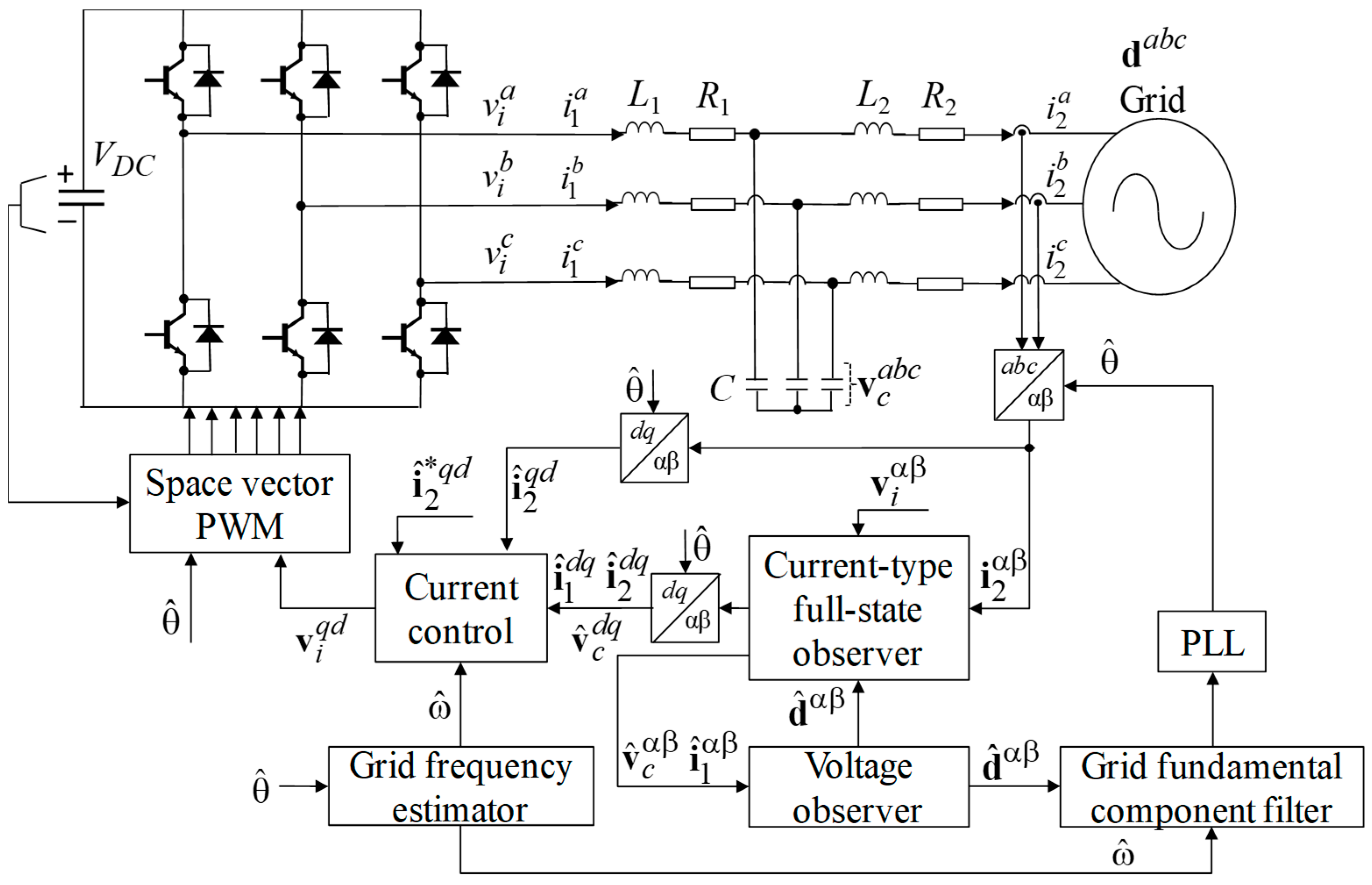
2. System Description

Figure 1 depicts a configuration of a three-phase grid-connected VSI with LCL filter, where R₁, L₁, R₂, and L₂ denote resistances and inductances of the filter in the converter-side and the grid-side, respectively, and C represents the filter capacitance. The proposed control scheme is constructed by a robust current controller and multiple observers that estimate both system state variables and grid voltages in order to inject high-quality currents into the grid with utilizing only grid-side current and DC-link voltage sensors. In particular, the estimated quantities of grid-side currents ${\widehat{i}}_2$, inverter-side currents ${\widehat{i}}_1$, and capacitor voltages ${\widehat{v}}_c$ are obtained from the current-type full-state observer to feed them to the current controller. The variable $\widehat{d}$ denotes the estimated quantities of grid voltages, which is updated online from the gradient-method-based observer. The synchronization task of the inverter and the main grid is accomplished by a PLL with the fundamental grid voltages being extracted from a grid fundamental component filter. The estimated grid frequency $\widehat{\mathsf{\omega }}$ obtained from the proposed grid frequency estimator is fed back to the current controller and the grid fundamental component filter to realize the frequency adaptive scheme. Finally, the reference voltages v_i as the output of the current controller are modulated by the space vector pulse width modulation (SVPWM) method.

The mathematical model of the inverter system in the natural reference frame can be written for phase a, as

$$\frac{d}{dt}{i}_1^a(t)=-\frac{R_1}{L_1}{i}_1^a(t)+\frac{1}{L_1}{v}_i^a(t)-\frac{1}{L_1}{v}_c^a(t)$$

(1)

$$\frac{d}{dt}{i}_2^a(t)=-\frac{R_2}{L_2}{i}_2^a(t)+\frac{1}{L_2}{v}_c^a(t)-\frac{1}{L_2}{d}^a(t)$$

(2)

$$\frac{d}{dt}{v}_c^a(t)=\frac{1}{C}{i}_1^a(t)-\frac{1}{C}{i}_2^a(t)$$

(3)

where the superscript “a” denotes phase-a variables, i₁, i₂, and v_c denote the inverter-side current, the grid-side current, and the capacitor voltage, respectively, v_i is the inverter voltage, and d denotes the grid voltage. Similar equations are applied for phase b and c.

3. Proposed Frequency Adaptive Current Control Scheme Without Voltage Sensors

In this section, the proposed frequency adaptive sensorless current control scheme is presented in detail. A current controller is first constructed in the synchronous reference frame (SRF) to stabilize the LCL-filtered inverter system and to achieve main control objectives such as the reference tracking and the disturbance compensation. Two observers are constructed in the stationary frame to obtain the estimates for system state variables and grid voltages to realize a grid voltage sensorless control scheme. It is worth to note that since the system models in α-axis and β-axis are independent of each other, the observers are designed by only considering the system model in α-axis and it is then similarly applied to the system model in the β-axis. A novel grid frequency estimator is also introduced to estimate the actual grid frequency by online, and the estimated grid frequency is fed back to the current controller. Finally, the synchronization issue is discussed to ensure a safe and reliable connection between the DG and the main grid.

3.1. Frequency Adaptive Current Controller

The current controller is designed by a full-state feedback regulator with the augmentation of an integral term and two resonant terms tuned at interesting harmonic components into inverter system model [24]. In the SRF, the reference tracking of grid-side current is easily achieved by means of a simple integral control term. Additionally, four harmonic components in phase currents at the 5th, 7th, 11th, and 13th orders can be effectively compensated at the same time with only two resonant terms at 6th and 12th orders in the SRF. Therefore, the computational burden of the current controller is reduced in the SRF as compared to other approaches that were implemented in the stationary frame.

The mathematical model of the inverter system can be expressed in the SRF by means of the Park’s transformation, as follows:

$$\frac{d}{dt}{i}_2^q(t)=-\frac{R_2}{L_2}{i}_2^q(t)-\mathsf{\omega }{i}_2^d(t)+\frac{1}{L_2}{v}_c^q(t)-\frac{1}{L_2}{d}^q(t)$$

(4)

$$\frac{d}{dt}{i}_2^d(t)=-\frac{R_2}{L_2}{i}_2^d(t)+\mathsf{\omega }{i}_2^q(t)+\frac{1}{L_2}{v}_c^d(t)-\frac{1}{L_2}{d}^d(t)$$

(5)

$$\frac{d}{dt}{i}_1^q(t)=-\frac{R_1}{L_1}{i}_1^q(t)-\mathsf{\omega }{i}_1^d(t)-\frac{1}{L_1}{v}_c^q(t)+\frac{1}{L_1}{v}_i^q(t)$$

(6)

$$\frac{d}{dt}{i}_1^d(t)=-\frac{R_1}{L_1}{i}_1^d(t)+\mathsf{\omega }{i}_1^q(t)-\frac{1}{L_1}{v}_c^d(t)+\frac{1}{L_1}{v}_i^d(t)$$

(7)

$$\frac{d}{dt}{v}_c^q(t)=-\mathsf{\omega }{v}_c^d(t)-\frac{1}{C}{i}_2^q(t)+\frac{1}{C}{i}_1^q(t)$$

(8)

$$\frac{d}{dt}{v}_c^d(t)=\mathsf{\omega }{v}_c^q(t)-\frac{1}{C}{i}_2^d(t)+\frac{1}{C}{i}_1^d(t)$$

(9)

where the superscript “q” and “d” denote the q-axis and d-axis variables, respectively, and ω is the grid angular frequency. From Equation (4) to (9), the continuous-time representation of system can be expressed in a state-space model, as

$$\dot{x}(t)=Ax(t)+Bu(t)+Dd(t)$$

(10)

$$y(t)=Cx(t)$$

(11)

where $x={[i_2^q\hspace{0.17em}\hspace{0.17em}{i}_2^d\hspace{0.17em}\hspace{0.17em}{i}_1^q\hspace{0.17em}\hspace{0.17em}{i}_1^d\hspace{0.17em}\hspace{0.17em}{v}_c^q\hspace{0.17em}\hspace{0.17em}{v}_c^q]}^T$ is the system state vector, $u={[v_i^q\hspace{0.17em}\hspace{0.17em}{v}_i^d]}^T$ is the system input vector, $d={[d^q\hspace{0.17em}\hspace{0.17em}{d}^d]}^T$ is the grid voltage vector, and the system matrices A, B, C, and D are presented, as

$$A=\left[\begin{array}{cccccc}-R_2/L_2& -\mathsf{\omega }& 0& 0& 1/L_2& 0\\ \mathsf{\omega }& -R_2/L_2& 0& 0& 0& 1/L_2\\ 0& 0& -R_1/L_1& -\mathsf{\omega }& -1/L_1& 0\\ 0& 0& \mathsf{\omega }& -R_1/L_1& 0& -1/L_1\\ -1/C& 0& 1/C& 0& 0& -\mathsf{\omega }\\ 0& -1/C& 0& 1/C& \mathsf{\omega }& 0\end{array}\right],\hspace{0.17em}\hspace{0.17em}B=\left[\begin{array}{cc}0& 0\\ 0& 0\\ 1/L_1& 0\\ 0& 1/L_1\\ 0& 0\\ 0& 0\end{array}\right]$$

(12)

$$D=\left[\begin{array}{cc}-1/L_2& 0\\ 0& -1/L_2\\ 0& 0\\ 0& 0\\ 0& 0\\ 0& 0\end{array}\right],\hspace{0.17em}\hspace{0.17em}C=\left[\begin{array}{cccccc}1& 0& 0& 0& 0& 0\\ 0& 1& 0& 0& 0& 0\end{array}\right]$$

(13)

For a digital implementation of the current controller, the system model can be transformed into the discrete-time domain by using the zero-order hold (ZOH) method with the sampling time T_s, as [25]

$$x(k+1)=A_{d}x(k)+B_{d}u(k)+D_{d}d(k)$$

(14)

$$y(k)=C_{d}x(k)$$

(15)

where the matrices A_d, B_d, D_d, and C_d can be calculated as

$$A_d=e^{A{T}_s},\hspace{1em}{B}_d=\left({\displaystyle {\int }_0^{T_s}{e}^{At}dt}\right)B,\hspace{1em}{D}_d=\left({\displaystyle {\int }_0^{T_s}{e}^{At}dt}\right)D,\hspace{1em}{C}_d=C.$$

(16)

Figure 2 represents the detailed block diagram of the proposed current controller, in which the control input u(k) is computed from the output of the full-state feedback regulator, the integral control term, and two resonant terms that were tuned at 6ω and 12ω.

The integral control term is expressed in the discrete-time state-space model, as [24,25]

$$z_0(k+1)=A_P{z}_0(k)+B_P\mathsf{\epsilon }(k)$$

(17)

where $A_P=I_{2\times 2}$, $B_P=T_s\times I_{2\times 2}$, $z_0(t)={\left[\begin{array}{cc}{z}_0^q(k)& z_0^d(k)\end{array}\right]}^T$ is the state vector of integral control term, $\mathsf{\epsilon }(k)={\left[\begin{array}{cc}{\mathsf{\epsilon }}^q(k)& {\mathsf{\epsilon }}^d(k)\end{array}\right]}^T=r(k)-C_{d}x(k)$ is the current error vector, $r(k)={\left[\begin{array}{cc}{i}_2^{q*}(k)& i_2^{d*}(k)\end{array}\right]}^T$ is the reference current vector.

For the purpose of compensating the harmonic distortion at 5^th, 7^th, 11^th, and 13^th orders from the adverse grid environment, the current controller augments the frequency adaptive resonant control terms tuned at 6ω and 12ω, as [24,26]

$$\left[\begin{array}{c}{\delta }_1(k+1)\\ {\delta }_2(k+1)\end{array}\right]=A_{rn}^s\left[\begin{array}{c}{\delta }_1(k)\\ {\delta }_2(k)\end{array}\right]+B_{rn}^s\mathsf{\epsilon }(k)$$

(18)

where $A_{rn}^s=\left[\begin{array}{cc}2\cos (n\mathsf{\omega }{T}_s)& 1\\ -1& 0\end{array}\right],\hspace{0.17em}{B}_{rn}^s=\left[\begin{array}{c}\cos (n\mathsf{\omega }{T}_s)\\ -1\end{array}\right]$.

By using the discrete-time state-space model for the resonant control in (18), the grid frequency can be updated online when the actual grid frequency varies. As a result, the distorted harmonics are effectively attenuated, even under the grid frequency deviation. Applying resonant control terms for q-axis and d-axis of $\mathsf{\epsilon }(k)$ yields

$$z_n(k+1)=A_{rn}{z}_n(k)+B_{rn}\mathsf{\epsilon }(k)$$

(19)

where $z_n={[\begin{array}{cccc}{\delta }_{1n}^q& {\delta }_{2n}^q& {\delta }_{1n}^d& {\delta }_{2n}^d\end{array}]}^T$, $A_{rn}=\left[\begin{array}{cc}{A}_{rn}^s& 0_{2\times 2}\\ 0_{2\times 2}& A_{rn}^s\end{array}\right]$, and $B_{rn}=\left[\begin{array}{cc}{B}_{rn}^s& 0_{2\times 1}\\ 0_{2\times 1}& B_{rn}^s\end{array}\right]$.

The above integral in (17) and resonant control terms in (19) are augmented into the system model to design full-state feedback regulation, as follows:

$$x_e(k+1)=A_e{x}_e(k)+B_{e}u(k)+D_{e}d(k)+B_{re}r(k)$$

(20)

$$y(k)=C_e{x}_e(k)$$

(21)

$$u(k)=-K{x}_e(k)$$

(22)

where $x_e=[\begin{array}{cccc}{x}^T& z_0^T& z_6^T& z_{12}^T\end{array}]{\hspace{0.17em}}^T$, $A_e=\left[\begin{array}{cccc}{A}_d& 0_{6\times 2}& 0_{6\times 4}& 0_{6\times 4}\\ -B_P{C}_d& A_P& 0_{2\times 4}& 0_{2\times 4}\\ -B_{r6}{C}_d& 0_{4\times 2}& A_{r6}& 0_{4\times 4}\\ -B_{r12}{C}_d& 0_{4\times 2}& 0_{4\times 4}& A_{r12}\end{array}\right]$, $B_e=\left[\begin{array}{c}{B}_d\\ 0_{2\times 2}\\ 0_{4\times 2}\\ 0_{4\times 2}\end{array}\right]$, $D_e=\left[\begin{array}{c}{D}_d\\ 0_{2\times 2}\\ 0_{4\times 2}\\ 0_{4\times 2}\end{array}\right]$, $B_{re}=\left[\begin{array}{c}{0}_{6\times 2}\\ B_P\\ B_{r6}\\ B_{r12}\end{array}\right]$ $C_e=[\begin{array}{cccc}{C}_d& 0_{2\times 2}& 0_{2\times 4}& 0_{2\times 4}\end{array}]$, $K=[\begin{array}{cccc}{K}_x& K_{Pz}& K_{6z}& K_{12z}\end{array}]$, with K_x $\in$ ℜ^2×6, K_Pz $\in$ ℜ^2x2, K_6z $\in$ ℜ^2x4, and K_12z $\in$ ℜ^2x4. The feedback gain matrix K in (22) should be chosen to ensure the stability of the current control scheme. In this study, a linear quadratic regulation (LQR) approach is applied to select an optimal feedback gain matrix systematically [25].

3.2. Discrete-Time Current-Type Full State Observer

In the proposed current controller (20)-(22), all of the system state variables should be available to determine the control input by the full-state feedback. However, only grid-side currents and the DC-link voltage are directly measured to reduce the cost and hardware complexity due to sensing devices. A full-state observer is employed to produce the estimated signals for grid-side currents, inverter-side currents, and capacitor voltages. As detailed discussions in [12,24,27], the discrete-time current-type observer is chosen in this study to enhance the stability of observer under different operation conditions.

The inverter model representation in the stationary reference frame is chosen to construct the full-state observer. From (1)-(3), the inverter model transformed to the stationary reference frame is obtained, as

$${\dot{x}}_s^{\alpha }(t)=A_{sc}{x}_s^{\alpha }(t)+B_{sc}{v}_i^{\alpha }(t)+D_{sc}{d}^{\alpha }(t)$$

(23)

$$y^{\alpha }(t)=C_{sc}{x}_s^{\alpha }(t)$$

(24)

where $x_s^{\alpha }={[\begin{array}{ccc}{i}_1^{\alpha }& v_c^{\alpha }& i_2^{\alpha }\end{array}]}^T$, $A_{sc}=\left[\begin{array}{ccc}-R_1/L_1& -1/L_1& 0\\ 1/C& 0& -1/C\\ 0& 1/L_2& -R_2/L_2\end{array}\right]$, $B_{sc}\left[\begin{array}{c}1/L_1\\ 0\\ 0\end{array}\right]$, and $D_{sc}=\left[\begin{array}{c}0\\ 0\\ -1/L_2\end{array}\right]$.

Obviously, the system model in (23) and (24) does not contain the grid frequency information as the system model (10)-(11) in the SRF. As a result, the frequency variation do not affect the estimation performance of the proposed observer.

To construct the full-state observer in the discrete-time domain, the inverter system model in (23)-(24) is discretized by the offline ZOH method, as follows:

$$x_s^{\alpha }(k+1)=A_{sd}{x}_s^{\alpha }(k)+B_{sd}{v}_i(k)+D_{sd}{d}^{\alpha }(k)$$

(25)

$$y(k)=C_{sd}{x}_s(k)$$

(26)

where A_sd, B_sd, C_sd, D_sd is the discrete-time counterparts of A_sc, B_sc, C_sc, D_sc, respectively. From (25) and (26), the current full-state observer is given as

$${\widehat{x}}^{-}{}^{\alpha }(k+1)=A_{sd}{\widehat{x}}^{\alpha }(k)+B_{sd}{v}_i^{\alpha }(k)+D_{sd}{\widehat{d}}^{\alpha }(k)$$

(27)

$${\widehat{x}}^{\alpha }(k+1)={\widehat{x}}^{-\alpha }(k+1)+K_e[y^{\alpha }(k+1)-C_d{\widehat{x}}^{-\alpha }(k+1)]$$

(28)

where the superscript “α” denotes the α-axis, ${\widehat{x}}^{\alpha }$ is the estimated current state vector, and K_e is the observer gain matrix. ${\widehat{x}}^{-\alpha }$ is the computed state vector from the system dynamic model and the input signal $v_i^{\alpha }$ at time step k in (27). The estimated vector ${\widehat{x}}^{\alpha }$ is calculated by the ${\widehat{x}}^{-\alpha }$ and a correction term at time step (k + 1) in Equation (28). It is worth noting that the grid voltage is unknown in a grid voltage sensorless control scheme.

The grid voltage is estimated by the gradient-based observer in order to avoid the steady-state error in the estimated state variables, as presented in the next section and the estimated grid voltage ${\widehat{d}}^{\alpha }$ is updated in (27). If the estimated grid voltage converges well to the actual value, then the error dynamics of the observer can be obtained by subtracting (28) from (25), as follows:

$${\tilde{x}}^{\alpha }(k+1)=x^{\alpha }(k+1)-{\widehat{x}}^{\alpha }(k+1)=(A_{sd}-K_e{C}_{sd}{A}_{sd}){\tilde{x}}^{\alpha }(k).$$

(29)

The observer gain matrix K_e should be selected in order that the eigenvalues of $(A_{sd}-K_e{C}_{sd}{A}_{sd})$ are placed inside the unit circle. Subsequently, the estimation error tends to zero or the estimated states converge to the actual ones. The observer gain matrix can be selected by applying the similar LQR approach as the current control design.

3.3. Adaptive Gradient Steepest Descent Method for Grid Voltage Estimation

In this section, a simple and effective gradient steepest descent-based observer is presented to estimate the grid voltage with low computational burden. Suppose that the inverter-side currents and capacitor voltages are reliably estimated by the discrete-time current-type observer. These estimated values and inverter voltages are fed to the dynamic model of grid-side current to estimate the grid voltage, as shown in Figure 3.

To estimate an unknown grid voltage in the α-axis, an adaptive observer is constructed with open loop structure, as follows:

$${\overline{i}}_2^{\alpha }(k+1)=C_{sd}{A}_{sd}{\overline{x}}_s^{\alpha }(k)+C_{sd}{B}_{sd}{v}_i^{\alpha }(k)+C_{sd}{D}_{sd}{\widehat{d}}^{\alpha }(k)$$

(30)

where ${\overline{x}}_s^{\alpha }(k)={[\begin{array}{ccc}{\widehat{i}}_1^{\alpha }& {\widehat{v}}_c^{\alpha }& {\overline{i}}_2^{\alpha }\end{array}]}^T$ and ${\overline{i}}_2^{\alpha }$ is the estimated grid-side current by the proposed adaptive observer. With the same inverter input voltage, the estimated grid-side current ${\overline{i}}_2^{\alpha }$ that was obtained from the open loop form converges to the actual value $i_2^{\alpha }$ only when the estimated grid voltage ${\widehat{d}}^{\alpha }$ converges to the real value $d^{\alpha }$. Therefore, the estimated grid voltage should be adaptively updated to minimize a discrete-type quadratic estimation error E(k) as follows:

$$E(k)=\frac{1}{2}{[i_2^{\alpha }(k)-{\overline{i}}_2^{\alpha }(k)]}^2.$$

(31)

Based on the gradient steepest descent method to find the minimum point of a function, the grid-voltage can be computed to minimize E(k) iteratively, as follows:

$${\widehat{d}}^{\alpha }(k+1)={\widehat{d}}^{\alpha }(k)-\mathsf{\mu }\nabla E(k)$$

(32)

where µ is an adaption gain, and the gradient $\nabla E(k)$ with respect to ${\widehat{d}}^{\alpha }(k)$ is calculated, as follows:

$$\nabla E(k)=\frac{\partial E(k)}{\partial {\widehat{d}}^{\alpha }(k)}=\frac{\partial E(k)}{\partial {\overline{i}}_2^{\alpha }(k)}\frac{\partial {\overline{i}}_2^{\alpha }(k)}{\partial {\widehat{d}}^{\alpha }(k)}=-C_{sd}{D}_{sd}[i_2^{\alpha }(k)-{\overline{i}}_2^{\alpha }(k)].$$

(33)

By substituting (33) into (32), the estimated grid voltage is deduced by the adaption law as

$${\widehat{d}}^{\alpha }(k+1)={\widehat{d}}^{\alpha }(k)+\mathsf{\mu }{C}_{sd}{D}_{sd}[i_2^{\alpha }(k)-{\overline{i}}_2^{\alpha }(k)].$$

(34)

The stability analysis for the gradient steepest descent observer can be achieved by selecting the Lyapunov function as [21]

$$V(k)=\frac{1}{2}{[i_2^{\alpha }(k)-{\overline{i}}_2^{\alpha }(k)]}^2=\frac{1}{2}{\delta }_{\alpha }^2(k).$$

(35)

The Lyapunov convergence criterion to ensure the stability of observer is expressed as

$$\Delta V(k)=V(k+1)-V(k)<0$$

(36)

or

$$\frac{1}{2}{\delta }_{\alpha }^2(k+1)-\frac{1}{2}{\delta }_{\alpha }^2(k)<0.$$

(37)

Equation (37) can be expanded by using the Taylor series of ΔV(k) around the point V(k). Keeping the first two terms yields

$$\Delta V(k)=\frac{1}{2}{\delta }_{\alpha }^2(k+1)-\frac{1}{2}{\delta }_{\alpha }^2(k)=\Delta {\delta }_{\alpha }(k){\delta }_{\alpha }(k)+\frac{1}{2}\Delta {\delta }_{\alpha }^2(k)<0$$

(38)

where $\Delta {\delta }_{\alpha }(k)={\delta }_{\alpha }(k+1)-{\delta }_{\alpha }(k)$. Similar to $\Delta V(k)$, the term $\Delta {\delta }_{\alpha }(k)$ is also expanded, as below, by the Taylor series, in which only the first term of the series is expressed as

$$\Delta {\delta }_{\alpha }(k)={\delta }_{\alpha }(k+1)-{\delta }_{\alpha }(k)=\frac{\partial {\delta }_{\alpha }(k)}{\partial {\widehat{d}}_{\alpha }(k)}\Delta {\widehat{d}}_{\alpha }(k)=\mathsf{\mu }\frac{\partial {\delta }_{\alpha }(k)}{\partial {\overline{i}}_{\alpha }(k)}\frac{\partial {\overline{i}}_{\alpha }(k)}{\partial {\widehat{d}}_{\alpha }(k)}{\delta }_{\alpha }(k).$$

(39)

Substituting $\Delta {\delta }_{\alpha }(k)$ in (39) into (38) yields

$$\Delta V(k)=\mathsf{\mu }\frac{\partial {\delta }_{\alpha }(k)}{\partial {\widehat{d}}_{\alpha }(k)}\frac{\partial {\overline{i}}_{\alpha }(k)}{\partial {\widehat{d}}_{\alpha }(k)}{\delta }_{\alpha }^2(k)+\frac{{\mathsf{\mu }}^2}{2}{\left[\frac{\partial {\delta }_{\alpha }(k)}{\partial {\widehat{d}}_{\alpha }(k)}\right]}^2{\left[\frac{\partial {\overline{i}}_{\alpha }(k)}{\partial {\widehat{d}}_{\alpha }(k)}\right]}^2{\delta }_{\alpha }^2(k)<0.$$

(40)

Since it is obvious that $\frac{\partial {\delta }_{\alpha }(k)}{\partial {\widehat{d}}_{\alpha }(k)}=\frac{\partial [i_2^{\alpha }(k)-{\overline{i}}_2^{\alpha }(k)]}{\partial {\widehat{d}}_{\alpha }(k)}=-\frac{\partial {\overline{i}}_{\alpha }(k)}{\partial {\widehat{d}}_{\alpha }(k)}=-C_{sd}{D}_{sd}$, Equation (40) can be expressed, as follows:

$$\Delta V(k)=-\mathsf{\mu }{\delta }_{\alpha }^2(k)\left\{{\left[C_{sd}{D}_{sd}\right]}^2-\frac{\mathsf{\mu }}{2}{\left[C_{sd}{D}_{sd}\right]}^4\right\}<0.$$

(41)

That leads to

$$0<\mathsf{\mu }<\frac{2}{{\left[C_{sd}{D}_{sd}\right]}^2}.$$

(42)

The grid voltages can be effectively estimated by means of the adaptive gradient steepest descent-based grid voltage observer contained (34) and the adaptation gain according to (42). As a result, the voltage sensors can be feasibly removed without affecting the reliable operation of the three-phase inverter system.

3.4. Adaptive Filter to Extract the Grid Fundamental Component

An accurate information on the grid phase angle is required even under non-ideal grid voltage conditions to perform the synchronization task between the DG and the main grid and to inject high-quality active power. The utilization of the conventional PLL is often not satisfactory for extracting the grid phase angle under the distorted grid. Therefore, an adaptive filter cooperating with the conventional PLL is introduced in this section to effectively extract the magnitude and phase of the fundamental grid component, as shown in Figure 4, in which the filter is designed for α-axis, and it is then similarly applied for the β-axis. It is worth to note that the estimated grid frequency from the frequency estimator, which is presented in the next section, is used to adaptively change the frequency information in the filter to avoid the performance deterioration under frequency deviation.

In the discrete-time domain, a resonant filter tuned at the fundamental frequency is represented in the state-space form, as [28]

$${\overline{d}}_1^{\alpha \beta }(k+1)=A{\overline{d}}_1^{\alpha \beta }(k)+v(k)$$

(43)

where $v(k)$ is a filter input, ${\overline{d}}^{\alpha \beta }(k)=\left[\begin{array}{l}{\overline{d}}_1^{\alpha }(k)\\ {\overline{d}}_1^{\beta }(k)\end{array}\right]$, and $A=\left[\begin{array}{cc}\cos (\widehat{\mathsf{\omega }}{T}_s)& -\sin (\widehat{\mathsf{\omega }}{T}_s)\\ \sin (\widehat{\mathsf{\omega }}{T}_s)& \cos (\widehat{\mathsf{\omega }}{T}_s)\end{array}\right]$.

Based on Equation (43), a closed loop filter can be constructed to obtain the fundamental component of grid frequency as follows:

$${\overline{d}}_1^{\alpha \beta }(k+1)=A{\overline{d}}_1^{\alpha \beta }(k)+\left[\begin{array}{l}{L}_1\\ L_2\end{array}\right]({\widehat{d}}^{\alpha }(k)-{\overline{d}}_1^{\alpha }(k))$$

(44)

where L₁ and L₂ are the gains of the resonant filter, which are selected to achieve desired filter characteristics. The filtered fundamental grid components facilitate the conventional PLL to extract the correct grid phase angle even under distorted grid condition.

3.5. Grid Frequency Estimation Based on an Adaptive Least-Mean-Square Algorithm

In the weak grid environment, the grid frequency might rapidly change, causing the degradation of the current controller which was designed at a fixed nominal frequency. In the proposed grid voltage sensorless current control scheme presented in the previous sections, an accurate knowledge of the grid frequency should be adaptively adjusted in both the current controller and the grid fundamental component filter. For this aim, a grid frequency estimator is proposed in this section to exactly estimate the actual grid frequency online based on only the estimated grid phase angle from the PLL.

Figure 5 represents the proposed grid frequency estimator that is constructed by an adjustable sinusoidal signal model and an adaptation law. The estimated frequency $\widehat{\mathsf{\omega }}$ is obtained from the adaption law to minimize the parameter estimation error between the reference signal $d_{ref}^{\alpha }$ and the estimated signal ${\widehat{d}}_{ref}^{\alpha }$ by means of the least-mean-square optimization method.

An arbitrary sinusoidal signal model can be expressed in the continuous-time, as follows:

$${\dot{d}}_{ref}^{\alpha }(t)=-\mathsf{\omega }{d}_{ref}^{\beta }(t)$$

(45)

$${\dot{d}}_{ref}^{\beta }(t)=\mathsf{\omega }{d}_{ref}^{\alpha }(t).$$

(46)

By using the forward Euler discretization method, the sinusoidal signals in (45) and (46) can be transformed to the discrete-time domain, as

$$d_{ref}^{\alpha }(k+1)=d_{ref}^{\alpha }(k)-\mathsf{\omega }{T}_s{d}_{ref}^{\beta }(k)$$

(47)

$$d_{ref}^{\beta }(k+1)=d_{ref}^{\beta }(k)+\mathsf{\omega }{T}_s{d}_{ref}^{\alpha }(k).$$

(48)

The reference signals $d_{ref}^{\alpha }$ and $d_{ref}^{\beta }$ are calculated from the estimated grid phase angle, as follows:

$$d_{ref}^{\alpha }(k)=A\cos (\widehat{\theta })$$

(49)

$$d_{ref}^{\beta }(k)=A\sin (\widehat{\theta }).$$

(50)

As shown in Figure 5, the adjustable sinusoidal signal model is constructed by the reference signals with the estimated grid frequency as

$${\widehat{d}}_{ref}^{\alpha }(k+1)=d_{ref}^{\alpha }(k)-\widehat{\mathsf{\omega }}{T}_s{d}_{ref}^{\beta }(k)$$

(51)

$${\widehat{d}}_{ref}^{\beta }(k+1)=d_{ref}^{\beta }(k)+\widehat{\mathsf{\omega }}{T}_s{d}_{ref}^{\alpha }(k).$$

(52)

The convergence of the estimated signal ${\widehat{d}}_{ref}^{\alpha }$ to the actual quantity $d_{ref}^{\alpha }$ is only achieved if the grid frequency estimated from the adaption law reaches to the actual grid frequency. Thus, the frequency estimation can be accomplished by minimizing the parameter estimation error, as follows:

$$\tilde{E}(k)={\widehat{d}}_{ref}^{\alpha }(k)-d_{ref}^{\alpha }(k).$$

(53)

From (53), the estimated frequency $\widehat{\mathsf{\omega }}$ is calculated iteratively by means of the least-mean-square algorithm, as

$$\widehat{\mathsf{\omega }}(k+1)=\widehat{\mathsf{\omega }}(k)-\frac{\mathsf{\eta }\tilde{E}(k)\nabla \tilde{E}(k)}{\mathsf{\epsilon }+{[\nabla \tilde{E}(k)]}^2}$$

(54)

where η is an adaption gain and ɛ is a small value to avoid the division with zero. The term $\nabla \tilde{E}(k)$ represents the gradient of the parameter estimation error with respect to the estimated grid frequency and it is expressed as

$$\nabla \tilde{E}(k)=\frac{\partial \tilde{E}(k)}{\partial \widehat{\mathsf{\omega }}(k)}=-T_s{d}_{ref}^{\beta }(k-1).$$

(55)

From (54) and (55), the estimated frequency can be obtained as

$$\widehat{\mathsf{\omega }}(k+1)=\widehat{\mathsf{\omega }}(k)+\frac{\mathsf{\eta }{T}_s{d}_{ref}^{\beta }(k-1)\tilde{E}(k)}{\mathsf{\epsilon }+{[T_s{d}_{ref}^{\beta }(k-1)]}^2}.$$

(56)

For the aim of analyzing the stability of the proposed grid frequency estimator, the Lyapunov function is chosen, as follows:

$$V(k)={[\tilde{W}(k)]}^2$$

(57)

where $\tilde{W}(k)=\widehat{\mathsf{\omega }}(k)-\mathsf{\omega }(k)$. The estimator is stable and the grid voltage reaches to the actual value if the following Lyapunov criterion is satisfied

$$\Delta V(k)=V(k+1)-V(k)<0.$$

(58)

Since $\tilde{E}(k)={\widehat{d}}_{ref}^{\alpha }(k)-d_{ref}^{\alpha }(k)=-[T_s{d}_{ref}^{\beta }(k-1)]\tilde{W}(k)$, $\Delta V(k)$ can be expressed as

$$\Delta V(k)={\left[\tilde{W}(k)-\frac{\mathsf{\eta }{[T_s{d}_{ref}^{\beta }(k-1)]}^2\tilde{W}(k)}{\mathsf{\epsilon }+{[T_s{d}_{ref}^{\beta }(k-1)]}^2}\right]}^2-{[\tilde{W}(k)]}^2<0$$

(59)

or

$$\Delta V(k)=\frac{\mathsf{\eta }{\left[\tilde{W}(k)T_s{d}_{ref}^{\beta }(k-1)\right]}^2}{\mathsf{\epsilon }+{[T_s{d}_{ref}^{\beta }(k-1)]}^2}\times \left[-2+\frac{\mathsf{\eta }{[T_s{d}_{ref}^{\beta }(k-1)]}^2}{\mathsf{\epsilon }+{[T_s{d}_{ref}^{\beta }(k-1)]}^2}\right]\hspace{0.17em}<0.$$

(60)

The adaption gain η must be chosen in the range as 0 < η < 2 to ensure the stability of the grid frequency estimator.

It is worth noting that the adaption law (56) involves the multiplication of the sinusoidal reference signal and the estimated parameter error. If the reference signals are computed from the measured quantities (e.g. grid-side currents), the effects of the measurement noise or distorted harmonics will affect the performance of the estimated grid frequency. In the proposed estimator, reference signals are calculated from the estimated grid phase angle to achieve pure sinusoidal reference signals, as (49) and (50). Thus, a good estimating performance of the grid frequency is achieved with low variance of only ±0.15 Hz between the nominal value.

4. Simulation Results

For the performance evaluation of the proposed voltage sensorless current control scheme, simulations have been carried out for an LCL-filtered grid-connected inverter that is based on the PSIM software under different operating conditions. The simulation configuration of inverter system and the proposed control scheme is depicted in Figure 6, in which the measurements of inverter-side currents, capacitor voltages, and grid voltages are only used for comparison purposes.

Table 1. System parameters of a grid-connected inverter.

Parameters	Value	Units
DC-link voltage	420	V
Resistance (load bank)	24	Ω
Filter resistance	0.5	Ω
Filter capacitor	4.5	µF
Inverter-side filter inductance	1.7	mH
Grid-side filter inductance	1.7	mH
Grid voltage (line-to line rms)	220	V
Grid frequency	50/60	Hz
Switching frequency/Sampling frequency	10	KHz

lists system parameters of three-phase inverter.

Figure 7a represents three-phase distorted grid voltages that were used for the simulations, which contain the harmonic components in the orders of 5^th, 7^th, 11^th, and 13^th with 5% magnitude of the fundamental grid voltage. Figure 7b shows the Fast Fourier transform (FFT) result of phase-a voltage and the total harmonic distortion (THD) is 9.99%.

The performance of the proposed current controller is evaluated in Figure 8, which shows the simulation result of three-phase grid-side currents at steady-state under the distorted grid condition in Figure 7. As can be observed, distorted harmonics from grid are well compensated, yielding relatively sinusoidal currents with the THD level of 3.68%. The FFT result for the grid-side phase-a current is also presented in Figure 8b, which proves that the harmonics of grid injected currents are much lower than the limits that are specified by the grid interconnection regulation IEEE Std. 1547 [3].

Figure 9 shows three-phase grid-side currents under the distorted grid when the current reference has a step change from 4 A to 7 A at 0.25 s. Obviously, the currents rapidly track new reference values without overshoot, which demonstrates the stable and desirable transient response of the proposed control algorithm.

Figure 10 illustrates the frequency adaptive capability of the proposed grid voltage sensorless current control. Figure 10a shows grid voltages with harmonic distortions and the frequency variation from 60 Hz to 50 Hz at 0.6 s. It is clearly shown in Figure 10b that the grid phase currents encounter transient period lasting around 35 ms under the grid frequency jump before reaching steady-state. Such a temporary harmonic distortion in grid-side currents is caused by the mismatch between the estimated grid frequency information by the proposed frequency estimator and the actual one, as presented in Figure 10c. However, as soon as the frequency is accurately estimated, phase currents are rapidly recovered to sinusoidal waveforms.

Figure 11 shows the estimating results of the proposed observers based on the gradient method under the grid frequency variation at 0.6 s to validate the precise estimation performance for the grid voltages, frequency, and phase angle with fast convergence properties. Figure 11a shows the measured and estimated stationary grid voltages, and the estimated grid voltages converge to real values, even under frequency variation without any severe transient response. Figure 11b shows the fundamental components of estimated stationary grid voltages that are extracted from the proposed adaptive filter in Figure 4. It is shown that the proposed adaptive filter takes less than one grid voltage cycle to produce pure sinusoidal grid voltages. Figure 11c shows the comparison between the grid phase angle determined from the extracted fundamental grid voltages by the proposed scheme, and the grid phase angle determined from the measured grid voltages by a moving average filter PLL (MAF-PLL) [26]. As is shown, the proposed scheme takes the same time period with the conventional one that is based on the voltage measurement. Finally, the performance of the grid frequency estimator is compared to the method that is obtained from the MAF-PLL with the grid voltage measurements in Figure 11d. Obviously, the proposed grid frequency estimator produces a better transient performance with shorter settling time and zero overshoot when comparing to the MAF-PLL method.

Figure 12 represents the performance of the discrete-time current-type observer under the condition of distorted grid and frequency variation. The estimated system state variables that are the grid-side currents, inverter-side currents, and capacitor voltages are well converged to the actual quantities, even during oscillating transient periods due to frequency step change, as shown in Figure 12a, Figure 12b, and Figure 12c, respectively. The zero steady-state estimation error of state variables is achieved, even without the measured grid voltages, which confirms a reliable operation of both the discrete-time current-type observer and the grid voltage observer.

Figure 13 shows the performance of the proposed control scheme when the grid phase angle rapidly jumps by −30°, and the grid frequency is changed from 60 Hz to 50 Hz at 0.6 s with the harmonic distortion in grid voltage. Figure 13a represents three-phase distorted grid voltages. Under this severe transient condition, the grid voltages can be rapidly estimated with a high accuracy, as shown in Figure 13b, by means of the gradient steepest descent method-based observer. The grid phase currents are observed in Figure 13c. Though overshoot currents are shown at the transient instant under this grid condition, the current peaks are well suppressed after 2 ms, and the sinusoidal grid currents are quickly recovered only during 40 ms. The performance of the grid phase angle and the grid frequency which are estimated by the proposed sensorless control scheme is compared with ones that were extracted from the MAF-PLL with the measured voltages, as shown in Figure 13d and Figure 13e, respectively. The estimated grid phase angle shows a good accordance with the value acquired from the MAF-PLL after the transient time in Figure 13d. Noticeably, the estimated grid frequency in Figure 13e shows a superior performance when comparing to the conventional MAF-PLL approach. While the grid frequency attained from the MAF-PLL suffers a long transient period and severe overshoots, the estimated grid frequency by the proposed scheme shows a smooth and fast convergence to the actual value.

As a result, these simulation results demonstrate a good performance of the proposed observer and current controller, which can contribute to producing high-quality injected grid currents, even under severe grid conditions without the grid voltage sensors.

5. Experimental Results

The feasibility of the proposed control scheme is validated by the experiment using a three-phase 2 kVA grid-connected inverter prototype. The overall system configuration and the experimental setup are depicted in Figure 14 and Figure 15, respectively, which comprise a three-phase LCL-filtered inverter that is controlled by digital signal processor (DSP) TMS320F28335 (Texas Instruments, Inc, Dallas, TX, USA) [29], a magnetic contactor for grid-connecting operation, an AC power source (PACIFIC 320-ASX, PACIFIC Power Source, Inc, Irvine, CA, USA) for emulating three-phase grid voltages, and sensors for measuring the currents and voltages. It should be noted that the grid voltage sensors are included in system for comparison purpose only. The measured signals from sensors are processed via 12-bit analog/digital (A/D) converters with resolution of current 18/2¹¹, before sending to the DSP. Also, for visualizing the measured quantities as well as some internal variables in DSP, those signals are sent to 12-bit D/A converters, and then, measured by the oscilloscope. The system parameters listed in Table 1 are also used for the experiment prototype.

Figure 16a shows distorted grid voltages that were used in the experiments, which contain the same distorted harmonic levels as the grid condition used in the simulation in Figure 7a. The FFT result of phase-a grid voltage clearly shows fundamental and distorted harmonic grid components at 5th, 7th, 11, and 13th orders.

Figure 17a shows the experimental result for three-phase grid-side current waveforms at steady-state with the proposed voltage sensorless current control scheme under the harmonically distorted grid condition in Figure 16. It is observed that the grid injected currents are considerably sinusoidal signals, which are immune to the harmonic distortion on grid voltages. As presented in the FFT result for phase-a grid-side current that is shown in Figure 17b, the harmonic components at 5^th, 7^th, 11^th, and 13^th order are significantly attenuated in the output currents, which successfully meets the requirements for the harmonic limits that are specified by IEEE Std. 1547-2003 [3].

Figure 18 shows a transient current response of the proposed control scheme under the step change in q-axis current reference from 4 A to 6 A. The grid-side currents instantly track new reference with negligible overshoot. Obviously, the experimental results in steady-state and transient responses in Figure 17 and Figure 18 show a good agreement with simulation results in Figure 8 and Figure 9, respectively, verifying a stable and reliable operation of the inverter system even without the grid voltage sensors.

The performance of the discrete-time current-type observer is validated through the experiment in Figure 19 under the step change in q-axis current reference. Figure 19a–c clearly show that the estimated quantities have good accordance with their measured quantities of grid-side currents, inverter-side currents, and capacitor voltages, respectively. Even during the transient period, the current-type observer demonstrates its stable operation, which facilitates a stable full-state feedback regulator.

The same grid condition having the harmonic distortion and frequency variation is applied on the grid-connected inverter prototype in the experiment to evaluate the frequency adaptive capability of the proposed grid voltage sensorless control scheme. Figure 20 shows experimental results of three-phase grid currents and estimated grid frequency under the frequency variations from 60 Hz to 50 Hz in Figure 20a, and from 50 Hz to 60 Hz in Figure 20b. It is clearly shown from these figures that the proposed grid voltage sensorless current controller has a robustness against the distorted harmonics and frequency variation. After the grid frequency instantly varies, output inverter currents are recovered to sinusoidal waveforms within the transient time of around 37 ms. Even though the grid-side currents contain uncompensated harmonic components due to the mismatch between the estimated and actual grid frequency only during transient periods, distorted harmonic currents are rapidly diminished in phase currents, as the frequency is accurately estimated.

Figure 21 shows the experimental results of the measured and estimated α-axis grid voltages, and the estimated grid frequency under grid frequency changes from 60 Hz to 50 Hz in Figure 21a, and from 50 Hz to 60 Hz in Figure 21b, respectively to prove the feasibility of the grid voltage observer based on the adaptive gradient steepest descent method by the experiment. The experimental results also show good agreement to the simulation result in Figure 11a. A fast convergence of the estimated grid voltage to the actual one is visibly presented, even under a sudden grid frequency change. After short transient time, the estimated grid voltage waveform is well overlaid on the measured value, which demonstrates that the performance of the grid voltage observer is good enough to realize the proposed grid voltage sensorless current control scheme.

The synchronization between the inverter and the main grid is essential for injecting the active power into grid, especially in the grid voltage sensorless control scheme. In this paper, the grid phase angle is obtained with the conventional PLL by using grid fundamental components that were extracted from the proposed adaptive filter. Figure 22 shows the performance comparison of the grid phase angle estimation between the proposed control scheme and the MAF-PLL method with measured grid voltages under grid frequency variations from 60 Hz to 50 Hz in Figure 22a, and from 50 Hz to 60 Hz in Figure 22b, respectively. Under frequency variations, discrepancies in the phase angles between the proposed scheme and the conventional MAF-PLL that is based on grid voltage measurements are observed, lasting only one grid voltage cycle. However, those two signals are well matched in steady-state periods as the grid frequency converges to real value. Moreover, the estimated grid phase angles are not influenced by severe distorted harmonics from grid by means of the adaptive grid fundamental component filter. The estimated grid frequencies are also presented with smooth transient response during 35 ms, which consistently agrees with the simulation results in Figure 10c.

Figure 23 shows the comparative experimental results for the proposed grid frequency estimator and the conventional MAF-PLL method with grid voltage measurements with the aim of comparing the dynamic performance of the grid frequency estimation. Being additionally well matched with the simulation result in Figure 11d, the proposed grid frequency estimator produces a better transient performance with shorter settling time and zero overshoot as compared to the MAF-PLL method, even without using voltage sensors.

Finally, the proposed control scheme is experimentally tested under a severe grid condition, which contains a grid phase angle jump of −30°, and the grid frequency deviation of 10 Hz (from 60 Hz to 50 Hz) at the same time with harmonic distortions in grid voltages. Figure 24a shows the grid voltages that are used in the experiment, which are exactly the same with the ones in Figure 13a. The estimating performance of the grid voltage observer is evaluated under this condition, as presented in Figure 24b, which shows good accordance between the estimated α-axis grid voltage and the measured quantity. The grid phase currents of the proposed control scheme are presented in Figure 24c, in which high current peaks are observed at the transient instant similar to the simulation result in Figure 13c. However, these current peaks are suppressed fast and the sinusoidal currents are recovered as soon as the estimated grid frequency well converges to the actual value. Figure 24d shows the comparison between the estimated grid phase angle and the one extracted from the MAF-PLL with measured grid voltages. The experimental comparison result also shows good agreement with the simulation result in Figure 13d, in which the estimated grid phase angle converges to the measured value during 40 ms. The superior performance of the grid frequency estimator in comparing to the conventional MAF-PLL method is illustrated in Figure 24e. Due to sudden phase jump and large grid frequency variation, the MAF-PLL scheme yields the transient response with long settling time and high overshoots, while the proposed grid frequency estimator produces the exact grid frequency within around two grid voltage cycles.

6. Conclusions

In this study, a frequency adaptive grid voltage sensorless current controller for a grid-connected inverter with LCL filter has been presented to minimize needed sensing devices in the inverter system. The proposed control scheme is achieved by a frequency adaptive current controller and multiple observers, which not only ensure to inject high-quality currents into the main grid even under the unfavorable grid environment, but also provide a reliable operation of grid-connected inverter even without using the direct measurement of state variables and grid voltages. The gradient-method-based observers, which estimate both the grid voltages and frequency, show their attractive properties due to less computation for real time implementation, and the robustness under several severe grid conditions. The stability of the estimators has been analyzed by the Lyapunov theory to determine stable adaptation gain ranges in the observer design process.

The whole grid voltage sensorless control algorithm was evaluated by the simulations and real-time experiments under adverse distorted grid with frequency and phase angle variations in order to validate the feasibility and effectiveness of the proposed control scheme. Comprehensive simulation and experimental results confirm a stable and reliable operation of the proposed grid voltage sensorless control as well as the robustness against the negative effects from the grid even without the grid voltage sensors. When compared to the conventional MAF-PLL approach, the proposed scheme offers superior performance of grid frequency estimation in all of the test cases, i.e., a low variance of estimated frequency in the steady-state, smooth frequency estimation in transient response when a sudden frequency or phase angle change occurs.