1. Introduction
Solar sources in recent years have experienced a strong growth both in terms of investments and installations. Indeed, in 2018, solar energy had a worldwide generation capacity of 43% compared to all other power generation technologies [
1]. In the coming years, the use of solar energy will grow rapidly, especially for employment in different applications [
2]. For this reason, having a model that accurately describes the behavior of photovoltaic panels is essential for system design. The model must be reliable and accurate to describe the behavior in different environmental conditions better. These choices entail possible economic drawbacks, like the wrong forecast of the return on investment [
3]. Photovoltaic models can interact with environmental acquisition systems [
2,
4,
5,
6,
7,
8,
9] for determining the solar energy potential of a roof’s surface in urban areas [
10], or to evaluate the energy efficiency of the new and historical buildings [
11]. Many applications require an accurate model of the panel, such as those for the design of a power converter that implements the MPPT technique (maximum power point tracking) in order to have the best response for all environmental parameters that requires an accurate model of the panels [
12]. Moreover, the MPPT algorithms make use of partially-shaded I–V curves affected by bypass diodes. Another relevant application deals with the design of electronic circuits directly implemented in the photovoltaic panels able to increase efficiency in partial shading conditions [
13].
The photovoltaic cell has an I–V characteristic with a non-linear behavior that depends on the solar irradiance and on the temperature. To model the photovoltaic cell behavior, the equivalent electric circuits can be used. The most common model (called the single-diode Rp-model) employs both linear and non-linear components, but there are also two and three diodes models [
14,
15]. The Rp-model has five parameters that describe the behavior of the photovoltaic cells or panels [
16,
17,
18,
19,
20,
21,
22,
23,
24,
25,
26,
27,
28,
29,
30,
31,
32,
33,
34,
35,
36,
37,
38,
39,
40,
41,
42,
43,
44,
45,
46,
47,
48,
49,
50]. However, the data usually provided by the panel manufacturer are the short circuit current (
Isc), the open-circuit voltage (
VOC), the maximum power point (
Pmax), the maximum power voltage (
Vmp ), the maximum power current (
Imp), and the number of cells connected in series
(N) in a panel. Some manufacturers also give coefficients that take into account the variations in voltage (
Kv) and current (
Ki) as a function of temperature variation. All the parameters provided by the manufacturer in the datasheet tables refer to the standard test condition (STC), meaning that panels declared characteristics are guaranteed with solar irradiance at 1000 W/m
2 and temperatures equal to 25 °C. Furthermore, I–V curves of the panels under different temperatures and solar irradiance conditions are provided. The datasheet parameters do not allow to simulate the behavior of the photovoltaic panel or cell because they are not foreseen in most existing electric models. Therefore, there is a need to extract the parameters required for the various PV models starting from the datasheet.
The aim of this work is to present a new five-parameter estimation method for the single-diode model of the photovoltaic multi-crystalline panel. The proposed method uses an iterative algorithm being different from the previously presented models that focus on the optimization of A, Rs, and Rp. The method uses two iterative steps to estimate the five parameters of the electrical model, starting from the manufacturer’s datasheet (table values or I–V curve). The obtained results were compared with some methods present in the literature using a commercial panel. Furthermore, electrical models have been used taking into account the variation of temperature and solar irradiance to obtain the I–V characteristics. The parameters provided by other work are inserted into the user model, and the resulting curves are compared with the I–V curves of the datasheet.
The paper is composed as follows:
Section 2 introduces the single-diode model of PV panel;
Section 3 presents a review of the literature on the parameter extraction method for the single-diode model;
Section 4 describes the new proposed five-parameter extraction method;
Section 5 shows the results compared with other methods. Finally,
Section 6 concludes the proposed work.
2. Single Diode Model of a PV Panel
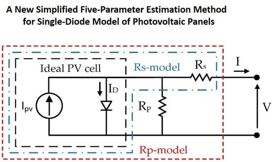
The behavior of PV cells is described by an equivalent circuit model. This model is commonly used to simulate PV cells and is shown in
Figure 1. The advantage of using this model is the integration in the most common electrical software like MATLAB and PSpice environments [
51]. These electric models are integrated to design PV systems as power converters or PV plants.
The cell’s behavior in the absence of solar irradiance is a diode p-n junction, and can be represented by the Shockley equation. The well-known constitutional equation of the diode is as follows:
where
VD is the diode voltage and:
In Equation (2), vt is called the thermal voltage and the terms of the previous equations are defined as:
q is the electron charge (−1.60217646 × 10⁻¹⁹ C)
A is the ideality factor of the diode
k is the Boltzmann’s constant (−1.380653 × 10⁻²³ J/K)
I0 represents the inverse saturation current
T is the temperature (expressed in Kelvin)
The pair of electron-hole is generated due to the photovoltaic effect in the presence of solar irradiance. The charge carriers begin to flow through the external circuit generating the photocurrent
Ipv. Indeed, the photocurrent
Ipv depends on the absorbent capacity of the semiconductor material of the incident irradiance flux [
52,
53,
54]. Inserting the photocurrent in Equation (1) gives the ideal description of the PV cell with a current generator connected in parallel to the diode. The output current of the ideal PV cell is described as follows:
The PV cell actually has some losses caused by the resistance of the connections and the material. The R
s resistor is inserted in the ideal model of the PV cell to consider the losses by introducing the single diode Rs-model. Therefore, the relation of the output current becomes:
The Rs-model in Equation (4) requires four parameter values, i.e., Ipv, I0, A, and Rs.
Although, the Rs-model does not consider the leakage current in the PV cell, making the model inaccurate. To introduce the effect of leakage current, a resistance
Rp is introduced. This model is called the Rp-model, and the output current is determined by the following equation:
In
Figure 1, Expression (3) corresponds to the model enclosed with the black dashed frame, Expression (4) corresponds to the model enclosed with a blue dash-dotted frame and Expression (5) corresponds to the model enclosed with red dashed frame.
The Rp-model introduces an additional parameter
Rp with respect to the Rs-model making it a five-parameters model. In the literature, other models with two diodes or three diodes [
14,
55] have been studied; however, the Rp-model is the most used because it is a good compromise between precision and simplicity [
56].
A photovoltaic panel is made by connecting
N number of cells in series and parallel. Connecting the cells in series increases the voltage while connecting them in parallel increases the output current. A panel with the cells connected in series can be described by Equation (5) by adding to the relation of
vt the number of cells
N as follows:
Rhouma et al. [
57] describe the effect of the variation of the individual parameters of the Rp-model in the I–V characteristic of a photovoltaic panel. In particular, the variation of
Rs and
Rp does not affect the short-circuit current and the open-circuit voltage. However, the variation of
Rp changes the slope in the upper part of the I–V curve of the panel in the region of the short-circuit current. Instead, the variation of
Rs changes the slope in the lower part of the I–V curve in the region of the open-circuit voltage.
3. State of the Art on Methods for Parameter Estimation
The Rp-model of photovoltaic panel requires the calculation of five unknown parameters: IPV, I0, Rs, Rp, and A.
Multiple studies in the literature [
16,
17,
18,
19,
20,
21,
22,
23,
24,
25,
26,
27,
28,
29,
30,
31,
32,
33,
34,
35,
36,
37,
38,
39,
40,
41,
42,
43,
44,
45,
46,
47,
48,
49] present methods to extract these parameters for the single-diode model and Chin et al. [
15] presented a review on existing models. There are many types of methods and they are based on experimental [
16,
20,
35,
37], numerical, and optimization techniques [
17,
18,
19,
22,
23,
24,
25,
26,
27,
28,
29,
30,
31,
32,
33,
34,
36,
38,
39,
40,
41,
42,
43,
44,
47,
49] or combinations of these [
21,
45,
46,
48].
Under open circuit and short circuit conditions,
IPV and
I0 can be analytically calculated.
I0 is negligible in a short circuit condition and
IPV =
ISC can be assumed [
18,
40]. Knowing the value of
IPV, the inverse saturation current
I0 can be derived from the open-circuit condition. However, several studies do not apply these hypotheses for greater accuracy [
21,
39].
A numerical solution is required to estimate the values of
A,
Rs, and
Rp and additional equations are requests usually derived from MPP (Maximum Power Point) or an MPP derivative [
19,
38,
39,
40,
45]. Furthermore, the appropriate initial values must be chosen for a reliable convergence of the method used. The initial value of
Rs can be calculated in the slope of the I–V characteristic in the open-circuit region. Instead,
Rp can be derived from the slope in the short-circuit region as proposed by Adamo et al. and Lo Brano et al. [
16,
17]. Furthermore, for the estimation of
Rs and
Rp, Orioli et al. [
20] proposes a tabulated method.
Vergusa et al. [
22] proposed a scalable PV model with an equation interpreted from a circuit point of view without iterations. However, in this work, several variable resistors and voltage controllers are needed to take into account the environment condition.
The various methods proposed are based only on the data from the datasheet [
39]. For the Lambert W function in the method proposed by Batzelis et al. [
23] a new formula has been introduced. With this formula, it is possible to calculate the parameters through seven steps for the direct calculation.
Other methods used time-varying acceleration coefficients particle swarm optimization (TVACPSO) [
24], the hybrid adaptive Nelder–Mead simplex algorithm based on the eagle strategy [
25], algorithms and adapting control parameters [
27], genetic algorithms to estimate parameters [
28], a chaotic whale optimization algorithm [
29], particle swarm optimization [
30], a multiple learning backtracking search algorithm [
34], and combining translation method [
35].
These methods are computationally burdensome and require calculations while being very accurate. Therefore, a combination of complexity and accuracy is the use of iterative methods for parameter estimation.
Silva et al. [
47] expose the disadvantages of some methods [
40,
41,
43,
44] with respect to their proposed model. Mahmoud’s method [
41] has a problem in neglecting the influence of
Rp or
Rs. Villalva [
40] is accurate near the MPP but may be inaccurate in other regions. The method proposed by Nayak [
43] could remain locked in a local minimum, which does not represent the set of parameters during iterations. The Accarino’s method [
44] has a solution for a more accurate calculation, but in this work is stated that this method is not accurate.
However, Silva’s method optimizes the values of
A and
Rs with an iterative algorithm but calculates
Rp through an equation without subsequent improvement. Instead, the method proposed by Hejri and Mokhtari [
48] is able to estimate the parameters for the initial conditions of the curve-fitting methods [
50], which leads to an increase in complexity and the use of two methods. The proposed method attempts to resolve the limits found in the previous analyzed work. Starting from the Rs-model, the value of
A is optimized to then calculate and estimate
Rs and
Rp passing through the Rp-model.
4. Proposed Five-Parameters Estimation Method
The proposed five-parameters estimation method consists of two steps. The first step regards the estimation of the optimal value of the ideality factor A. In this step, the Rs-model is used, the Rp parameter is neglected, and the Rs value is calculated. Subsequently, with the values of A and Rs obtained from step 1, the value of Rp is extracted in step 2. The algorithm has been tested using Matlab software but can be used on any software or programming environment since it is an iterative algorithm that uses simple equations that are easily solved.
4.1. Step 1: Estimation of A and Rs Parameters
In the first step, the Rs-model is used without considering the
Rp resistance; therefore, Equation (4) is employed. In this equation, there are four variables that are
A,
Ipv,
Rs, and
I0 that need to be derived. First, the equations for calculating
I0 and
Ipv starting from the short circuit and open circuit conditions must be obtained. In the short circuit condition, the output PV current
I is equal to the short circuit current
Isc, and the output voltage
V is zero. Thus, by imposing the short circuit condition with
I =
Isc and
V = 0, Equation (4) becomes:
While imposing the open-circuit condition with
I = 0 and
V =
Voc, Equation (4) becomes:
From (8), the equations to derive the photocurrent
Ipv is the following:
Therefore, the equation to calculate
I0 is found replacing the photocurrent value (9) in (7), and the inverse current of the diode is equal to:
The equation for the resistance
Rs is obtained by imposing that in the maximum power point, the derivative of the power with respect to
V is zero. The power equation is obtained multiplying (4) by the voltage
V. The power is derived with respect to
V, and the resulting equation is as follows:
The resistance
Rs is derived from Equation (11), considering that the relationship is valid for each operating point, including the maximum powerpoint. The equation for calculating
Rs is as follows:
Subsequently by replacing
Ipv and
I0 with Equations (9) and (10), the final expression of
Rs is:
The equations found for calculating
I0,
Ipv, and
Rs make the system indeterminate. Indeed, there are three equations with four unknowns, and the ideality factor of diode
A which can take values between 1 and 2 [
21] must be derived. Iteration cycles are used to estimate
A by comparing the value of the voltage at the maximum power point with that given by the manufacturer. Variation of
A has an effect on the thermal voltage
vt, and therefore, on resistance
Rs. Furthermore, the variation of
Rs affects the slope of the I–V characteristic of the panel in part near the open-circuit voltage, as explained in
Section 2.
Considering the current-voltage relation at the maximum power point using Equation (4) and replacing
V =
Vmp and
I =
Imp the maximum power voltage can, thus be obtained:
The proposed algorithm for step 1 is shown in
Figure 2.
The proposed algorithm provides the initial definition of the parameter A imposed equal to 1, the maximum acceptable tolerance for the maximum estimated voltage of 0.1 V, and a maximum finite number of iterations equal to 10,000. Subsequently, the values of vt and Rs are calculated with A = 1 and start with iterations. The value of A is increased by 0.01 if the new calculated maximum voltage is less than the theoretical one; otherwise, it is decreased by 0.01. With the new value of A, I0 is recalculated using (10), Ipv via (9), and Vmp through (14). The algorithm continues until the error is lower than the tolerance set, or the maximum iteration limit is exceeded. Finally, the new value of Rs is recalculated with the new estimated value of A.
4.2. Step 2: Estimation of Rp Parameters
Unfortunately, the Rs-model is not accurate, and the maximum power point found with the new values of
A and
Rs does not match with that reported by the manufacturer. For this reason, the
Rp resistance is introduced using the Rp-model with Equation (5). The procedure is the same as in step 1 with iterations, but this time, the iterated parameter is
Rp. Since the variation of
Rp affects the part of the characteristic I–V near the short-circuit current, the comparison will be made on the maximum power current. The proposed method provides an initial estimation of
Rp that can be obtained from the relation of the maximum power as follows:
From (15),
Rp is extracted which is worth:
For the first
Rp estimation, the
Ipv and
I0 values used are those originating from the Rs-model and, therefore, from the Equations (9) and (10). However, in the iterations of the proposed algorithm, they must be derived from the relation (5) of the complete model of
Rp. Using the short circuit and open circuit voltage conditions, the new values of
I0 and
Ipv will be:
The algorithm for calculating
Rp with the proposed method is shown in
Figure 3.
As explained above, in step 2 of the proposed method it is necessary to have an initial estimation of the value of the resistance
Rp. Taking the values of
Rs,
A, and
Ipv of the model
Rs coming out of step 1,
Rp is calculated using Equation (16). The iterative algorithm involves the initial definition of the number of iterations and the maximum accepted tolerance. The number of iterations equal to 10,000 and tolerance equal to 0.001 A are chosen. The new values of
I0 and
Ipv are calculated with the initial value of
Rp expected for the Rp-model using the Equations (17) and (18). The method involves obtaining the current in the conditions of maximum power in Equation (5) with
V =
Vmp. The maximum power obtained is compared with that given by the manufacturer, and the
Rp is changed. If the current is less than the expected value,
Rp is increased by 0.1 ×
itI; otherwise, it is decreased by 0.1 ×
itI. The error between the maximum calculated and expect current is compared with the maximum acceptable tolerance. This procedure is repeated a number of times until the error is as low as then the expected tolerance or when the maximum number of iterations is reached. The root of nonlinear function fzero() in MatLab is used to calculate the maximum current [
58].
4.3. Electrical Variation Model and Error Metric
The equations describing a PV panel must consider the variation in temperature and solar irradiance. The datasheets of the manufacturers give the data of voltage and current in the various conditions: short-circuit, open-circuit, and maximum power. Furthermore, the manufacturers give the values of the open-circuit voltage temperature coefficient (
Kv) and the short-circuit current temperature coefficient (
Ki). The coefficients
Kv and
Ki, expressed as %/°C for both or V/°C and A/°C, respectively, considering variations in voltage and current with respect to temperature. The series resistance remains unchanged with temperature and solar irradiance variations [
15]. The most simple method is constant parameter modeling, working under the hypothesis that
IPV and
I0 are affected by the environmental conditions, while two parameters indicted with
Rs, and
Rp, are considered constant. However, this approximation is too idealistic.
Instead, the parallel resistance
Rp can be considered dependent only on the variation of solar irradiance [
15] according to the following relation:
where
Rp,STC is the parallel resistance calculated in the proposed method in the standard test conditions,
GSTC is the standard solar irradiance that is 1000 W/m
2, and G is the new solar irradiance. The thermal voltage
vt depends only and exclusively on the temperature through Equation (6).
Silva [
47] proposed an equation for
Rs which takes into account its relationship with temperature and solar irradiance variation as follows:
where
B is the exponential solar irradiance coefficient, and
kR represents the linear temperature coefficient. These coefficients are obtained in an iterative way by comparing the experimental curves present in the datasheet of the panel under examination.
Instead, the short-circuit current has a strong dependence on irradiance and little on the variable temperature through the
Ki coefficient. The new simplified short circuit current relation is as follows:
where
Ki is the reduction coefficient of the current based on the temperature expressed in A/°C, and
TSTC is the temperature in the standard test conditions, which is 25 °C.
The open-circuit voltage has a low variation with solar irradiance, but it changes a lot with the temperature according to the
Kv coefficient given by the manufacturer. The new
VOC relation dependent on the temperature and solar irradiance is as follows:
In order to evaluate the accuracy of the model, the root-mean-square error (
RMSE) as an error metric is used [
59]. The
RMSE is calculated on the PV current and normalized (
NRMSE) respect to the expected current as follows:
where
IS,i is the output simulation value,
IM,i is the expected value and
n is the number of values.
5. Results and discussion
The proposed estimation method has been implemented in Matlab environment using a single diode Equation (5). A multi-crystalline PV module KC200GT from Kyocera [
60], with 54 cells connected in series, was chosen to test the method. The parameters provided by the manufacturer in the STC used in the proposed method are shown in
Table 1.
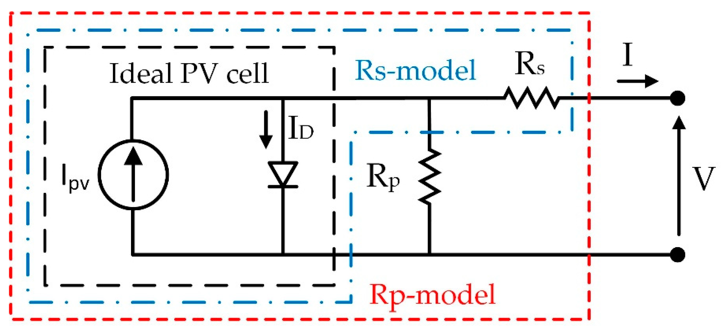
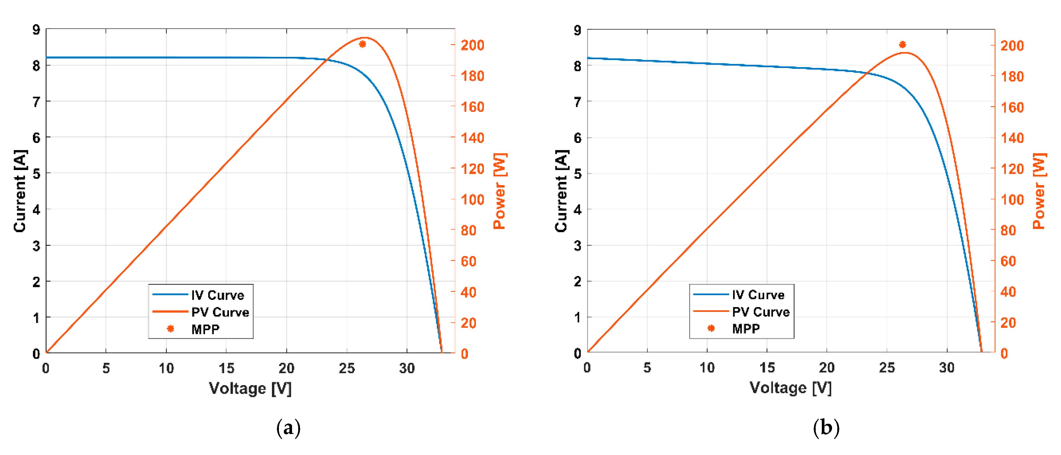
Figure 4 shows the graph of the various phases of the output data of the proposed method for the KC200GT panel. The second step shown in
Figure 4c, the maximum power point coincides with the expected one. Indeed, the addition and variation of shunt resistance
Rp change the I–V curve in the area near the short-circuit current.
In order to simulate the behavior of the panel with a model described by Equation (5) as a function of temperature and solar irradiance variations, (19), (21), and (22) are used. These equations have been chosen, but other models [
15] can be considered.
Figure 5 shows the trends of the I–V curve with respect to variations in solar irradiance (
Figure 5a) and temperature (
Figure 5b) for the KC200GT panel. The solar irradiance and temperature values were chosen based on those reported on the panel’s datasheet.
In order to validate the proposed method, the experimental data provided by datasheets are used. Nevertheless, the I–V curves in the datasheet are not in a tabular format, and data must be extracted. Therefore, using the tools available in [
61], the curves are digitalized and transferred on a spreadsheet. However, the data extracted from the curves are different from those declared in the tables of the datasheet because these values have a declared tolerance. To get a more accurate estimation of the parameters, the newly extracted data of the I–V curve in STC from the datasheet’s image is used.
The proposed method is tested both with datasheet values and curves.
Table 2 shows the comparison results of some examined works and the proposed method. The parameter values of [
40,
41,
43,
44] were taken by [
47], which were extracted from the datasheet curves. In [
48], there are two types of parameters extracted: from the STC values of the datasheet and extracted by the curve fitting method. The
RMSE and
NRMSE are calculated for each method to evaluate de accuracy.
As can be seen, the proposed method presents the best results for the RMSE and NRMSE among the compared methods in STC. The RMSE and NRMSE have values of 0.07 A and 0.87 %, respectively.
Figure 6 shows the comparison between the expected and manufacturer I–V curves at different values of solar irradiance and temperature. The curves in STC almost overlap, but in different conditions around the maximum power point, the I–V curves present displacements. Indeed, this is due to the choice of the model for the environmental variations of the I–V characteristic.
Furthermore,
NRSME is calculated for different operating conditions. The results are shown in
Table 3, where
NRMSEAv is the average of all the errors in different operating conditions of the specific method.
From the previous table, the proposed method with the values derived from the datasheet table shows the lowest error. Indeed, even if for solar irradiance of 400 W/m
2 and 200 W/m
2, it has a greater error than [
40], and [
43], the average error is the lowest of the examined methods.
To reduce the error, the equation proposed by [
47] is used, which takes into account the variation of
Rs with respect to the operating conditions. The
kR and
B values of the KC200GT panel extracted from datasheet’s curves provided in [
47] are equal to 0.1 and 0.77, respectively.
The new curves extracted using [
47] with the KC200GT datasheet curves input data are shown in
Figure 7. The curves are extracted at various solar irradiance and temperature values, and they are compared with those of the datasheet.
With this model, the error is reduced, and there is a better approximation of the estimated curve that tends to the expected curve of the datasheet.
Table 4 shows the
NRMSE and the average of the examined methods and of the proposed. In this case, the proposed method, which uses the I–V datasheet curves, has the lowest error for all solar irradiance values compared to the result of the model without Equation (20). The error on the temperature variation is not the best of all, but the average error is the lowest and is equal to 1.28%.
Figure 8 shows the normalized error pattern for all the examined methods for different solar irradiance values. It should be noticed how the method proposed on the curves of the datasheet (black line) presents the best error with the descriptive model used on the panel.
Figure 9 shows the bar chart of the average error on the variations of solar irradiance and temperatures of all the examined methods.
The proposed method presents excellent results in STC compared to the examined methods. Indeed, in the STC conditions, the single-diode Rp-model for the extraction of the I–V and P–V characteristics is normally used. However, to have accurate I–V and P–V characteristics that approach the expected values, an appropriate model must be used. Indeed, the average error
NRMSE of the proposed method is decreased by 41% with the use of the equation proposed by [
47].


