3.3.1. Daily Clearness Coefficient Estimates
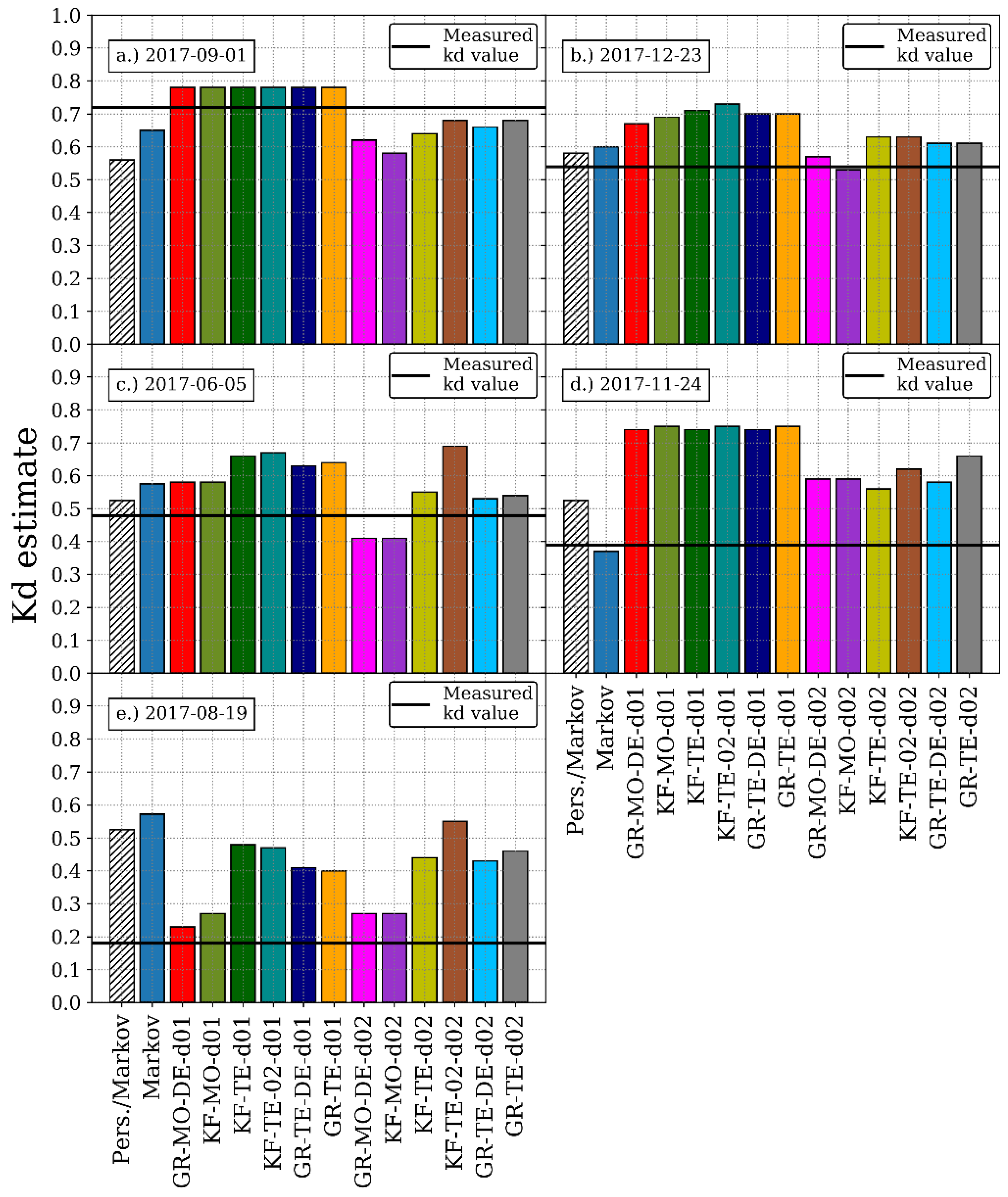
Figure 9 shows, for each of the considered days, the estimates of the daily clearness coefficient (
) obtained with each of the considered models (i.e., the first part of the proposed Markov model, persistence model, and the WRF experiments).
Figure 9 presents these estimates as bar plots, with each bar representing a different model and its height representing the corresponding estimated value of
. The black horizontal lines in each of these panels indicates the corresponding
measured values. The blue bars in
Figure 9 correspond to the mean
values estimated by the proposed Markov model, for each day.
For 1 September 2017 (
Figure 9a), all WRF experiments overestimated the daily clearness coefficient for the outer domain and underestimated it for the inner domain. The persistence model underestimated the
by
and the propose Markov model underestimated the
by
.
Figure 9b,c show the case of 23 December 2017and 5 June 2017respectively. For these cases, the Markov model and the Persistence model overestimated the measured
values, although the Persistence model had smaller overestimation than the proposed Markov model. For 23 December 2017 (
Figure 9b), the KF-MO experiment for the inner domain estimated the
with an error of 0.01, being the closest estimate to the real
. In the case of 5th June 2017, only the KF-MO and GR-MO-DE experiments, both for the inner domain, underestimated the daily clearness coefficient,
. In the rest of the cases the
was overestimated.
Figure 9d corresponds to the case of 24th November 2017. This day presented a case where local-scale events seem to be responsible for the high extinction values over the incoming GHI. For this day, the Markov model shows a better performance than the Persistence model at estimating the
. In this case the
of the proposed Markov model is
, while the persistence model exhibited a
. For this day, the WRF experiments also overestimated the measured daily clearness coefficient,
consistently. Since the Markov model has a better performance at estimating transitions that are frequently found in the variable records used to train it, it is possible to assume that the events corresponding to the high levels of cloudiness for 24 November 2017, are events that frequently occurred during the March 2016–February 2017 period.
Figure 9e shows the simulations for 19 August 2017. This day, in contrast with 24 November 2017, was a case characterized by the presence of a synoptic scale event over the Caribbean Sea. Although all experiments reproduce high levels of GHI extinction at the location of the event, the GHI series reproduced over Medellín greatly vary from experiment to experiment. As can be seen from
Figure 9e, the
estimates corresponding to GR-MO-DE-d01 and KF-MO-d01 are those closest to the measured value, with the GR-MO-DE-d01 estimate having the lowest error of 0.05. For this day, the Markov model reproduced an average
of 0.58 and the persistence model an average
of 0.53, which are values that lie far from the observed value of 0.18. This indicates that this type of events, which are not so commonly observed over the study region and are caused by events that occur beyond local scales, are hardly captured by the Markov model.
In general, the Markov model and the persistence model showed a similar performance at estimating the , except for 1 September 2017 and 24 November 2017, were the propose Markov model had a better performance. It is also noted that, in general, the WRF experiments for the inner domain tended to produce lower estimates than their counterpart in the outer domain.
Additionally, although the proposed Markov
estimates presented in
Figure 9 are averaged values and the distribution of the estimates is not shown, we must indicate that the Markov model is only capable of producing 2 to 3 different states for each day presented in
Figure 9.
3.3.2. Hourly Estimates of GHI
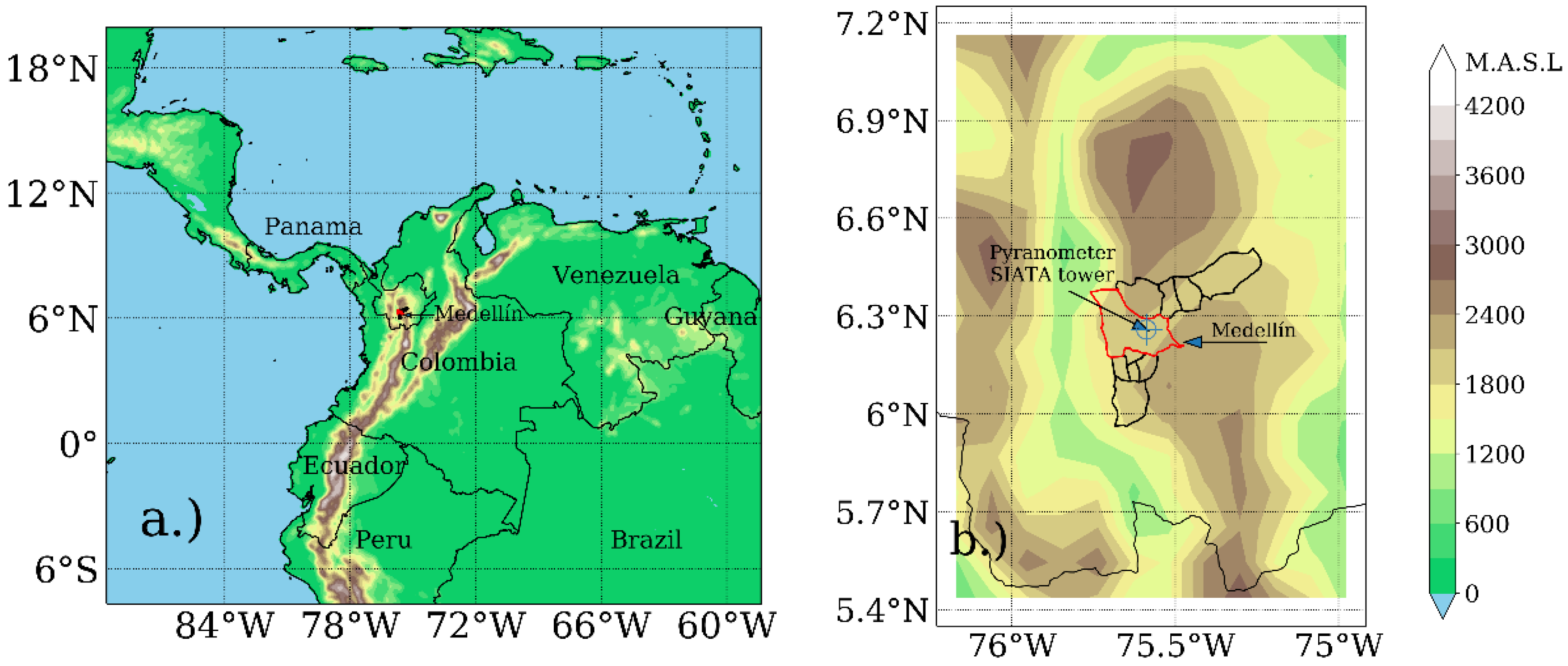
We evaluated the skill of the WRF model and the proposed Markov model at simulating the GHI at Medellín, Colombia, for 5 non-consecutive days with different cloud cover conditions (
Table 2). Although only 5 simulation days do not represent a comprehensive simulation period, the comparison between the proposed Markov model and the WRF model at estimating the GHI for these 5 days still represents a good indicator of the performance of the proposed Markov model. The chosen days were selected based on their daily clearness coefficient value. For each particular day, we ran six simulations of the WRF model with different combinations of microphysics and cumulus schemes (
Table 3). These simulations were later compared against the simulations obtained with the Markov model for the same 5 days.
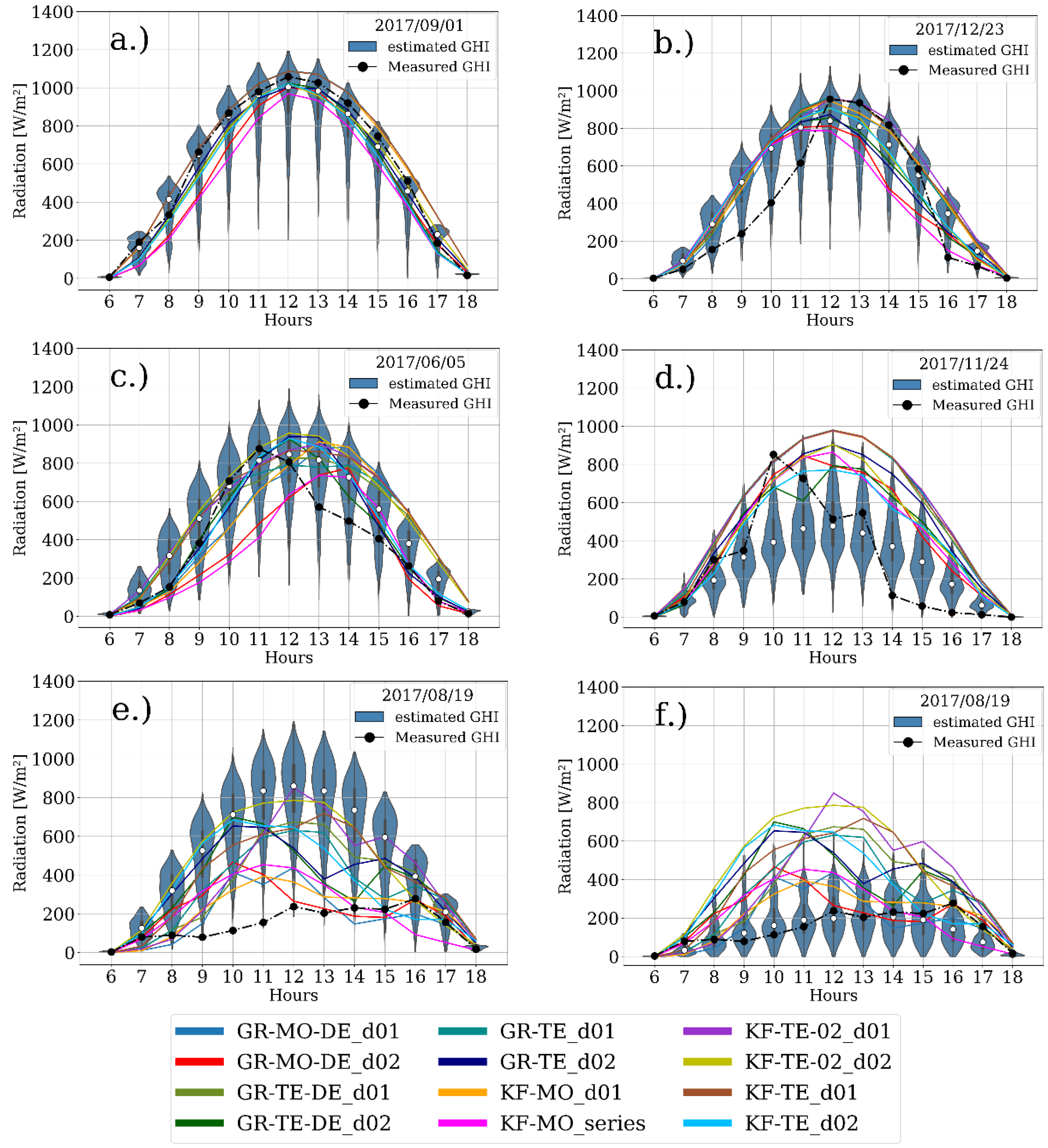
Since the Markov model produces estimates in a stochastic way, each simulation results in a different hourly series of GHI, meaning that several realizations of a single day could be obtained in order to observe the overall behavior of the proposed Markov model. For this reason, and noting that the model is computationally inexpensive, each day in
Table 2 is simulated 1000 times using the proposed Markov model. The resulting series for each day are plotted as violin plots, which are discriminated by each hour of the day, and are presented along with the estimate GHI series obtained with the WRF experiments in
Figure 10. Violin plots are useful in this case because they include the approximate probability distribution of the estimates and also have information about the statistical metrics of the distribution such as the interquartile range and the median of the series. As in
Figure 6, the white dots in the violin plots indicate the median value of the distributions and the height of the boxes inside each violin plot indicates the position and magnitude of the IQR of each distribution calculated as the difference between the Q3 and Q1 values, respectively.
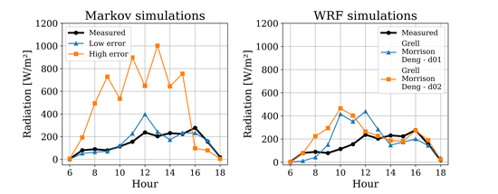
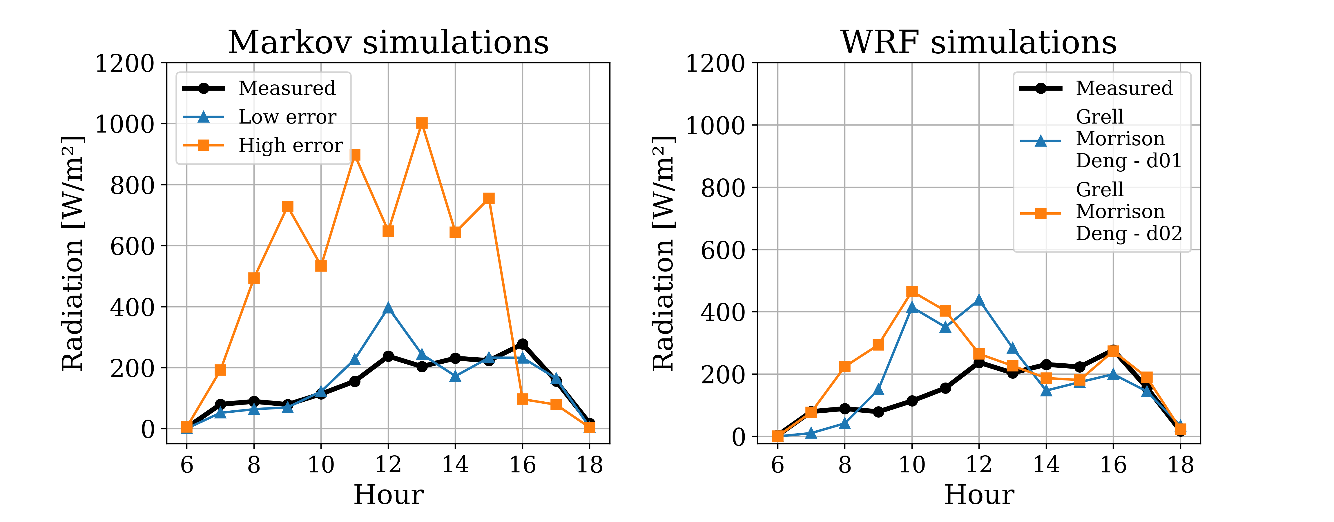
Figure 10 presents the GHI hourly simulations obtained with the Markov model and the WRF model for each of the 5 selected days. The blue distributions correspond to the violin plots of the Markov estimates for each hour of each day and the colored lines correspond to the WRF GHI series for each experiment and for each domain considered (i.e., outer domain, d01 and inner domain, d02). The dashed black lines correspond to the measured hourly series of GHI for each day.
Figure 10a presents the hourly distributions of GHI for a clear sky day (1 September 2017,
). For this day, the measured values of GHI are close to the IQR of the Markov estimate distributions. In the case of the WRF estimates, it is observed that series have a similar shape to the measured series, with the estimates of the KF-MO experiment presenting an RMSE increase of 77 W/m
2 from the outer domain (d01) with respect the inner domain (d02). In the case of the inner domain, d02, the WRF estimates consistently underestimated the measured GHI series.
Figure 10b presents the estimates for 23 December 2017. For this day, the measured series presented higher atmospheric extinction values during the morning hours than during the evening hours. For this day, the Markov model mostly overestimated the GHI during the morning hours, with only some extreme estimates falling near the measured values. This behavior is similar to that exhibited by most of the WRF experiments for this day. During the first evening hours (i.e., 12LT–15LT), the Markov model produced GHI values that were, in general, closer to the measured GHI values than the estimates produced by the WRF series for the inner domain (d02). In the case of the WRF estimates for the outer domain (d01), WRF produced GHI values that were very similar to the measured values and to the median values of the Markov distributions. During the last evening hours (i.e., 16LT–18LT), both models consistently overestimated the measured GHI values.
In the case of 5 June 2017 (
Figure 10c), the Markov model had a satisfactory performance at estimating the GHI values between 9 LT–12 LT. However, it mostly overestimated the GHI during the afternoon hours as the measured values are near the lower tails of the estimate distributions. This matches the behavior of most of the WRF experiments, which also overestimated the GHI during the evening hours. However, the WRF experiments that used the Thompson and Eidhammer scheme, for the inner domain (i.e., KF-TE-d02, GR-TE-d02 and GR-TE-DE-d02), underestimated the clearness coefficient during the morning hours, unlike the rest of the experiments.
For the case of 24 November 2017 (
Figure 10d), the Markov model consistently forecasted
states that were closer to the measured
, which caused the hourly GHI estimates of the Markov model to be closer to the hourly measured GHI values than the estimates obtained with the WRF experiments. This can be corroborated in
Figure 9d. Although the Markov model had a better performance at estimating the hourly GHI than the WRF experiments for this day, both models consistently overestimated the measured GHI values for most of the evening hours (i.e., 14LT–18LT).
The 19 August 2017 (
Figure 10e) exhibits the lowest daily clearness coefficient value among the simulated days (
). As it was previously mentioned, the high levels of cloudiness observed on this day are mainly associated to a tropical depression crossing the Caribbean and that would later transform into Hurricane Harvey [
67]. For this day, the Markov model consistently overestimated the
for each of 1000 simulations performed (
Figure 9e). These overestimations lead to an incorrect selection of the hourly MTM, which in turn, causes the consistent overestimations of the hourly values of GHI. This case is an example of how the estimates of the first part of the model largely affect the performance of the second part of the model. For this day, some of the WRF experiments exhibited a better performance at estimating the GHI than the Markov model. This was the case of the experiments that considered Morrison as the microphysics scheme. It was also observed that the outer domain (d01) estimates showed a better agreement with the measured GHI values than the nested domain (d02) estimates. Given that for 19 August 2017, the first part of the Markov model is not able to correctly simulate the measured state of the
in any of the 1000 simulations, an extra set of 1000 simulations were performed to observe the behavior of the second part of the model alone (i.e., the simulation of the hourly GHI). In order to do this, for these extra set of simulations, the state of
used as input for the second part of the Markov model was forced to be equal to the measured value (i.e.,
). The simulations obtained in this way for the Markov model are presented in
Figure 10f. Most of the measured values of the GHI now fall inside the IQR of the Markov estimate distributions. In this case, when the base state of the series, which can be represented by the
, is correctly estimated, the model frequently reproduces GHI values that are closer to the measurements than in the opposite case (
Figure 10e).
In order to assess the general performance of the Markov model at estimating the hourly GHI for the 5 selected days,
Table 6 presents the summary of the RMSE errors of the hourly estimates of GHI obtained with the Markov model for each of the simulated days. The last row of
Table 6 corresponds to the case where the estimated
was set equal to the measured
. The RMSE values presented for the Markov model correspond to the median values of the RMSE distributions.
Table 6 also shows the summary of the RMSE errors of the hourly estimates of GHI obtained with the GR-MO-DE experiment since it has one of the highest performances at estimating the hourly GHI. The RMSE values presented for this experiment correspond to the mean value between the RMSE error for the outer domain, d01 and the inner domain, d02. Additionally, the RMSE median value of the persistence-Markov model is also presented in order to provide further benchmarking for the proposed Markov model.
According to
Table 6, for 1st September 2017, the Markov model exhibits an RMSE error of 144 W/m
2, which is lower than the RMSE value for the Persistence-Markov model but higher than the mean RMSE produced by the WRF experiment. This indicates a lower performance at estimating the hourly GHI for this day compared to the WRF experiment but an improvement with respect the persistence-based model. For 23 December 2017, the Markov model, the persistence-Markov model and the WRF experiments presented a similar performance at estimating the hourly GHI, all of them exhibiting nRMSE values of 47%, 45% and 46%, respectively. For the case of 6 June 2017, the performance of the Markov model increases with respect to the performance of the WRF experiments at estimating the GHI, however, the persistence-Markov model presents an improvement with respect the proposed Markov model. For the case of 24 November 2017, it can be seen that the proposed Markov model has a better performance than the persistence-Markov mode and the WRF model, presenting a lower RMSE than the other two models. This shows that for this particular day, neither the persistence-based model nor the WRF model were capable of simulating the correct state of the
, while the proposed Markov model did. Finally, for the case of 19 August 2017, the WRF presents a better performance at reproducing the effects of the larger scale event over the region of study, while the proposed Markov model and the persistence-Markov model fail to reproduce these effects over the GHI and thus, result in estimations with high RMSE values.
In general, the Markov model exhibits a lower RMSE values at estimating the hourly GHI in Medellín than the WRF experiment except for 1 September 2017 and 19 August 2017. For the latter simulation day, the Markov model is not able to reproduce the effects of the large-scale event over the region of study, while the WRF experiment GR-MO-DE is capable of producing large atmospheric extinction levels over the hourly GHI estimates.
As an additional assessment of the performance of these models for the 5 days selected,
Table 7 shows the median of the RMSE values corresponding to each model. It can be observed that the proposed Markov model had a better performance at estimating the GHI than the persistence-Markov model. Also, it can be seen that the WRF model had a similar performance to the proposed Markov model with a small improvement of 3 W/m
2.


