Article

Assessing Evidence for Weather Regimes Governing Solar Power Generation in Kuwait

National Center for Atmospheric Research, Boulder, CO 80307, USA
*
Author to whom correspondence should be addressed.
Energies 2019, 12(23), 4409; https://doi.org/10.3390/en12234409
Submission received: 19 October 2019 / Revised: 14 November 2019 / Accepted: 15 November 2019 / Published: 20 November 2019
(This article belongs to the Special Issue Applications of Artificial Intelligence in Renewable Energy)

Abstract

:
With electricity representing around 20% of the global energy demand, and increasing support for renewable sources of electricity, there is also an escalating need to improve solar forecasts to support power management. While considerable research has been directed to statistical methods to improve solar power forecasting, few have employed finite mixture distributions. A statistically-objective classification of the overall sky condition may lead to improved forecasts. Combining information from the synoptic driving conditions for daily variability with local processes controlling subdaily fluctuations could assist with forecast validation and enhancement where few observations are available. Gaussian mixture models provide a statistical learning approach to automatically identify prevalent sky conditions (clear, semi-cloudy, and cloudy) and explore associated weather patterns. Here a first stage in the development of such a model is presented: examining whether there is sufficient information in the large-scale environment to identify days with clear, semi-cloudy, or cloudy conditions. A three-component Gaussian distribution is developed that reproduces the observed multimodal peaks in sky clearness indices, and their temporal distribution. Posterior probabilities from the fitted mixture distributions are used to identify periods of clear, partially-cloudy, and cloudy skies. Composites of low-level (850 hPa) humidity and winds for each of the mixture components reveal three patterns associated with the typical synoptic conditions governing the sky clarity, and hence, potential solar power.

1. Introduction

Improving forecasts of power from solar panels, whether short-range forecasts out to a few hours, or longer, such as subseasonal forecasts, has been the subject of much research in recent years (as reviewed by [1,2,3,4]). The target uses of the forecasts include planning future installations, optimizing plant operations and efficiency, or balancing load demand and delivery [5]. As outlined by [6], the choice of forecasting technique varies with the decision and time-scale of interest (hourly, daily, and multiday). Solar power can be estimated as a function of solar irradiance, the solar photovoltaic cell properties, and temperature (e.g., [7,8]), allowing power forecasts to leverage weather forecasting of sky conditions. While statistical techniques are often favored for very short-term modeling, satellite-based forecasts of cloud advection perform well in the multihour range [9,10], and longer-term forecasts are generally found to be most reliable from numerical weather prediction models (e.g., WRF Solar [11]).
A thorough review of the common forecast approaches at different time aggregations is provided by [4], finding that almost 75% of methods are statistics based. Of these, deterministic irradiance forecasts often combine clustering analyses to classify the sky state [12,13,14,15], followed by a machine-based learning algorithm to develop forecasts [16,17,18,19]. However, clustering analyses are subjective and can result in model overfitting [20]. Approaches that combine clustering with machine learning can challenge the principle of parsimonious modelling by requiring additional estimation to achieve accurate forecasts [21].
The statistical technique of finite mixture distributions is often used with success for wind power forecasts (e.g., [5,22,23,24]), but seldom employed for solar power [25]. Finite mixture distributions and their companion hidden Markov models (HMMs) [26] are fully probabilistic models representing the full distribution of event frequencies, where HMMs also incorporate a transition probability for the shift between each regime. This option is attractive, as the atmospheric regimes driving clear or cloudy sky conditions cannot necessarily be known a priori [27]. HMMs have been used to good effect in combination with atmospheric patterns to improve climate projections [28] and seasonal forecasts (e.g., [29]). However, the drawback of HMMs is that if the state transition matrix is unconstrained, an infinite number of distribution components and state transitions can be identified [30]. As this is inefficient and often difficult to interpret [31], a simpler approach is to identify the likely candidates in the absence of transitions, i.e., to use finite mixture models to develop a plausible hypothesis of driving mechanisms.
To date, finite mixture models have tended to employ Dirichlet multinomial distributions on prepartition, subhourly data to forecast solar irradiance from sky clearness indices [20,32]. A drawback of the Dirichlet method is the assumption that sky clarity is adequately described by a discrete distribution, yet the continuous nature of sky clarity can render it sensitive to the choice of data bins [33]. While there is considerable evidence for multimodality in the continuous distributions of solar irradiance indices [21,34,35], the use of other statistical distributions has seldom been explored. HMM and other Markov chain processes have similarly focused on subhourly to subdaily forecasts [16,18,19,36]. However, the transition matrices between sky states are often assumed to be the same for all days, once seasonality has been removed, which is unlikely to be correct [37] and can lead to substantial forecast errors [38,39].
We suggest that a better forecast may be achievable by combining knowledge of both daily and subdaily solar irradiance fluctuations to allow for both the synoptic driving conditions for daily variability, and microscale processes, e.g., governing convective cloud development [40]. As a first step in this analysis, we employ finite mixture models to explore whether it is possible to identify clear, overcast, or cloudy days and associated synoptic processes in an objective manner. Mesoscale variability could then be incorporated in a nonhomogeneous HMM to dictate the subhourly evolution of irradiance, dependent on the daily state (e.g., [36,38,41]). This paper presents the first part of that analysis for a large solar power plant in the western desert area of Kuwait where the Shagaya Renewable Energy Plant is being deployed. The statistical model is applied to daily values of sky clearness indices. Composites of geopotential mean relative humidity and wind at 850 hPa are then produced for the representative days of each distribution component to identify driving synoptic conditions.
Section 2 summarizes the data and methods used for this research, and Section 3 presents initial exploratory analyses. The results of the mixture model development and relation to geopotential humidity and winds are presented in Section 4, while Section 5 concludes and suggests further research avenues.

2. Data and Methods

2.1. Data

We combine on-site observations with other ground-based meteorological observations for the exploratory analysis, and satellite observations of global horizontal irradiance (GHI) for statistical analyses.
Meteorological data from surface weather stations and meteorological towers were supplied by the Kuwait Institute for Scientific Research (KISR) and their contractors for the period July 2012 to June 2018, with approximately 20% missing data. Supplementary daily observations were obtained from three Global Historical Climatological Network Daily (GHCND) stations [42,43] in addition to hourly observations from eleven Integrated Surface Data locations [44]. All ground-based observation stations are indicated in Figure 1, together with the site of interest. The meteorological data were used for the exploratory analyses presented in Section 3, to establish likely mechanisms affecting sky clarity.
HelioSat-4 [45] is a physical model that uses aerosol properties, total column water vapor, and ozone content from the Copernicus Atmospheric Monitoring Service (CAMS) in combination with Meteosat satellite observations of cloud properties to derive the global, direct, and diffuse solar surface irradiances, at ground level and normal angle of incidence. McClear [46] provides estimates of the Global Horizontal Irradiance (GHI) under cloudless (or clear-sky) conditions, and has been validated for 1-min measurements. McCloud [45] uses the McClear model to estimate the GHI under all sky conditions by calculating the reduction in irradiance caused by clouds. Time-series are available for a given location from 2004 to the present in 1 min, 15 min, 1 h, 1 day, and 1 month sums over Europe, Africa, the Middle East, the Atlantic Ocean, and eastern parts of South America, interpolated to the point of interest [46]. The data used for the present study are for complete years 2005–2017, 1 min interval GHI (McClear and McCloud) at the Shagaya Renewable Energy Plant, available from the Copernicus portal (http://atmosphere.copernicus.eu/).
Daily mean 850 hPa wind vectors and 850 hPa relative humidity fields for the greater Middle East area were obtained from the ERA-Interim reanalysis archive [47] for the period 2005–2017.

2.2. Method

2.2.1. Clearness Index

Clouds present the greatest source of subhourly variability in GHI, with the fractional changes greatest at midday [2,17]. Furthermore, daily and seasonal changes in the zenith angle can introduce other errors in GHI measurements [38]. While solar power forecasts are usually at a high temporal resolution (e.g., [1]), this analysis is on daily, and longer, variability. Given that our focus is on synoptic-scale conditions, we avoid the influence of daily zenith angle fluctuations (i.e., sunrise and sunset) and very short irradiance fluctuations by working with cumulative daily total GHI for the purpose of this initial assessment. Further, cumulative daily total GHI removes the emphasis of diurnal variability, or the errors inherent in utilizing the mean of highly variable data. Seasonal variations in the theoretical available irradiance are removed by working with the Clearness Index.
The Clearness Index ( K t ) [48] is the quotient of observed surface ( I t ) and extra-terrestrial irradiation (Itclr), or K t = I t I t c l r . This nondimensional measure is also deseasonalized, and can be calculated for any temporal aggregation from hourly to monthly (e.g., [49]). K t values are in the range (0, 1), where values of 0 correspond with dark or fully obscured skies, and values of 1 correspond to the theoretical maximum sky clarity for that particular location, time, and date.

2.2.2. Mixture Distributions

Finite mixture models are selected to account for the unobserved heterogeneity caused by different sky conditions; a benefit is that exact proportions of the mixes do not need to be defined, but rather, can be inferred from the data [26]. We assume that the data can be described by a homogeneous mixture (i.e., >1 components derived from the same distribution family) for the different sky conditions. Further, we assume that the data are continuously distributed and are Gaussian derived [13,21], although some have suggested that other distributions are more appropriate [36].
An independent mixture model f ( y ) with k components is the weighted average, w i , for i = 1 ,   ,   k component distributions with θ the parameter space, f i ( y ; θ i ) and for w i 0 . Where:
f ( y ) = i = 1 k w i f i ( y ; θ i )
and
i = 1 k w i = 1
The mean is a weighted average of the component means, while the variance comprises the weighted variance of each component distribution and an increase in dispersion arising from the difference in component means. Differences in the means tending to zero, or a vector of component weights tending to (0, 1), is indicative of the underlying data converging to a single component distribution [50]. For a two-component distribution, i = 1 ,   2 , the mean, μ , and variance, σ , of the mixture can be expressed as:
μ = w 1 μ 1 + w 2 μ 2
σ 2 = w 2 σ 1 2 + w 2 σ 2 2 + w 1 w 2 ( μ 1 μ 2 ) 2
While it is possible that a two-component distribution may exist with a small difference between the means and different estimates of variance, manifesting as a unimodal mixture, it is unlikely in this case where there are clear differences in the sky conditions.
The Expectation-Maximization (EM) algorithm [51] is an iterative, two-step procedure to estimate the partition ( w i ) between distinct distributions and the relevant parameters ( θ i ), when the exact values for w i and θ i are unknown. The Expectation step (E-step) develops an “averaged” log-likelihood function for the parameter estimates, which is then maximized to select improved parameter estimates in the Maximization step (M-step). The process is iterated until convergence is reached for estimates of w i and θ i [52]. Other algorithms such as the Levenburg-Marquardt or Quasi-Newton methods may be more efficient and effective in avoiding “noninteresting maxima”, but they are far more sensitive to the initial parameter estimates [22].
The selection of the initial parameter estimates can be important to ensure that convergence to a global optimum is achieved. However, where maxima that are not representative of the data, or insignificant differences between distributions occur, the process is repeated with different initial conditions to validate the result. We adopt the default conditions for initial parameter estimates, convergence (changes in loglikelihood   1   ×   10 8 ), and iterations (<1000) provided in the R software package (version 3.5.2, R Core Team, Vienna, Austria) [53], mixtools [54]. That is, data are randomly partitioned into k components with parameters selected as the initial mean of each component and a common variance. Mixture weights are random selections from a uniform distribution (i.e., random selections that are normalized to sum to 1). The optimum number of distribution components is tested using a combination of Akaike’s Information Criterion (AIC) [55] and a bootstrapping approach with 100 repetitions.

3. Exploratory Evidence

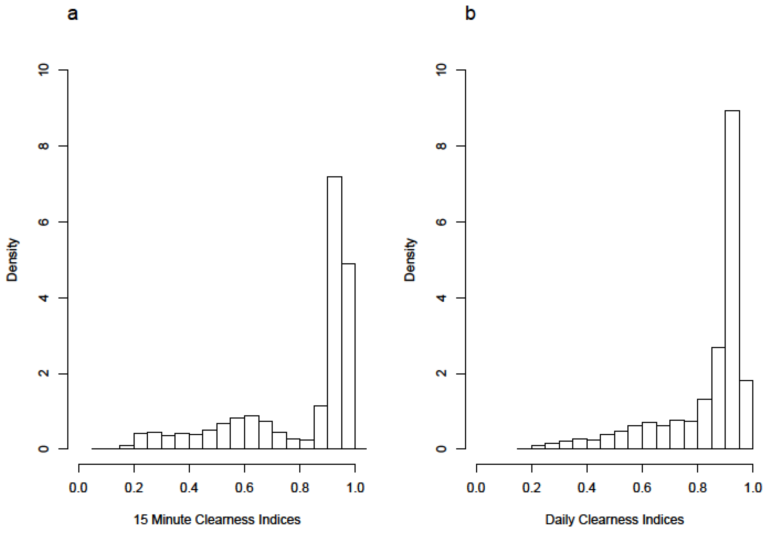
The annual distributions of the daily and subdaily clearness index (in Figure 2) demonstrate multimodal properties that are suggestive of multiple component distributions. This multimodality is more apparent for subdaily (Figure 2a) than daily data (Figure 2b). However, the subdaily data includes twilight observations at zenith angles <10° that may cause abnormal fluctuations of irradiance [56].
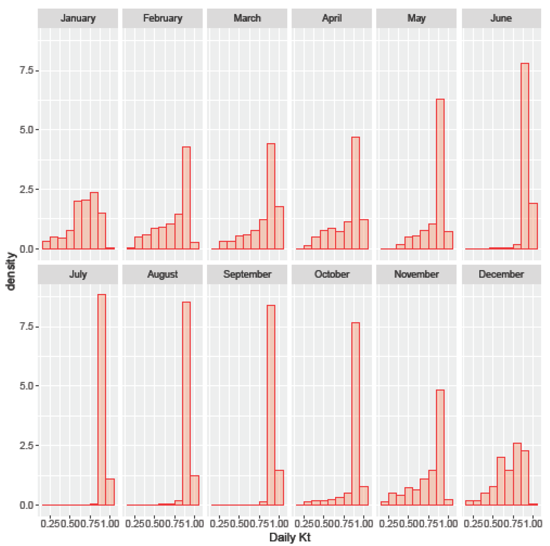
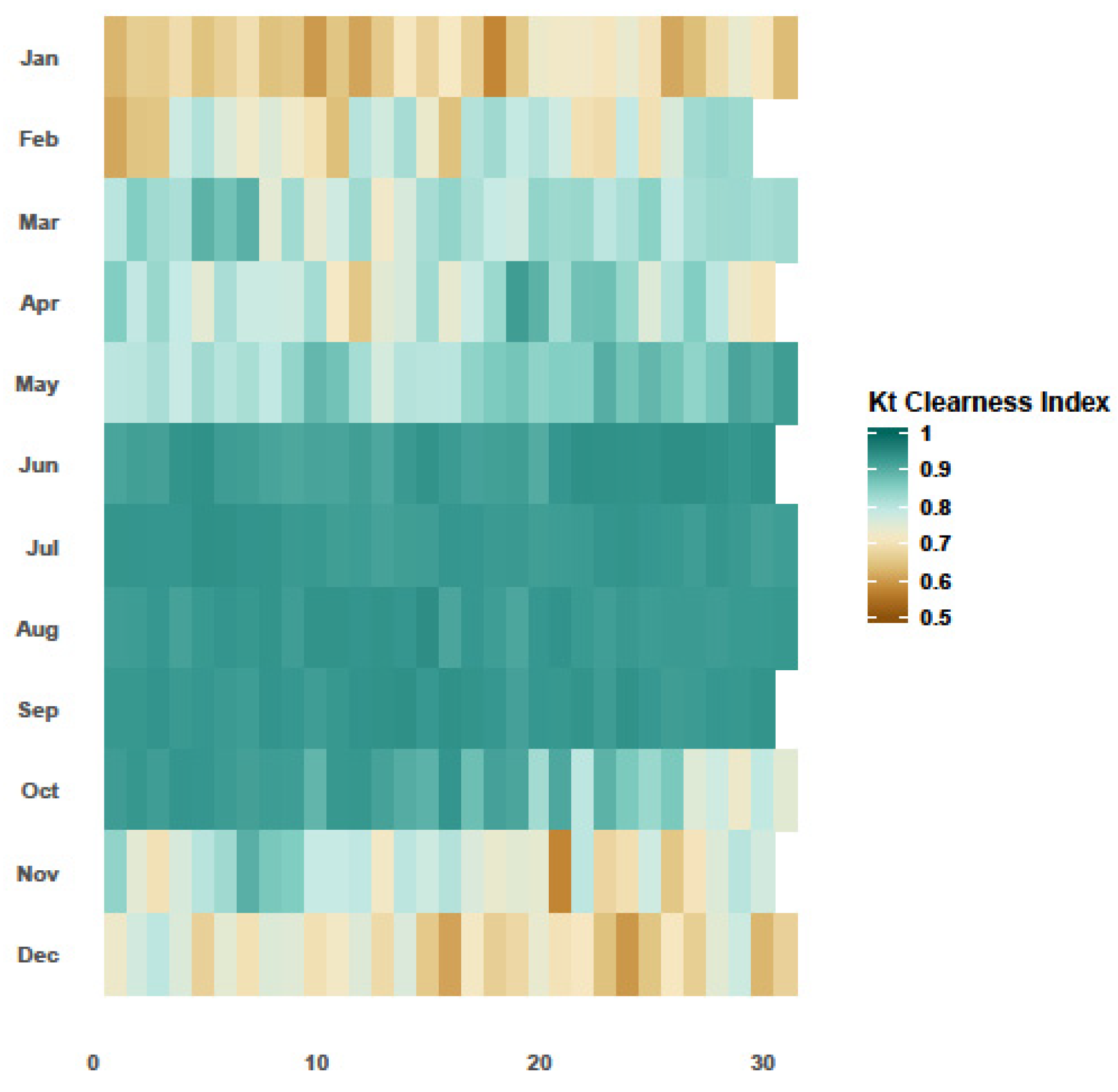
Plotting the daily data by month (Figure 3) suggests that the same component distributions are more prevalent at different times of the year, reflecting seasonal weather fluctuations at the site, and the influence of latitude on solar intensity. For instance, Ref. [57] noted that winter season precipitation is useful for estimating the likely frequency of dust-storms, which would correlate with periods of lower sky clarity as appears to be the case for January, February, and December. Ref. [58] identified that poor visibility events in the UAE arise either as a result of dry, wind-induced dust storms, or wetter weather such as fog or haze. Thus, rare poor visibility events during the summer are probably related to the Haboob winds transporting dust from the east and northeast [59]. Stronger wind speeds occur the hotter months, strengthening in response to the Low Level Jet during nocturnal hours and offset from the peak GHI [60]. In contrast, the winter north and northwesterly winds bringing higher relative humidity from the Gulf of Aman impact at-site visibility while more stable, clearer, conditions occur in the summer [59], as is apparent in Figure 3 and Figure 4.
Figure 4 illustrates the daily clearness index, calculated from a time series of extra-terrestrial and received solar irradiation between 2005 and 2017. For each day, the color represents the mean value of the clearness index on that calendar day. While the figure is for illustrative purposes only, it highlights the fact that for the majority of the year there are excellent visibility conditions ( K t x > 0.8 ), with the lowest values occurring during the winter months.
As daily maximum temperatures at the Shagaya Renewable Energy site were only available since 2012, GHCND Abraq Mazraa observations of daily maximum temperature are used as a proxy to increase the period of record for comparison with daily clearness. The correlation between daily maximum temperatures and daily clearness values is plotted in Figure 5 for 2007–2017. This supports the correlation between the highest daily temperatures and the highest values of clearness also found by [59]. Again, this result reflects the local climatology and expected seasonal pattern of higher temperatures during July and August, as well as the highest clearness values during the summer months (darker shades of red).
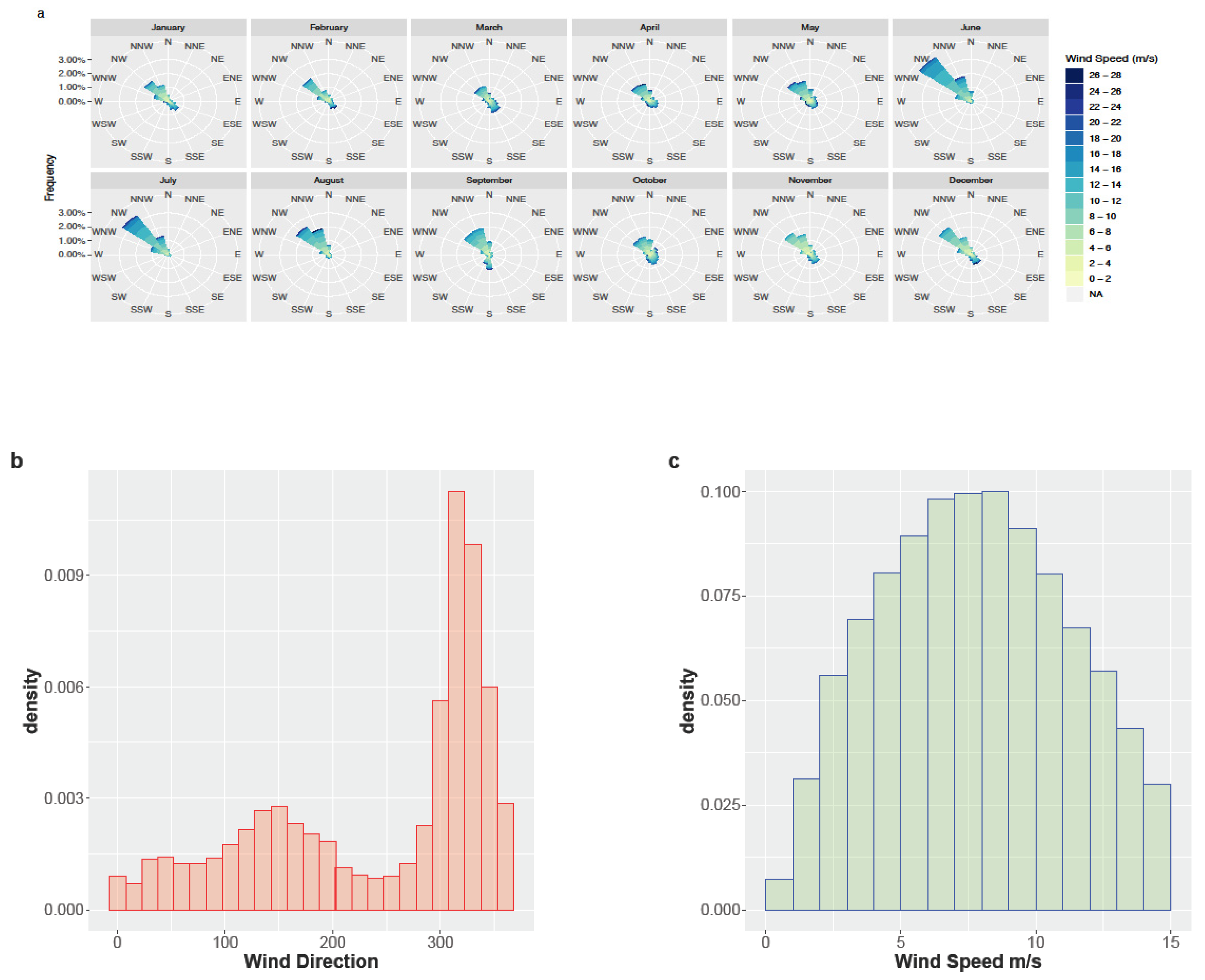
Solar panel efficiency starts to reduce at high temperatures, similar to the reduced efficiency of wind power at high wind speeds. Recent research has demonstrated that while higher winds and temperatures (and, thus, sky clarity) are seasonally coincident, higher wind speeds occur nocturnally, allowing for more consistent power generation at sites combining wind and solar generation [60]; refer to Figure 6a. The higher wind speeds can occasionally lead to dust storms that will impair solar panel productivity [58], but these events are rare.

4. Results

We assume that the distribution of daily clearness indices is Gaussian distributed. From the evidence presented in Section 3, we expect a minimum mixture of two Gaussians, representing good and poor conditions. A disadvantage of mixture model distributions is that they can appear to improve statistical model fitting by using multiple mixture components to fit the data, rather than each component truly arising from a different driving regime. With this in mind, it is possible that the data are derived from a single exponential-type distribution [36]. Alternative distribution families, including gamma, exponential, and Weibull, were compared using a range of model diagnostics (loglikelihoods, AIC, goodness of fit), for distributions with 1 to 5 components (not shown), concluding that multiple Gaussian distributions are the most appropriate choice [61].

4.1. Mixture Models

The exploratory analyses suggest that the multiple components of a distribution arise from seasonally varying processes, and that within each season, there is not as much variability as there is annually. Therefore, we can test the validity of model assumption using a bootstrapping approach, iterating the model fits for 100 random samples of the data.
Figure 7 illustrates loglikelihood values for mixture distributions with 1 to 5 components fitted to daily clearness indices; the process was repeated for 100 data samples, with no replacement. The continued increase in loglikelihood values could suggest that there are 4 or 5 processes represented by the mixture components. However, closer inspection reveals that the increase in loglikelihood from 3 to 4, and then 4 to 5, is not significant. Further, the fourth and fifth components have very low mixture weights and parameters that overlap with another distribution component, indicating that a three-component Gaussian mixture model is the optimum configuration.
The final 3-component mixture model is illustrated in Figure 8a in red, together with the results from 100 random samples in darker red. Figure 8b shows the improvement in data representation by comparing the quantile–quantile plots of a single distribution (grey), the three components (red), and three components from 100 random samples (darker red). The mixture model comprises:
Component   1   :   μ 1 =   0.61 σ 1 = 0.16 w 1 = 0.27
Component   2   :   μ 2 = 0.89 σ 2 = 0.05 w 2 = 0.17
Component   3   :   μ 3 = 0.93 σ 3 = 0.02 w 3 = 0.56
where μ i is the component mean; σ i is the component standard deviation; and w i is the component weight. Thus, the resultant probability density function for the full mixture has μ = 0.83 and σ = 0.06 .
We then examine the fitted distributions for plausibility to ensure that they reflect the assumption of seasonality where each component arises from a common set of processes. Posterior probabilities from the fitted mixture distributions are used to identify periods of clear, partly-cloudy, and cloudy skies. When plotted with respect to the calendar day, the hypothesis that the three components reflect seasonal weather patterns is supported. Figure 9 illustrates the observed value of daily clearness by month in purple; gray dots represent the mean of each distribution component with respect to the associated posterior probability of each observation. Thus, there are gaps in Component 1′s sequence of gray dots during July and August when the sky clarity is highest. The posterior probabilities predict that daily clearness indices fall mainly into Component 3; purple dots are spread around two components, but are largely concentrated in the top portion of the chart. In contrast, the posterior probabilities and observed indices for January and December show a broader spread across all values, with a higher concentration of values in Component 1.

4.2. Identification of Synoptic Weather Conditions

Statistical testing (Figure 7) indicates that a three-component Gaussian mixture model best represents the distribution of daily clearness indices for this site in Kuwait. However, it is important to evaluate whether there is a physical mechanism underlying the data distribution, or if the apparent mixture components arose as a statistical artefact of the data. [31] assessed the reality of distribution components by comparing the posterior probabilities to geopotential heights. We use the posterior probabilities to select the days that have an observed clearness index closest to the component mean. While the components are not calculated seasonally, the selected dates naturally partition according to summer, winter, and spring/fall seasons. We then composite the low-level (850 hPa) relative humidity and low-level (850 hPa) winds on those days to examine whether there is a clear signal of large-scale synoptic behavior (Figure 10). This elevation was selected as an appropriate elevation to minimize the influence of the variable terrain, while still illustrating surface weather patterns through the strength and direction of moisture fluxes. As with [31], allowing the data to self-organize into regimes has led to more readily-interpretable weather patterns (explained below).
Higher relative humidity can lead to aerosol particle growth and coalescence, reducing visibility [58]. This is apparent in Component 1 (35–40% humidity), where the anticyclonic pattern centered over Oman results in moderate south-westerly flow over Kuwait transporting moist air from the Red Sea. Component 2 has the lowest relative humidity; however, the strong northwesterly winds bring dust from the desert regions of Iraq (25–30% humidity). Component 2 also has a pronounced trough centered over the Persian Gulf, associated with warmer conditions and the potential for strong thunderstorms [62]. The high pressure center in Component 3 is over Saudi Arabia, resulting in dry and light westerly winds over Kuwait that are more favorable for calm, clear conditions.
Several authors have examined weather and circulation patterns over the Arabian Peninsula [57,62,63,64], with particular emphasis on improved water resource management and renewable energy production. Differing seasonal foci mean that there are differences between the low-level wind and relative humidity patterns found here and the defined weather types, as well as differences between the studies in question. For instance, [64] focused solely on dust outbreaks throughout the year, while [65] examined dust outbreaks only during the wet season. [66] did not specifically identify weather types; however, they sought to explain their mixture distribution allocations with regard to typical surface wind regimes in the United Arab Emirates.
Ref. [63] characterized weather types over Saudi Arabia using the Lamb weather-type classification [67], finding that days with a cyclonic pattern followed by those with southeast directional flow are the most frequent during the summer. This behavior parallels Component 3, where the high pressure center is over Saudi Arabia, and is the most frequently occurring pattern during the summer months. It also is the component that describes the clearest days (i.e., K t > 0.9 ), as it is associated with the synoptic patterns generating less moisture and dust transport.
All three components appear to correspond with anticyclonic weather patterns described by [62], with high pressure centers over Iran or Saudi Arabia and lower pressure centers over north Africa. Ref. [64] confirm that a trough over the Arabian Peninsula advects dust and is most commonly associated with the onset of the Arabian Peninsula summer low during March to June. During summer months, this same pattern is recognized as the summer Shamal, causing the majority of dust storms during this season [58,64]. Ref. [65] confirm that the processes generating dust storms are very different in winter and summer, with the majority of dust storms arising during the spring and early summer. Further, winter months are affected by the southerly shift of the polar jet, increasing the contrast in north and south air masses over the Arabian Peninsula, bringing more frontal systems and poorer visibility. Again, this finding supports the frequency and occurrence of Component 1 during the winter and transition seasons.

5. Discussion and Conclusions

As support for renewable sources of electricity goes up [68], increasing the number of solar power installations, there is also an increasing need to improve solar power forecasts. Recent private–public–academic research identified the need to combine nowcasts of solar power forecasts at high temporal resolution (subhourly), with coarser temporal resolution forecasts (out to several days) to meet decision-maker needs [1]. The research presented here contributes to longer duration forecasts by identifying large-scale weather systems affecting sky clarity and reducing reliance on computationally-intensive numerical weather predictions.
Many have examined the use of statistical methods to improve solar forecasting, but limited attention has been paid to the use of finite mixture distributions. Often, those applications utilizing finite mixture models have employed Dirichlet multinomial distributions on prepartitioned, subdaily data [20,32], and neglected the influence of larger-scale processes on the subdaily fluctuations. Apart from the drawback of selecting an appropriate bin interval to describe continuous data with discrete distributions, we consider that an objective classification of the overall sky condition is more likely to lead to improved forecasts.
We examined daily clearness indices for the Shagaya renewable energy plant in Kuwait, calculated from satellite retrieved global horizontal irradiance data between 2005–2017. After analyzing the data, we assume that they are best described by a mixture of Gaussian distributions [13,21]. Exploratory analysis reveals that there are multiple peaks in the data frequency, and that the variability in subdaily clearness indices is greater than in daily clearness indices. As noted by [40], subdaily variability is more sensitive to local features and meso- to micro-scale processes, while multiday variability is dependent on synoptic-scale systems. Our focus here was on the synoptic-scale, and so we analyzed only the distribution of daily indices.
Seasonal distribution of the clearness indices corresponded with the observed weather conditions. That is, the hottest periods of the year, which have low humidity and stable air conditions, also had the highest clearness indices, while the lowest values correspond with the more turbulent conditions of winter and the transition seasons. A three-component Gaussian mixture model fit these data very well, with the posterior probabilities reproducing the observed distribution of clearness indices throughout the year. Alternative distribution families were examined and found to be inadequate, highlighting instead that multiple mixture components can erroneously improve the statistical model in the absence of physical reasoning. Utilizing the posterior probabilities, we composited the 850 mb humidity and 850 mb wind on the day’s most clearly assigned to each component. This procedure generated three patterns associated with the typical synoptic conditions governing the sky clarity, and hence, potential solar power.
As noted by several authors, limited attention has been paid to circulation types, specifically with respect to precipitation occurrence, over the Arabian Peninsula [58,63,65]. The sparse observation network is frequently cited as the cause for the low research interest in this region. Thus, Kuwait’s lower density observation network has received even less attention than larger neighboring countries such as Iran or Saudi Arabia. While our focus was not directly on precipitation occurrence, it is correlated with cloudy sky conditions. Poor visibility conditions also arise from haze, fog, or dust storms [58], which can also be attributed to wind conditions generated by different circulation types. We have not determined specific weather types, but the exploratory analyses of wind and temperatures throughout the year generally corroborate the circulation patterns and associated air flow directions. The peak wind gusts occur during the summer months, with much lower wind speeds during the transition seasons and winter. This result emphasizes that poor visibility conditions are driven by different mechanisms during the summer and winter [63,65], where cooler temperatures are likely to give rise to more fog and cloud cover rather than the dust storms of the summer.
The similarities that are apparent between the humidity and geopotential wind patterns for each distribution component and the weather type studies, as well as the differences between each of these studies, suggest that a hidden Markov Model would be appropriate for statistical forecasting. This approach would permit the data to identify the hidden states driving sky clearness, rather than predefining the process from a short observation time series. Further developments of such a model should focus on incorporating the subdaily variability to create a stochastic weather generator dependent on the hidden large-scale synoptic processes together with local microscale drivers. For instance, [31] found some success in predicting subdaily wind two to five days out using hidden Markov Models. A key requirement for developing such a model would be sufficiently long observation series to estimate the transition probabilities for each weather pattern.

Author Contributions

Conceptualization, M.R.T. and S.E.H.; methodology, M.R.T and E.G..; formal analysis, M.R.T.; writing—original draft preparation, M.R.T.; writing—review and editing, M.R.T., S.E.H., E.G., C.K., T.J.; visualization, M.R.T.; supervision, E.G.; project administration, S.E.H.; funding acquisition, S.E.H.

Funding

The National Center for Atmospheric Research is sponsored by the National Science Foundation (NSF). Support for this work was provided by a grant from the Kuwait Institute for Scientific Research.

Acknowledgments

Data were obtained from the NCAR Data Repository, NOAA’s Global Historical Climate Network, and the Copernicus Atmosphere Monitoring Service. Thanks to Abby Jaye for assistance in producing Figure 10; to James Done for providing comments on a draft version of the manuscript; and to Barbara Brown for useful statistical insights. All calculations were carried out in R (http://www.r-project.org/), using packages tidyverse, mixtools and cowplot.

Conflicts of Interest

The authors declare no conflict of interest. The funders had no role in the design of the study; in the collection, analyses, or interpretation of data; in the writing of the manuscript, or in the decision to publish the results.

References

  1. Haupt, S.E.; Kosovic, B.; Jensen, T.; Lazo, J.; Lee, J.; Jimenz, P.; Cowie, J.; Wiener, G.; McCandless, T.; Rogers, M.; et al. Building the Sun4Cast system: Improvements in solar power forecasting. Bull. Am. Meteorol. Soc. 2018, 121–135. [Google Scholar] [CrossRef]
  2. Lohmann, G. Irradiance variability quantification and small-scale averaging in space and time: A short review. Atmosphere 2018, 9, 264. [Google Scholar] [CrossRef]
  3. Reikard, G.; Haupt, S.E.; Jensen, T. Forecasting ground-level irradiance over short horizons: Meteorological and time series models. Renew. Energy 2017, 112, 474–485. [Google Scholar] [CrossRef]
  4. Van der Meer, D.W.; Widén, J.; Munkhammar, J. Review on probabilistic forecasting of photovoltaic power production and electricity consumption. Renew. Sustain. Energy Rev. 2018, 81, 1484. [Google Scholar] [CrossRef]
  5. Bracale, A.; De Falco, P. An advanced bayesian method for short-term probabilistic forecasting of the generation of wind power. Energies 2015, 8, 10293–10314. [Google Scholar] [CrossRef]
  6. Diagne, M.; David, M.; Lauret, P.; Boland, J.; Schmutz, N. Review of solar irradiance forecasting methods and a proposition for small-scale insular grids. Renew. Sustain. Energy Rev. 2013, 27, 65–76. [Google Scholar] [CrossRef]
  7. Clack, C.T.M. Modeling solar irradiance and solar pv power output to create a resource assessment using linear multiple multivariate regression. J. Appl. Meteorol. Climatol. 2017, 56, 109–125. [Google Scholar] [CrossRef]
  8. Deshmukh, M.K.; Deshmukh, S.S. Modeling of hybrid renewable energy systems. Renew. Sustain. Energy Rev. 2008, 12, 235–249. [Google Scholar] [CrossRef]
  9. Auligné, T. Multivariate minimum residual method for cloud retrieval. Part I: Theoretical aspects and simulated observations experiments. Mon. Weather Rev. 2014. [Google Scholar] [CrossRef]
  10. Auligné, T. Multivariate minimum residual method for cloud retrieval. Part II: Real observations experiments. Mon. Weather Rev. 2014. [Google Scholar] [CrossRef]
  11. Jimenez, P.A.; Hacker, J.P.; Dudhia, J.; Haupt, S.E.; Ruiz-Arias, J.A.; Gueymard, C.A.; Deng, A. WRF-Solar: Description and clear-sky assessment of an augmented NWP model for solar power prediction. Bull. Am. Meteorol. Soc. 2016, 97, 1249. [Google Scholar] [CrossRef]
  12. Greybush, S.J.; Haupt, S.E.; Young, G.S. The regime dependence of optimally weighted ensemble model consensus forecasts of surface temperature. Weather Forecast. 2008, 23, 1146. [Google Scholar] [CrossRef]
  13. Lai, C.S.; Jia, Y.; McCulloch, M.D.; Xu, Z. Daily clearness index profiles cluster analysis for photovoltaic system. IEEE Trans. Ind. Inf. 2017, 13, 2322. [Google Scholar] [CrossRef]
  14. Lorenz, E.; Hammer, A. Short term forecasting of solar radiation based on satellite data. In Proceedings of the EUROSUN2004, Freiburg, Germany, 20–23 June 2004. [Google Scholar]
  15. Mellit, A.; Massi Pavan, A.; Lughi, V. Short-Term forecasting of power production in a large-scale photovoltaic plant. Sol. Energy 2014, 105, 401–413. [Google Scholar] [CrossRef]
  16. Hocaoglu, F.O.; Serttas, F. A novel hybrid (Mycielski-Markov) model for hourly solar radiation forecasting. Renew. Energy 2017, 108, 635–643. [Google Scholar] [CrossRef]
  17. McCandless, T.C.; Haupt, S.E.; Young, G.S. A regime-dependent artificial neural network technique for short-range solar irradiance forecasting. Renew. Energy 2016, 89, 351–359. [Google Scholar] [CrossRef]
  18. Morf, H. Sunshine and cloud cover prediction based on Markov processes. Sol. Energy 2014, 110, 615–626. [Google Scholar] [CrossRef]
  19. Poggi, P.; Notton, G.; Muselli, M.; Louche, A. Stochastic study of hourly total solar radiation in Corsica using a Markov model. Int. J. Climatol. 2000, 20, 1843–1860. [Google Scholar] [CrossRef]
  20. Frimane, Â.; Aggour, M.; Ouhammou, B.; Bahmad, L. A Dirichlet-multinomial mixture model-based approach for daily solar radiation classification. Sol. Energy 2018, 171, 31–39. [Google Scholar] [CrossRef]
  21. Munkhammar, J.; Widén, J. A Markov-chain probability distribution mixture approach to the clear-sky index. Sol. Energy 2018, 170, 174–183. [Google Scholar] [CrossRef]
  22. Ailliot, P.; Monbet, V. Markov-Switching autoregressive models for wind time series. Environ. Modell. Softw. 2012, 30, 92–101. [Google Scholar] [CrossRef]
  23. Carta, J.A.; Ramírez, P. Use of finite mixture distribution models in the analysis of wind energy in the Canarian Archipelago. Energy Convers. Manag. 2007, 48, 281–291. [Google Scholar] [CrossRef]
  24. Zhang, J.; Chowdhury, S.; Messac, A.; Castillo, L. A Multivariate and multimodal wind distribution model. Renew. Energy 2013, 51, 436–447. [Google Scholar] [CrossRef]
  25. Inman, R.H.; Pedro, H.T.C.; Coimbra, C.F.M. Solar forecasting methods for renewable energy integration. Prog. Energy Combust. Sci. 2013, 39, 535–576. [Google Scholar] [CrossRef]
  26. Zucchini, W.; MacDonald, I.L. Hidden Markov Models for Time Series: An Introduction Using R; CRC Press: Boca Raton, FL, USA, 2009. [Google Scholar]
  27. Hughes, J.P.; Guttorp, P. A class of stochastic models for relating synoptic atmospheric patterns to regional hydrologic phenomena. Water Resour. Res. 1994. [Google Scholar] [CrossRef]
  28. Bellone, E.; Hughes, J.P.; Guttorp, P. A hidden Markov model for downscaling synoptic atmospheric patterns to precipitation amounts. Clim. Res. 2000, 4415, 15. [Google Scholar] [CrossRef]
  29. Carey-Smith, T.; Sansom, J.; Thomson, P. A hidden seasonal switching model for multisite daily rainfall. Water Resour. Res. 2014, 50, 257–272. [Google Scholar] [CrossRef]
  30. Ghahramani, Z. An introduction to hidden models and bayesian networks. Int. J. Pattern Recognit. Artif. Intell. 2001, 15, 9–42. [Google Scholar] [CrossRef]
  31. Bessac, J.; Ailliot, P.; Cattiaux, J.; Monbet, V. Comparison of hidden and observed regime-switching autoregressive models for (u, v)-components of wind fields in the northeastern Atlantic. Adv. Stat. Climatol. Meteorol. Oceanogr. 2016, 2, 1–16. [Google Scholar] [CrossRef]
  32. Soubdhan, T.; Emilion, R.; Calif, R. Classification of daily solar radiation distributions using a mixture of Dirichlet distributions. Sol. Energy 2009, 83, 1056. [Google Scholar] [CrossRef]
  33. Béranger, B.; Duong, T.; Perkins-Kirkpatrick, S.E.; Sisson, S.A. Tail density estimation for exploratory data analysis using kernel methods. J. Nonparametric Stat. 2019, 31, 144–174. [Google Scholar] [CrossRef]
  34. Fernández-Peruchena, C.M.; Bernardos, A. A comparison of one-minute probability density distributions of global horizontal solar irradiance conditioned to the optical air mass and hourly averages in different climate zones. Sol. Energy 2015, 112, 425–436. [Google Scholar] [CrossRef]
  35. Jurado, M.; Caridad, J.M.; Ruiz, V. Statistical distribution of the clearness index with radiation data integrated over five minute intervals. Sol. Energy 1995, 55, 469–473. [Google Scholar] [CrossRef]
  36. Tabone, M.D.; Callaway, D.S. Modeling variability and uncertainty of photovoltaic generation: A hidden state spatial statistical approach. IEEE Trans. Power Syst. 2015, 30, 2965. [Google Scholar] [CrossRef]
  37. Ngoko, B.O.; Sugihara, H.; Funaki, T. Synthetic generation of high temporal resolution solar radiation data using Markov models. Sol. Energy 2014, 103, 160–170. [Google Scholar] [CrossRef]
  38. Alimohammadi, S.; He, D. Multi-Stage algorithm for uncertainty analysis of solar power forecasting. In Proceedings of the 2016 IEEE Power Energy Society General Meeting (PESGM), Boston, MA, USA, 17–21 July 2016; pp. 1–5. [Google Scholar] [CrossRef]
  39. Köhler, C.; Steiner, A.; Saint-Drenan, Y.-M.; Ernst, D.; Bergmann-Dick, A.; Zirkelbach, M.; Ritter, B. Critical weather situations for renewable energies—Part B: Low stratus risk for solar power. Renew. Energy 2017, 101, 794–803. [Google Scholar] [CrossRef]
  40. Rodríguez-Benítez, F.J.; Arbizu-Barrena, C.; Santos-Alamillos, F.J.; Tovar-Pescador, J.; Pozo-Vázquez, D. Analysis of the intra-day solar resource variability in the Iberian Peninsula. Sol. Energy 2018, 171, 374–387. [Google Scholar] [CrossRef]
  41. Ailliot, P.; Bessac, J.; Monbet, V.; Pène, F. Non-Homogeneous hidden Markov-switching models for wind time series. J. Stat. Plann. Inference 2015, 160, 75–88. [Google Scholar] [CrossRef] [Green Version]
  42. Menne, M.J.; Durre, I.; Korzeniewski, B.; McNeal, S.; Thomas, K.; Yin, X.; Houston, T.G. Global Historical Climatology Network—Daily (GHCN-Daily), Version 3.24; NOAA National Climatic Data Center: Asheville, NC, USA, 2018. [Google Scholar] [CrossRef]
  43. Menne, M.J.; Durre, I.; Vose, R.S.; Gleason, B.E.; Houston, T.G. An Overview of the Global Historical Climatology Network-Daily Database. J. Atmos. Ocean. Technol. 2012, 29, 897–910. [Google Scholar] [CrossRef]
  44. NOAA NCEI CDO. Integrated Surface Data, DS3505, NOAA National Centers for Environmental Information Climate Data Online. Available online: www.cdo.NCEI.noaa.gov (accessed on 18 April 2018).
  45. Qu, Z.; Oumbe, A.; Blanc, P.; Espinar, B.; Gesell, G.; Gschwind, B.; Wald, L. Fast radiative transfer parameterisation for assessing the surface solar irradiance: The Heliosat-4 method. Meteorologische Zeitschrift 2017, 26, 33–57. [Google Scholar] [CrossRef]
  46. Lefèvre, M.; Oumbe, A.; Blanc, P.; Espinar, B.; Gschwind, B.; Qu, Z.; Morcrette, J.-J. McClear: A new model estimating downwelling solar radiation at ground level in clear-sky conditions. Atmos. Meas. Tech. 2013, 6, 2403. [Google Scholar] [CrossRef] [Green Version]
  47. Dee, D.P.; Uppala, S.M.; Simmons, A.J.; Berrisford, P.; Poli, P.; Kobayashi, S.; Vitart, F. The ERA-Interim reanalysis: Configuration and performance of the data assimilation system. Quart. J. Roy. Meteorol. Soc. 2011, 137, 553–597. [Google Scholar] [CrossRef]
  48. Liu, B.Y.H.; Jordan, R.C. The interrelationship and characteristic distribution of direct 2418, diffuse and total solar radiation. Sol. Energy 1960, 4, 1–19. [Google Scholar] [CrossRef]
  49. Nemes, C.; Ciobanu, R.; Rugina, C. Probabilistic analysis of Sky clearness index for solar energy systems planning. In Proceedings of the 2018 Smart City Symposium Prague (SCSP), Prague, Czech Republic, 24–25 May 2018; pp. 1–9. [Google Scholar] [CrossRef]
  50. Wilks, D.S. Statistical Methods in the Atmospheric Sciences, 3rd ed.; Academic Press Inc.: Waltham, MA, USA, 2011. [Google Scholar]
  51. Dempster, A.P.; Laird, N.M.; Rubin, D.B. Maximum likelihood from incomplete data via the EM algorithm. J. Roy. Stat. Soc. Ser. B Methodol. 1977, 39, 1–38. [Google Scholar]
  52. Do, C.B.; Batzoglou, S. What is the expectation maximization algorithm? Nat. Biotechnol. 2008, 26, 897–899. [Google Scholar] [CrossRef] [PubMed]
  53. R Core Team. A Language and Environment for Statistical Computing. R Foundation for Statistical Computing: Vienna, Austria, 2018. Available online: http://www.r-project.org/ (accessed on 28 December 2018).
  54. Benaglia, T.; Chauveau, D.; Hunter, D.R.; Young, D. Mixtools: An R package for analyzing finite mixture models. J. Stat. Softw. 2009, 32, 1–29. [Google Scholar] [CrossRef] [Green Version]
  55. Akaike, H. A new look at the statistical model identification. IEEE Trans. Autom. Control 1974, 19, 716–723. [Google Scholar] [CrossRef]
  56. Hinkelman, L.M.; Schaeffer, N. Relating solar resource and its variability to weather and climate across the northwestern United States. Sol. Energy 2017, 157, 966–978. [Google Scholar] [CrossRef]
  57. Nasrallah, H.A.; Balling, R.C.; Selover, N.J.; Vose, R.S. Development of a seasonal forecast model for Kuwait winter precipitation. J. Arid Environ. 2001, 48, 233–242. [Google Scholar] [CrossRef]
  58. Aldababseh, A.; Temimi, M. Analysis of the long-term variability of poor visibility events in the UAE and the link with climate dynamics. Atmosphere 2017, 8, 242. [Google Scholar] [CrossRef] [Green Version]
  59. Naizghi, M.S.; Ouarda, T.B.M.J. Teleconnections and analysis of long-term wind speed variability in the UAE. Int. J. Climatol. 2017, 37, 230–248. [Google Scholar] [CrossRef]
  60. Naegele, S.M.; McCandless, T.C.; Greybush, S.J.; Young, G.S.; Haupt, S.E.; Al-Rasheedi, M. Climatology of wind variability for the Kuwait Region. Renew. Energy 2019, in press. [Google Scholar]
  61. Peyvandi, S.; Amirshahi, S.H.; Hernández-Andrés, J.; Nieves, J.L.; Romero, J. Spectral recovery of outdoor illumination by an extension of the Bayesian inverse approach to the Gaussian mixture model. J. Opt. Soc. Am. A 2012, 29. [Google Scholar] [CrossRef] [PubMed]
  62. Almazroui, M.; Dambul, R.; Islam, M.N.; Jones, P.D. Atmospheric circulation patterns in the Arab region and its relationships with Saudi Arabian surface climate: A preliminary assessment. Atmos. Res. 2015, 161, 36–51. [Google Scholar] [CrossRef]
  63. El Kenawy, A.M.; McCabe, M.F.; Stenchikov, G.L.; Raj, J. Multi-Decadal classification of synoptic weather types, observed trends and links to rainfall characteristics over Saudi Arabia. Front. Environ. Sci. 2014, 2. [Google Scholar] [CrossRef] [Green Version]
  64. Houssos, E.E.; Chronis, T.; Fotiadi, A.; Hossain, F. Atmospheric circulation characteristics favoring dust outbreaks over the solar village, central Saudi Arabia. Mon. Weather Rev. 2015, 143, 3263. [Google Scholar] [CrossRef]
  65. Alobaidi, M.; Almazroui, M.; Mashat, A.; Jones, P.D. Arabian Peninsula wet season dust storm distribution: Regionalization and trends analysis (1983–2013). Int. J. Climatol. 2017, 37, 1356. [Google Scholar] [CrossRef]
  66. Ouarda, T.B.M.J.; Charron, C.; Shin, J.-Y.; Marpu, P.R.; Al-Mandoos, A.H.; Al-Tamimi, M.H.; Al Hosary, T.N. Probability distributions of wind speed in the UAE. Energy Convers. Manag. 2015, 93, 414–434. [Google Scholar] [CrossRef] [Green Version]
  67. Lamb, H.H. British Isles weather types and a register of daily sequence of circulation patterns. In 1861–1971: Geophysical Memoir; HMSO: London, UK, 1972; Volume 116, p. 85. [Google Scholar]
  68. World Energy Outlook 2018. Available online: http://www.iea.org/weo/ (accessed on 17 July 2019).
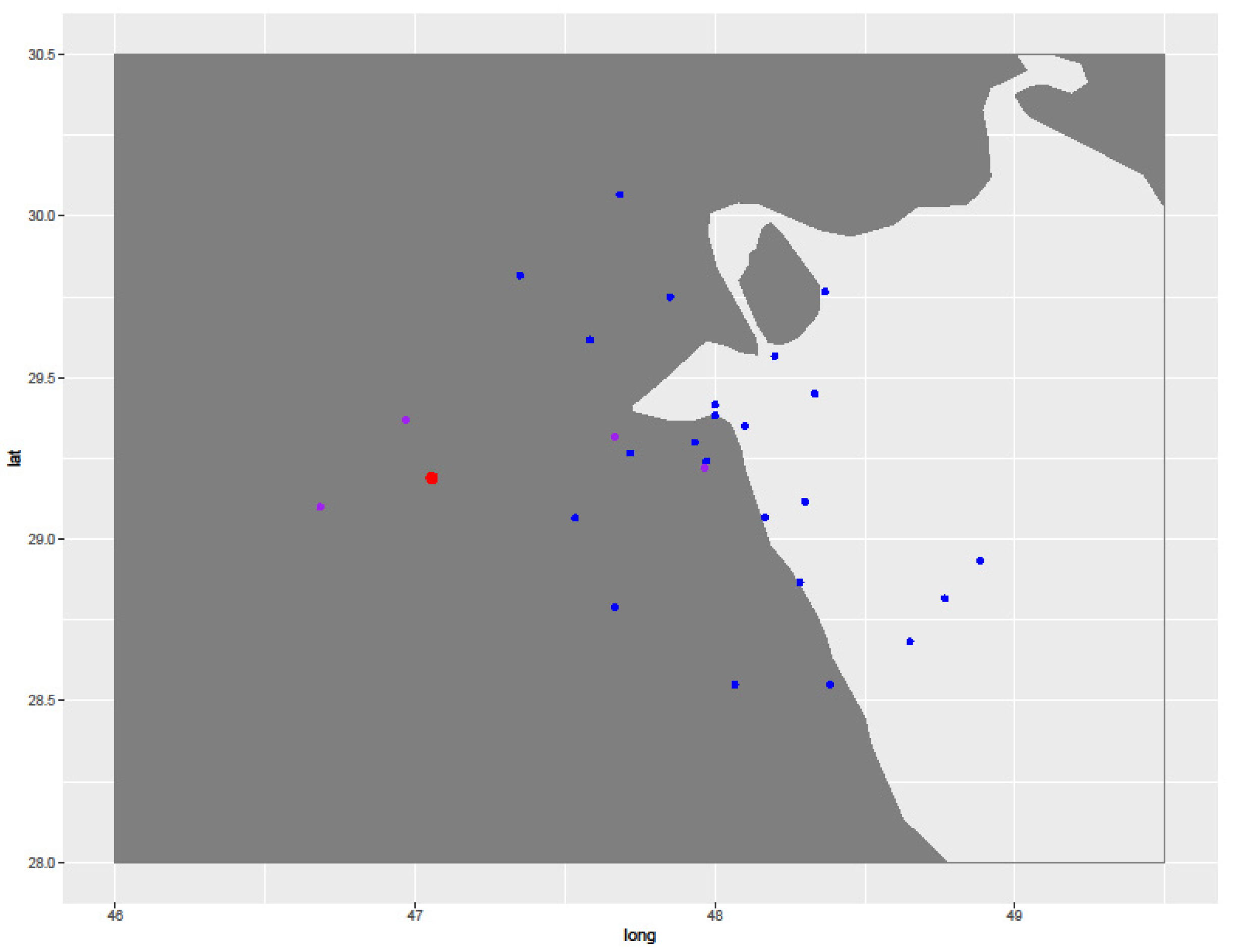
Figure 1. Location of ground-based observation stations in Kuwait: WMO Daily stations (blue); Integrated Surface Data stations (purple), Shagaya Renewable Energy Plant (red).
Energies 12 04409 g001
Figure 2. Annual distributions of (a) Subdaily and (b) daily clearness indices ( K t ) from CAMS.
Energies 12 04409 g002
Figure 3. Daily values of clearness index by month.
Energies 12 04409 g003
Figure 4. Mean Daily Clearness Indices ( K t ) by day and month for the period 2005–2017.
Energies 12 04409 g004
Figure 5. Scatter plot illustrating correlation between Daily Clearness Index ( K t ) and Daily Maximum Temperature at Abraq Mazraa (°C) for 2007–2017.
Energies 12 04409 g005
Figure 6. Mean annual daily wind observations from Shagaya Renewable Energy Park as: (a) wind roses of speed and direction by month; and frequency distributions of (b) wind direction and (c) wind speed.
Energies 12 04409 g006
Figure 7. Log likelihood values for Gaussian mixture models with 1 to 5 components.
Energies 12 04409 g007
Figure 8. Daily Clearness indices ( K t ) with three-component Gaussian mixture in red, 95% confidence intervals in dark red, and single Gaussian in grey, represented as (a) distribution densities; and (b) quantile-quantile plots.
Energies 12 04409 g008
Figure 9. Posterior probability of distribution components (dark grey) with respect to calendar day and observations (purple).
Energies 12 04409 g009
Figure 10. Mean relative humidity at 850 hPa and wind vectors (m/s) at 850 hPa associated with each distribution component, derived from ERA-Interim (2005–2017). Arrows indicate direction and magnitude of winds. Kuwait is shown with a white star.
Energies 12 04409 g010