A Two-Dimensional Study on the Effect of Anisotropy on the Devolatilization of a Large Wood Log

Abstract

In this work, a two-dimensional (2D) model for wood particle drying, devolatilization, and char conversion is presented and validated against experimental studies of devolatilization of a large, dry, cylindrical birch wood log. The wood log’s internal distributions of temperature, solid species densities, gas density, and gas species mass fractions, together with the internal pressure and the gas flow velocities in radial and longitudinal directions, were studied. It was found that the internal pressure peak significantly depended on the permeability of char. The velocity profiles changed as the pressure wave traveled radially inward in the same manner as the devolatilization zone. The wood log internal pressure was not only dependent on wood and char permeabilities but also depended on the devolatilization rate, which itself is a heat-controlled conversion stage. In addition to the study on wood anisotropy, which can be accounted for in detail by the presented 2D model, the authors compared the 2D results to results obtained from a corresponding 1D version of the model, where only radial heat and mass transfer properties were used. It was found that even though the predictions of the 2D model were in better agreement with experimental observations than the 1D modeling results, for these parameters, 1D models can still be used without too much loss in accuracy. Finally, the paper concludes with a clear recommendation of when higher dimensional models should be used and when they should not.

1. Introduction

Since 1980, the world’s primary energy consumption has dramatically increased. This increase is mainly due to an intense rise in the use of oil, coal, and natural gas [1]. Biomass can be used to generate heat via combustion, while at the same time being accompanied by limited greenhouse effects [2]. In order to confront the problems induced by greenhouse gases, i.e., global warming and climate change, research is focusing on the potential role of biomass in the future energy mix. Thermochemical degradation of biomass, from which energy carriers can be generated, and combustion, used for heat generation, are currently both intensively studied [3].

During the last years, there has been an increased focus on modeling of thermochemical wood degradation as well as on conversion of the resulting char. One-dimensional (1D) models were, and still are, one of the main tools [4]. This is because they allow for fundamental studies on conversion-related physical processes, while at the same time remaining computationally efficient. However, significant simplifications of the chemical and physical processes are required with respect to 1D model development. Multidimensional models have, on the other hand, been developed only to a very limited extent [2,5,6,7].

For both wood logs and wood chips, the original wood structure is maintained during processing. This means that both of these fuel types have a highly anisotropic structure. In 1D models, fuel properties are simplified by using radial or averaged values, i.e., by neglecting or significantly simplifying the anisotropic structure. This simplification implies, for example, that effective thermal conductivity is calculated by weighing the influence of heat transfer parallel and perpendicular to the grain direction by a bridge factor [8] and thereby significantly simplifying the anisotropic nature of wood.

Furthermore, even though research is focusing on the modeling of thermochemical wood conversion and char consumption, the developed models rarely focus on large wood logs that are comparable in size to wood logs used in wood log heating appliances (e.g., stoves and boilers [4]). There are, however, some exceptions [9,10].

A one-dimensional pyrolysis model for large wood logs (with a radius of 25 mm and a length of 300 mm) was developed by Larfeldt et al. [9]. They presented experimental data for the devolatilization of a large and dry birch wood cylinder and found a discrepancy between the modeling and experimental results. They concluded that this difference was partly due to the anisotropy of the wood, which could not be properly represented by their 1D model. A detailed description of these experiments is available in earlier work by Larfeldt [10], where wet wood logs were also tested. Furthermore, they also mention that differences in results might arise from the lack of empirical data with respect to heat transfer properties, the heat of reactions for devolatilization reactions, as well as shrinkage parameters.

Even though most models are one-dimensional, there are still a few two-dimensional studies found in the literature [2,5,6,7]. A two-dimensional (2D) drying and pyrolysis model was developed by Sand et al. [6]. They solved the momentum equations and studied a leaving gas plume that was observed during thermochemical wood log conversion. Yang et al. [5] developed a 2D combustion model. However, they only studied wood particles within a size range of 10 $\mathsf{\mu }$m to 20 mm. This size range still differs significantly from the wood logs used in domestic wood log heating appliances. Di Blasi [7] studied the anisotropy of wood by a 2D model applied to a wood slab. They found that the dynamics of particle degradation depended on the grain structure of the solid. According to their findings, an accurate prediction of the influence of anisotropy is required in order to obtain correct results for conversion time and product yields. Although it is a very nice paper, it focuses on essentially quadratic particles, which are quite different from the more rectangular shape of wood logs, and as such, this paper cannot really be used to assess the effect of anisotropy in wood logs. Pozzobon et al. [2] experimentally studied the drying and thermochemical degradation of a thermally thick wood particle exposed to a high radiative heat flux. In addition to their experiments, they developed a 2D unsteady numerical code that described drying and devolatilization in order to understand the observed phenomena. The wood samples studied in this work were small spheres with diameters in the range of 5–20 mm, which are not relevant for wood log combustion.

Even though some research has been conducted within the field of 2D modeling, 3D model development is even more limited. This is primarily due to the fact that fundamental studies of wood degradation and combustion can often be studied through lower dimensional models, which, for a given computer, are computationally faster. However, under specific conditions 3D models are necessary; e.g., when aiming for a model that describes thermochemical degradation and combustion of a wood log in a wood stack in a stove, 3D models are needed.

In general, multidimensional models are needed if:

• The wood log is subject to inhomogeneous boundary conditions. This is the case when the boundaries of the wood log are affected very differently, e.g., due to different exposure to the flame, the furnace wall, blocking by other wood logs in a stack, etc.
• The wood logs have an irregular shape, i.e., they are not cylindrical or spherical. This is typically the case for realistic wood logs as used in wood stoves.
• Wood log shrinkage is considered.
• The focus of the model is to study wood logs’ internal distributions of variables.

Even though 3D models are therefore overall recommended if they are intended to be used for describing the conversion of wood logs in wood stacks, 2D models of large wood log conversion can still serve as an intermediate development stage towards 3D models, operating faster than 3D models and capturing the anisotropy of wood more accurately than 1D models. This is why the focus of this work is on the development of 2D models. In addition to the detailed description of the extension of the earlier 1D model developed by Haberle et al. [11] to a 2D model, this work also highlights how 2D models compare against common 1D models and outperform them under specific conditions. The development of this 2D standalone code is the first step in developing a wood stove design and optimization tool. Such a detailed comparison of 1D and 2D models is not commonly presented in current literature.

In this paper, we make the same typical simplifications as made by most other groups focusing on wood log pyrolysis in order to be able to simulate such a complicated phenomenon. One could, of course, make use of, e.g., more sophisticated devolatilization models or including the surrounding fluid in the numerical meshing, but this would not result in any significant improvement in our results. The reason for this is that the main aim of our paper is to investigate the effect of wood anisotropy, and even more importantly, to study when it is relevant to use higher-dimensional models and when the much faster one-dimensional models can be used.

2. Wood Log Model

In this section, how the existing 1D model is extended to 2D is explained. First, the relevant governing equations are listed in

Table 1. List of evolution equations required for the devolatilization model. The last column gives the references the equations have been taken from.

Equation		Equation	Ref.
		Number
Wood density (1)	$\frac{\partial {\rho }_{\mathrm{w}}}{\partial t}=-(k_1+k_2+k_3){\rho }_{\mathrm{w}}-\frac{{\rho }_{\mathrm{w}}}{V_j}\frac{\partial V_j}{\partial t}$	$\left(1\right)$	[13]
Ash density	$\frac{\partial {\rho }_{\mathrm{a}}}{\partial t}=-\frac{{\rho }_{\mathrm{a}}}{V_j}\frac{\partial V_j}{\partial t}$	$\left(2\right)$	[13]
Continuity equation (3)	$\frac{\partial ϵ{\rho }_{\mathrm{g}}^{\mathrm{g}}}{\partial t}+\frac{1}{r}\frac{\partial }{\partial r}\left(r{\rho }_{\mathrm{g}}^{\mathrm{g}}{u}_{\mathrm{r}}\right)+\frac{\partial }{\partial z}\left({\rho }_{\mathrm{g}}^{\mathrm{g}}{u}_{\mathrm{z}}\right)={\dot{\omega }}_{\mathrm{g}}$	$\left(3\right)$	[7]
Species mass fraction (4)	$\frac{\partial \left(ϵ{\rho }_{\mathrm{g}}^{\mathrm{g}}{Y}_k\right)}{\partial t}+\frac{1}{r}\frac{\partial \left(r{\rho }_{\mathrm{g}}^{\mathrm{g}}{Y}_{\mathrm{k}}{u}_{\mathrm{r}}\right)}{\partial r}+\frac{\partial \left({\rho }_{\mathrm{g}}^{\mathrm{g}}{Y}_{\mathrm{k}}{u}_{\mathrm{z}}\right)}{\partial z}=\frac{1}{r}\frac{\partial }{\partial r}\left(r{\rho }_{\mathrm{g}}^{\mathrm{g}}{D}_{\mathrm{eff}}\frac{\partial Y_{\mathrm{k}}}{\partial r}\right)+$
	$\frac{\partial }{\partial z}\left({\rho }_{\mathrm{g}}^{\mathrm{g}}{D}_{\mathrm{eff}}\frac{\partial Y_{\mathrm{k}}}{\partial z}\right)+{\dot{\omega }}_k$	$\left(4\right)$	[3]
Char density (2)	$\frac{\partial {\rho }_{\mathrm{c}}}{\partial t}=k_3{\rho }_{\mathrm{w}}+ϵk_5{\rho }_{\mathrm{tar}}^{\mathrm{g}}-\frac{{\rho }_{\mathrm{c}}}{V_j}\frac{\partial V_j}{\partial t}$	$\left(5\right)$	[13]
Temperature (4)	$\left({\rho }_{\mathrm{w}}{c}_{P,\mathrm{w}}+{\rho }_{\mathrm{a}}{c}_{P,\mathrm{a}}+{\rho }_{\mathrm{c}}{c}_{P,\mathrm{c}}+ϵ{\rho }_{\mathrm{g}}^{\mathrm{g}}{c}_{P,\mathrm{g}}\right)\frac{\partial T}{\partial t}$
	$+{\rho }_{\mathrm{g}}^{\mathrm{g}}{c}_{\mathrm{P},\mathrm{g}}{u}_{\mathrm{r}}\frac{\partial T}{\partial r}+{\rho }_{\mathrm{g}}^{\mathrm{g}}{c}_{\mathrm{P},\mathrm{g}}{u}_{\mathrm{z}}\frac{\partial T}{\partial z}=$
	$\frac{1}{r}\frac{\partial }{\partial r}\left(r{\lambda }_{\mathrm{eff},\perp }\frac{\partial T}{\partial r}\right)+\frac{\partial }{\partial z}\left({\lambda }_{\mathrm{eff},\Vert }\frac{\partial T}{\partial z}\right)+{\Phi }_{\mathrm{Heat}}$	$\left(6\right)$	[14]
Radial gas velocity, $u_{\mathrm{r}}$	$u_{\mathrm{r}}=-\frac{{\kappa }_{\mathrm{radial}}}{\mu }\frac{\partial P}{\partial r}$	$\left(7\right)$	[13]
Longitudinal gas velocity, $u_{\mathrm{z}}$	$u_{\mathrm{z}}=-\frac{{\kappa }_{\mathrm{long}}}{\mu }\left(\frac{\partial P}{\partial z}+g{\rho }_{\mathrm{g}}^{\mathrm{g}}\right)$	$\left(8\right)$	[7]
Equation of state	pV = nRT	$\left(9\right)$	[7]
Effective diffusivity	$D_{\mathrm{eff}}=\frac{ϵ}{\tau }\frac{1}{\frac{1}{D_{\mathrm{AB}}}+\frac{1}{D_{\mathrm{Knudsen}}}}$	$\left(10\right)$	[11]

⁽¹⁾ The reaction rates of wood to non-condensable gases, tar, and char are given by $k_1$, $k_2$, and $k_3$, respectively. ⁽²⁾$k_5$ marks the reactions of tar to char. ⁽³⁾ Indicates that the continuity equation has been transferred to cylindrical coordinates from Cartesian coordinates. ⁽⁴⁾ Indicates that the original equation given in the reference has been extended to 2D by the authors and a correction regarding the porosity was included in the convective term.

. The presented equations only consider the devolatilization stage, since in the current test run, drying and char conversion are not modeled. Further details on the model development can be found in earlier works by Haberle et al. [11,12].

In Equation (10), one can identify that the effective diffusivity is dependent on tortuosity, which is direction-dependent. In this model, however, a simplification is made by assuming that pores are homogeneously distributed within the wood and that tortuosity can be expressed as [15]

$$\tau =\frac{1}{ϵ}.$$

(11)

Based on this simplification, the effective diffusivity is not assumed to be different in radial and longitudinal directions.

The heat-source term, ${\Phi }_{\mathrm{heat}}$, in Table 1 is defined as

$$\begin{array}{c}\hfill {\Phi }_{\mathrm{heat}}={\dot{\omega }}_{k1,k2,k3}▵h_{\mathrm{devol},1}+{\dot{\omega }}_{k4,k5}▵h_{\mathrm{devol},2}\\ \hfill +{\dot{\omega }}_{k1}\left({\int }_{T_0}^T(c_{\mathrm{P},\mathrm{wood}}-c_{\mathrm{P},\mathrm{non}-\mathrm{cond}.\mathrm{gases}})dT\right)+{\dot{\omega }}_{k2}\left({\int }_{T_0}^T(c_{\mathrm{P},\mathrm{wood}}-c_{\mathrm{P},\mathrm{tar}})dT\right)\\ \hfill +{\dot{\omega }}_{k3}\left({\int }_{T_0}^T(c_{\mathrm{P},\mathrm{wood}}-c_{\mathrm{P},\mathrm{char}})dT\right)\\ \hfill +{\dot{\omega }}_{k4}\left({\int }_{T_0}^T(c_{\mathrm{P},\mathrm{tar}}-c_{\mathrm{P},\mathrm{non}-\mathrm{cond}.\mathrm{gases}})dT\right)+{\dot{\omega }}_{k5}\left({\int }_{T_0}^T(c_{\mathrm{P},\mathrm{tar}}-c_{\mathrm{P},\mathrm{char}})dT\right)\end{array}$$

(12)

since it includes the influence of the heat of reaction of different chemical reactions as well as the changes in sensible enthalpy.

For reactions 1, 2, and 3, which describe the primary devolatilization of wood to non-condensable gases, tar, and char, respectively, the reaction rate is calculated as

$${\dot{\omega }}_{ki}=k_i{\rho }_{\mathrm{w}},$$

(13)

where ${\rho }_{\mathrm{w}}$ is the apparent wood density. The devolatilization reaction rate constants, $k_i$, are calculated from [13]

$$k_i=A_{i}exp\left(\frac{-E_{\mathrm{a},\mathrm{i}}}{RT}\right)\mathrm{for}\mathrm{i}=1,2,3,4,5,$$

(14)

with $A_i$ being the pre-exponential factor, R the ideal gas constant, T the temperature, and $E_{\mathrm{a},\mathrm{i}}$ the activation energy.

The secondary devolatilization ($i=$ 4 and 5) reaction rates are calculated as

$${\dot{\omega }}_{ki}=k_iϵ{\rho }_{\mathrm{tar}}^{\mathrm{g}},$$

(15)

with ${\rho }_{\mathrm{tar}}^{\mathrm{g}}$ being the intrinsic tar density and $ϵ$ the porosity. However, it needs to be added that tar re-polymerization to secondary char is actually a heterogeneous reaction, which is simplified to a homogeneous reaction by the kinetics implemented here. Accordingly, the consideration of secondary char formation is very much simplified, which, of course, can affect modeling results, but it is a first attempt to capture a chemical phenomenon that is not yet very well understood.

The source terms of the different gas species equations are

$${\dot{\omega }}_{\mathrm{CO}}=f_{\mathrm{CO}}{\dot{\omega }}_{{\mathrm{k}}_1}+g_{\mathrm{CO}}{\dot{\omega }}_{{\mathrm{k}}_4},$$

(16)

$${\dot{\omega }}_{{\mathrm{H}}_2}=f_{{\mathrm{H}}_2}{\dot{\omega }}_{{\mathrm{k}}_1}+g_{{\mathrm{H}}_2}{\dot{\omega }}_{{\mathrm{k}}_4},$$

(17)

$${\dot{\omega }}_{{\mathrm{H}}_2\mathrm{O},\mathrm{g}}=f_{{\mathrm{H}}_2\mathrm{O}}{\dot{\omega }}_{{\mathrm{k}}_1}+g_{{\mathrm{H}}_2\mathrm{O}}{\dot{\omega }}_{{\mathrm{k}}_4},$$

(18)

$${\dot{\omega }}_{{\mathrm{CO}}_2}=f_{{\mathrm{CO}}_2}{\dot{\omega }}_{{\mathrm{k}}_1}+g_{{\mathrm{CO}}_2}{\dot{\omega }}_{{\mathrm{k}}_4},$$

(19)

$${\dot{\omega }}_{\mathrm{tar}}={\dot{\omega }}_{k_2}-{\dot{\omega }}_{k_4}-{\dot{\omega }}_{k_5},$$

(20)

where ${\dot{\omega }}_{k_4}$ represents the reaction rate due to the tar cracking to non-condensable gases and ${\dot{\omega }}_{k_5}$ represents the reaction rate due to the tar re-polymerization to char. The fractions $f_{{\mathrm{CO}}_2}$, $f_{\mathrm{CO}}$, $f_{{\mathrm{H}}_2}$, and $f_{{\mathrm{H}}_2\mathrm{O}}$ define how much carbon dioxide, carbon monoxide, hydrogen, and water vapor are produced from primary devolatilization reactions, and the fractions $g_{{\mathrm{CO}}_2}$, $g_{\mathrm{CO}}$, $g_{{\mathrm{H}}_2}$, and $g_{{\mathrm{H}}_2\mathrm{O}}$ define how much of the corresponding species are formed from tar reactions. Those fractions are user-defined model input data.

In addition to the evolution equations, auxiliary equations are needed to describe wood properties. The effective permeabilities, ${\kappa }_{\mathrm{eff},\Vert }$ and ${\kappa }_{\mathrm{eff},\perp }$, are modeled by mass weighting the influence of primarily wood and char based on the local solid composition

$${\kappa }_{\mathrm{eff},\Vert }=\frac{{\rho }_{\mathrm{w}}}{{\rho }_{\mathrm{w}}+{\rho }_{\mathrm{c}}+{\rho }_{\mathrm{a}}}{\kappa }_{w,\Vert }+\frac{{\rho }_{\mathrm{a}}+{\rho }_{\mathrm{c}}}{{\rho }_{\mathrm{w}}+{\rho }_{\mathrm{c}}+{\rho }_{\mathrm{a}}}{\kappa }_{c,\Vert }$$

(21)

and

$${\kappa }_{\mathrm{eff},\perp }=\frac{{\rho }_{\mathrm{w}}}{{\rho }_{\mathrm{w}}+{\rho }_{\mathrm{c}}+{\rho }_{\mathrm{a}}}{\kappa }_{w,\perp }+\frac{{\rho }_{\mathrm{a}}+{\rho }_{\mathrm{c}}}{{\rho }_{\mathrm{w}}+{\rho }_{\mathrm{c}}+{\rho }_{\mathrm{a}}}{\kappa }_{c,\perp }.$$

(22)

The same permeabilities are assumed for char and ash. The effective particle emissivity, ${\omega }_{\mathrm{eff}}$, is calculated by mass weighting every solid component [13],

$${\omega }_{\mathrm{eff}}=\frac{{\rho }_{\mathrm{w}}}{{\rho }_{\mathrm{w}}+{\rho }_{\mathrm{c}}+{\rho }_{\mathrm{a}}}{\omega }_{\mathrm{w}}+\frac{{\rho }_{\mathrm{c}}}{{\rho }_{\mathrm{w}}+{\rho }_{\mathrm{c}}+{\rho }_{\mathrm{a}}}{\omega }_{\mathrm{c}}+\frac{{\rho }_{\mathrm{a}}}{{\rho }_{\mathrm{w}}+{\rho }_{\mathrm{c}}+{\rho }_{\mathrm{a}}}{\omega }_{\mathrm{a}}.$$

(23)

As Lu et al. [13] already mentioned, a volume-weighted calculation of the emissivity is more appropriate. However, this is not possible in this case due to the applied governing equations, since all solid components are assumed to occupy the same total volume. Similar challenges arise for the permeability calculation, such that mass weighting was also used for the calculation of the effective local permeability.

The effective thermal conductivities in the radial (${\lambda }_{\mathrm{eff},\mathrm{radial}}$) and longitudinal (${\lambda }_{\mathrm{eff},\mathrm{long}}$) direction are calculated as

$${\lambda }_{\mathrm{eff},\mathrm{radial}}={\lambda }_{\mathrm{cond},\mathrm{radial}}+ϵ{\lambda }_{\mathrm{rad}}$$

(24)

and

$${\lambda }_{\mathrm{eff},\mathrm{long}}={\lambda }_{\mathrm{cond},\mathrm{long}}+ϵ{\lambda }_{\mathrm{rad}},$$

(25)

with the conduction part, (${\lambda }_{\mathrm{cond},\mathrm{j}}$), being

$${\lambda }_{\mathrm{cond},\mathrm{j}}=ϵ{\lambda }_{\mathrm{g}}+(1-ϵ)\left(\frac{{\rho }_{\mathrm{w}}}{{\rho }_{\mathrm{w}}+{\rho }_{\mathrm{c}}+{\rho }_{\mathrm{a}}}{\lambda }_{\mathrm{w},\mathrm{j}}+\frac{{\rho }_{\mathrm{c}}}{{\rho }_{\mathrm{w}}+{\rho }_{\mathrm{c}}+{\rho }_{\mathrm{a}}}{\lambda }_{\mathrm{c},\mathrm{j}}+\frac{{\rho }_{\mathrm{a}}}{{\rho }_{\mathrm{w}}+{\rho }_{\mathrm{c}}+{\rho }_{\mathrm{a}}}{\lambda }_{\mathrm{a},\mathrm{j}}\right),$$

(26)

where j refers to either the longitudinal ($long$) or radial ($radial$) direction within the wood log. The calculation principle of the effective thermal conductivity was taken from Fatehi and Bai [16] but was corrected to neglect the influence of water since the wood log modeled here was perfectly dry.

2.1. Boundary Conditions

The boundary conditions at the external surfaces are modeled as described in Figure 1. The external particle surfaces (in Figure 1, the right and upper boundary) are influenced by the reactor conditions.

Due to symmetry conditions, only a part of the total wood log volume is simulated. Symmetry boundary conditions are applied (left and lower boundary), as shown in Figure 1. Heat and mass transfer coefficients, defining heat and mass transfer to the particle surface, are reduced due to the Stefan flow. The Stefan flow is an outward flow of gas that results from volatile production within the wood. The reduced heat transfer coefficient is modeled as [17]

$$h_{\mathrm{c}}=\frac{{\dot{M}}_{\mathrm{total}}{\overline{c}}_{\mathrm{P},\mathrm{g}}}{\left(exp\left(\frac{{\dot{M}}_{\mathrm{total}}{\overline{c}}_{\mathrm{P},\mathrm{g}}}{h_{\mathrm{c},0}}\right)-1\right)},$$

(27)

with $h_{\mathrm{c},0}$ being the uncorrected heat transfer coefficient, ${\dot{M}}_{\mathrm{total}}$ being the total gas phase mass flux leaving the particle, and ${\overline{c}}_{\mathrm{P},\mathrm{g}}$ being the mass-averaged specific heat capacity of the gas mixture. The mass transfer coefficient is calculated similarly as

$$h_{\mathrm{m}}=\frac{\frac{{\dot{M}}_{\mathrm{total}}}{{\rho }_{\mathrm{g}}^{\mathrm{g}}}}{\left(exp\left(\frac{{\dot{M}}_{\mathrm{total}}}{{\rho }_{\mathrm{g}}^{\mathrm{g}}{h}_{\mathrm{m},0}}\right)-1\right)},$$

(28)

with $h_{\mathrm{m},0}$ being the uncorrected mass transfer coefficient. (In earlier works by Haberle et al. [11,18], typos were unfortunately present in the definition of the corrected heat and mass transfer coefficients. The correct definition of heat and mass transfer is mentioned here, and its correctness is emphasized. The correct definition of the heat and mass transfer coefficients including the blowing effect can also be found in the literature review by Haberle et al. [4].) The Nusselt and the Sherwood number are required for the calculation of the uncorrected heat and mass transfer coefficients,

$$h_{\mathrm{m},0}=\frac{Sh{D}_{\mathrm{AB}}}{l_{\mathrm{charac}}}$$

(29)

and

$$h_{\mathrm{c},0}=\frac{Nu{\lambda }_{\mathrm{gas}}}{l_{\mathrm{charac}}},$$

(30)

with $l_{\mathrm{charac}}$ being the characteristic length. The bottom and the top of the wood log are approximated by a flat plate in a perpendicular flow at laminar flow conditions such that the corresponding Nusselt and Sherwood numbers are given by [19]

$$Nu=0.664R{e}^{0.5}P{r}^{1/3}$$

(31)

and

$$Sh=0.664R{e}^{0.5}S{c}^{1/3},$$

(32)

with the characteristic length of a the body in cross flow being defined, as suggested by Marek and Nitsche [20], as $l_{\mathrm{c}}=r$, with r being the radius of the wood log.

The lateral area of the cylindrical wood log requires a correlation that allows the calculation of the Nusselt number for a cylinder in an axial flow [21],

$$Nu=0.664\frac{P{r}^{1/3}}{\sqrt{X/4}},$$

(33)

with X defined as

$$X=\frac{\nu L}{{\left(\frac{d}{2}\right)}^2{u}_{\infty }},$$

(34)

where L is the length of the cylinder, d the diameter of the cylinder, $\nu$ the kinematic viscosity, and $u_{\infty }$ is the gas flow velocity of the bulk. Due to the analogy in heat and mass transfer, the Sherwood number can be calculated using the same correlation and substituting the Prandtl number (Pr) by the Schmidt number (Sc).

The pressure at the particle surface is set to ambient pressure. The surrounding gas phase is assumed to be pure nitrogen, i.e., Y${}_{{\mathrm{N}}_2}$ = 1, all residual Y${}_k$ = 0. The surrounding gas phase temperature is set to 973 K, which is equal to the furnace wall temperature.

The applied set of differential and algebraic equations is influenced by the choice of modeling assumptions. The 2D model development in this work is based on the following assumptions:

• The gas is ideal.
• Wood and char are anisotropic homogeneous porous media.
• Darcy’s law is used to derive the gas phase velocity, which is valid due to a low pore Reynolds number.
• Primary devolatilization is described by three independent competitive reactions, and secondary tar reactions are considered.
• The following solid and gaseous species are modeled: wood, char, ash, CO${}_2$, CO, N${}_2$, tar. No liquid species is considered since the wood log is considered to be perfectly dry.
• The solid and the gas phases are in thermal equilibrium. Therefore, it is enough to solve only one temperature equation.
• The ash content is 1 wt % (db).

2.2. Numerical Solver

The set of equations listed in Table 1 is solved by the IDA solver included in the SUNDIALS [22] software package. The advection term in the transport equations is discretized by first-order up-winding, which is sufficient for the smooth flows encountered within large wood logs. The diffusive terms in the transport equations are discretized by second-order differencing. As a consequence, the overall spatial accuracy is first-order. The IDA solver implicitly solves the set of equations by a backward differentiation formula, with the order of 1 to 5. The appropriate order is found by the solver based on the local error. The IDA solver was chosen because it follows the same concept as the DASSL solver (written in Fortran), which has already been used for thermochemical degradation modeling of wood by Grønli [3]. Since Grønli did not report any problems arising from their choice of numerical solver, it was assumed that the IDA solver can equally well lead to a suitable simulation tool for the thermochemical degradation of wood and char conversion. A grid independence study for the 1D version of a similar case to that studied here was presented in detail in Haberle et al. [11]. In the current work, we performed a similar grid independence study to validate that our resolution was high enough.

2.3. Numerical Setup

In the following, we compare our numerical results with the experimental results of Larfeldt et al. [9,10], in which dry birch wood was studied. The wood properties used in the simulations are presented in

Table 2. Properties used as input values for the devolatilization model.

Property	Unit	Value	Ref.
Thermal conductivity (wood), ${\lambda }_{\mathrm{w},\mathrm{long}}$/${\lambda }_{\mathrm{w},\mathrm{radial}}$	[W/(mK)]	0.419/0.158	[3]
Thermal conductivity (ash–fiber), ${\lambda }_{\mathrm{a},\mathrm{long},\mathrm{radial}}$	[W/(mK)]	1.2	[13]
Thermal conductivity (char), ${\lambda }_{\mathrm{c},\mathrm{long}}$/${\lambda }_{\mathrm{c},\mathrm{radial}}$	[W/(mK)]	0.1046/0.071	[7]
Thermal conductivity (gases), ${\lambda }_{\mathrm{g}}$	[W/(mK)]	25.77 × 10${}^{-3}$	[23]
Specific heat capacity (wood) (298–413 K), $c_{\mathrm{P},\mathrm{wood}}$	[J/(kgK)]	−91.2 + 4.4T	[3]
Specific heat capacity (wood) (350–500 K), $c_{\mathrm{P},\mathrm{wood}}$	[J/(kgK)]	1500 + T	[3]
Specific heat capacity (ash), $c_{\mathrm{P},\mathrm{a}}$	[J/(kgK)]	754 + 0.586 (T − 273)	[24]
Specific heat capacity (gases), $c_{\mathrm{P},\mathrm{g}}$	[J/(kgK)]	770 + 0.629 T − 1.91 × 10${}^{-4}$ T${}^2$	[3]
Specific heat capacity (char), $c_{\mathrm{P},\mathrm{c}}$	[J/(kgK)]	420 + 2.09 T − 6.85 × 10${}^{-4}$ T${}^2$	[3]
Specific heat capacity (tar), $c_{\mathrm{P},\mathrm{tar}}$	[J/(kgK)]	−100 + 4.4 T − 1.57 × 10${}^{-3}$ T${}^2$	[3]
Apparent wood density, ${\rho }_{\mathrm{w}}$ (porosity, ${ϵ}_{\mathrm{pore}}$)	[kg/m${}^3$]	410 (${ϵ}_{\mathrm{pore}}=0.4$)	[9]
Radiative thermal conductivity, ${\lambda }_{\mathrm{rad}}$	[W/(mK)]	$\frac{4\omega ϵd_{\mathrm{pore}}{T}^3}{1-ϵ}$	[3]
Binary diffusivity, D${}_{\mathrm{AB}}$	[m${}^2$/s]	3 × 10${}^{-5}$ ${\left(\frac{T}{T_{\mathrm{ref}}}\right)}^{1.75}$	[13,24]
Particle diameter, d${}_{\mathrm{P}}$	[m]	50 × 10${}^{-3}$	[9]
Aspect ratio, AR ([L/D])	[-]	6	[9]
Moisture content, M${}_{\mathrm{liquid}}$	[% wet basis]	0	[9]
Permeability, ${\kappa }_{\mathrm{w},\mathrm{long}}$	m${}^2$	2.96 × 10 ${}^{-15}$	[3]
Permeability, ${\kappa }_{\mathrm{w},\mathrm{rad}}$	m${}^2$	1.29 × 10 ${}^{-18}$	[3]
Permeability, ${\kappa }_{\mathrm{c},\mathrm{long}}$	m${}^2$	10${}^{-12}$	(1)
Permeability, ${\kappa }_{\mathrm{c},\mathrm{rad}}$	m${}^2$	10${}^{-13}$	[9]
Char emissivity, ${\omega }_{\mathrm{c}}$	[-]	0.95	[13]
Wood emissivity, ${\omega }_{\mathrm{w}}$	[-]	0.85	[13]
Ash emissivity, ${\omega }_{\mathrm{a}}$	[-]	0.85	(2)
Ash porosity, ${ϵ}_{\mathrm{pore},\mathrm{a}}$	[-]	0.8	[14]
Char porosity, ${ϵ}_{\mathrm{pore},\mathrm{c}}$	[-]	0.8	[14]
Shrinkage factor (devolatilization)	[-]	0.9	[25]

⁽¹⁾ It was assumed that the radial char permeability was smaller than the longitudinal permeability by a factor of 10. ⁽²⁾ The same emissivity was assumed for wood and ash since they were present in a solid mixture before devolatilization.

.

The pore diameter, which is required for the calculation of the radiative contribution to the effective thermal conductivity, was set to 4 × 10${}^{-5}$ m for wood and 2 × 10${}^{-4}$ m for char [3]. The pore diameter changes linearly from its value in wood to its value in char depending on the local degree of conversion, which is calculated on a mass-weighted fraction of wood or char in the total available solid phase.

It should be pointed out that the difference between radial and longitudinal char permeabilities is smaller than what could theoretically be expected. This small difference arises from numerical instabilities that were observed when larger char permeabilities were applied. The authors assume that preconditioning can be implemented in the solver to confront those instabilities. However, this is the task of future research as it goes beyond the scope of this work. Solving the momentum equation instead of Darcys law may also help to mitigate instabilities associated with large permeabilities.

Since volumetric shrinkage factors are given, how the wood log shrinks along and across the wood fibers has to be defined. Since shrinkage in the longitudinal direction is typically negligible [3], the length of the wood log is considered unchanged in this work. The wood log radius, however, decreases due to shrinkage. Based on this relative contribution of longitudinal and radial shrinkage to the volumetric shrinkage, the volumetric shrinkage calculated with the given shrinkage factor could be coupled to a definition of the radial shrinkage.

The applied pre-exponential factors, activation energies, and heat of reactions used for phase change and chemical reactions included in the model are listed in

Table 3. Kinetic data used for modeling drying, devolatilization, and char gasification and oxidation. “Gases” in the following table refers to non-condensable gases.

Reaction	Reaction Rate Constant	Unit	Ref.	Heat of Reaction [kJ/kg] (2)	Ref.
Wood → Gases	$k_1=1.11\times {10}^{11}exp\left(\frac{-177000}{RT}\right)$	[1/s]	[26]	0	(1)
Wood → Tar	$k_2=9.28\times {10}^{9}exp\left(\frac{-149000}{RT}\right)$	[1/s]	[26]	0	(1)
Wood → Char	$k_3=3.05\times {10}^{7}exp\left(\frac{-125000}{RT}\right)$	[1/s]	[26]	0	(1)
Tar → Gases	$k_4=4.28\times {10}^{6}exp\left(\frac{-107500}{RT}\right)$	[1/s]	[27]	42	[28]
Tar → Char	$k_5=1\times {10}^{5}exp\left(\frac{-107500}{RT}\right)$	[1/s]	[29]	42	[28]

⁽¹⁾ The heat of reaction was obtained by fitting the modeling results to the experimental data. ⁽²⁾ The heat of reaction is given as $▵h_i=h_{\mathrm{reactants}}-h_{\mathrm{products}}$, due to the definition of ${\Phi }_{\mathrm{heat}}$.

.

In this work, the primary devolatilization reactions were initially assumed to be endothermic, as suggested by Chan et al. [30]. Experimentally, however, we could not identify a significant temperature plateau of the center temperature in the work by Larfeldt et al. [9]. Commonly, such temperature plateaus can be observed, and their extent depends on how endothermic the primary devolatilization reactions are. Using differential scanning calorimetry (DSC) analysis, as in the work of Ciuta et al. [31], for example, who carried out DSC analysis on birch wood, the heat of pyrolysis can be studied. They found a clear heat-of-reaction neutral plateau between about 200 and 300 °C, preceded by an endothermal temperature region, after which the pyrolysis became exothermic. Due to the lack of such a temperature plateau in the experiments, it was assumed that primary devolatilization reactions are only slightly endothermic and can rather be assumed to be heat neutral. Due to this, the heat of reaction of the primary devolatilization reactions was set to zero. This assumption, with respect to the heat of reaction, is acceptable since Ström and Thunman [32] already reported that the identification of the heat of pyrolysis is challenging.

3. Results and Discussion

In this work, the 2D numerical simulation tool is used to predict the devolatilization of a large hanging wood log. The experiments, used for validation of the model, were performed by Larfeldt et al. [9]. A 2D model of the same experimental setup was already modeled by Sand et al. [6] in 2008. In the experiments, which were conducted by Larfeldt [10] (also see Larfeldt et al. [9]), the thermocouples were fixed at different radial positions (via axially drilled holes) of a wood log with a radius of 25 mm and a length of 300 mm. Besides the experimental work by Larfeldt [10], experimental research has rarely been focused on thermochemical degradation and char conversion of comparably large wood logs. This limitation in available experimental data with respect to large wood log conversion is the reason why only devolatilization of a large, dry, and hanging wood log cylinder was modeled in this work. Future modeling work is consequently also recommended to focus on the validation of the entire conversion of a large wood log, including drying, devolatilization, and char conversion. Since wood logs are thermally thick objects, devolatilization will progress inside the particle at the same time as char conversion occurs further out. The volatiles flowing out from the devolatilization zone will pass through the char and enter the surrounding fluid as an outwardly moving flow that slows down the transport of oxygen to the char conversion zone. This means that it is important that the devolatilization process is correctly represented in order predict a reasonable char conversion rate. Moreover, when the volatiles enter the surroundings, they will eventually be converted to combustion products and generate heat within the flame. The heat required for the thermal conversion of the wood log comes from this flame. So once again, if the devolatilization is not correctly handled, the rest of the conversion will also be incorrectly predicted.

In wood logs, cracks will occur during thermal conversion. These cracks may act as “highways” for advection of volatile products from the devolatilization zone to the surroundings. This means that the pressure buildup within the particle is reduced, and the volatile yield to the surroundings is concentrated around the mouth of the cracks. In between the cracks, the transport of oxygen to the char surface may now flow more easily. It should be mentioned that even though such cracks may be significant for the conversion of the log, they are hard to model and are therefore typically neglected in numerical models of wood conversion.

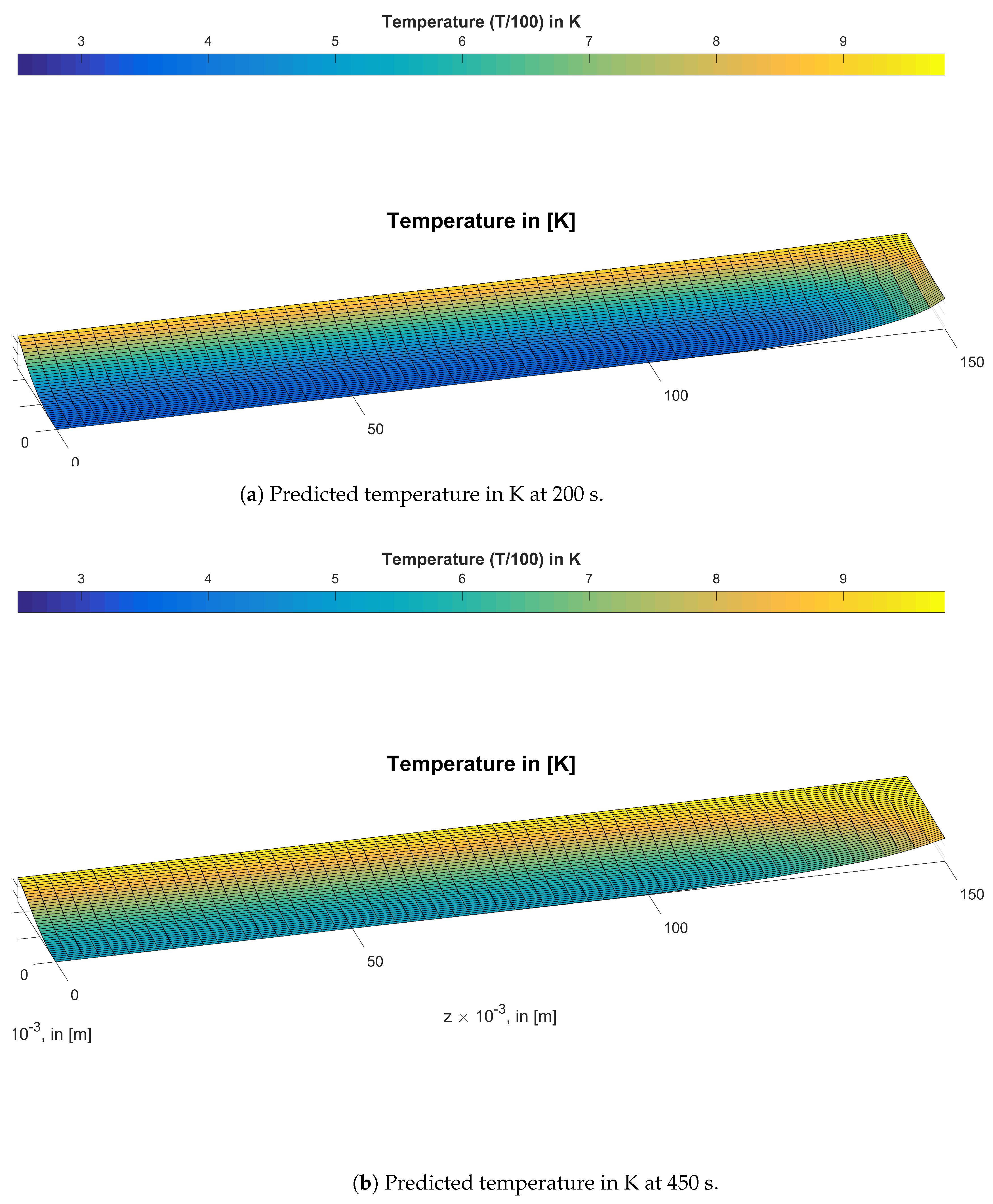
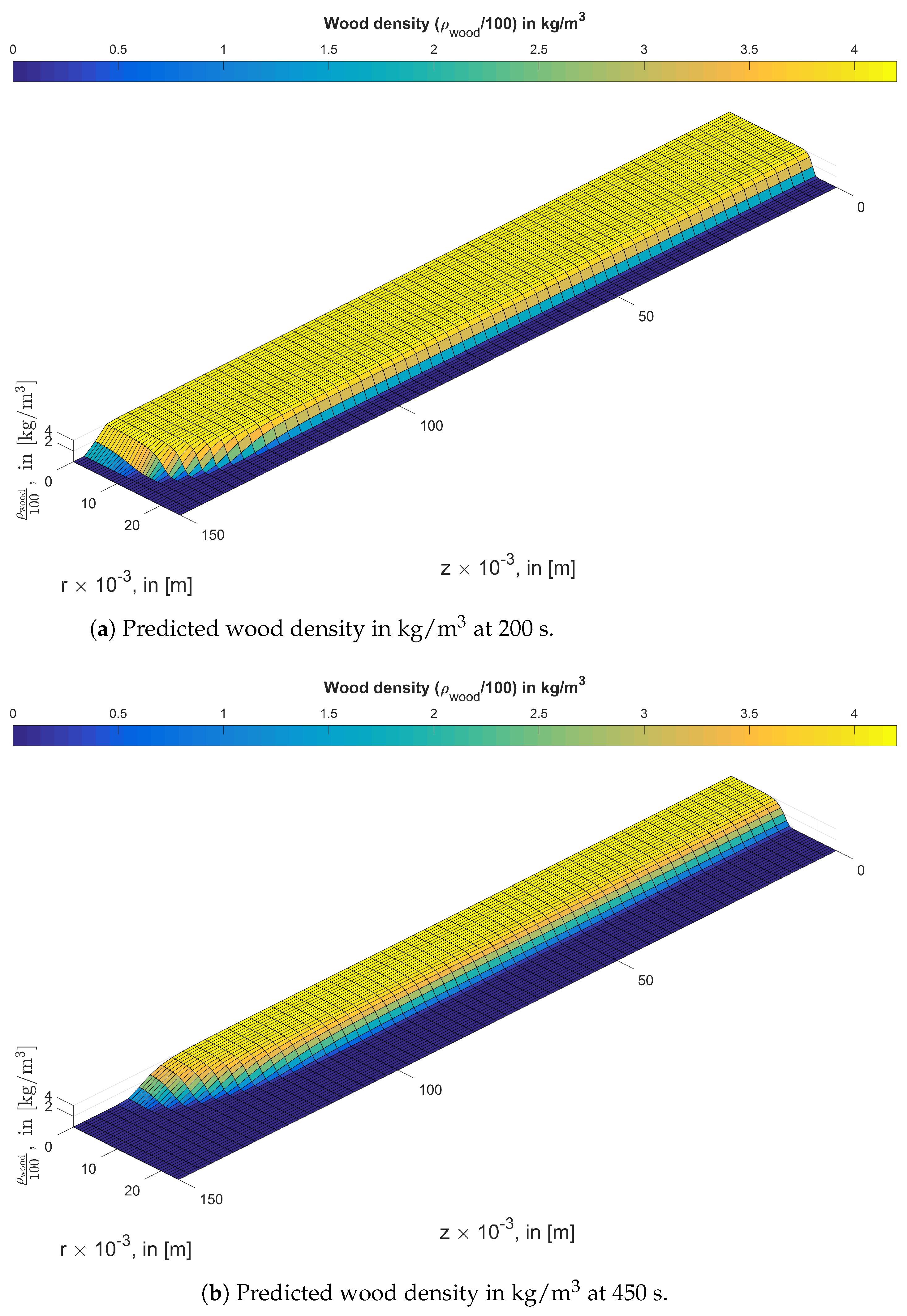
3.1. Study of the Anisotropy of Wood

In this section, the spatial distributions of temperature, densities (solid and gas), and mass fraction of tar within the modeling domain are studied, and the results at 200 s and at 450 s are shown in Figures 3–8. Due to symmetry, only a quarter of the 2D domain is considered.

The Biot number is defined as

$$\mathrm{Bi}=\frac{l_{\mathrm{charac}}{h}_c}{{\lambda }_{\mathrm{s}}},$$

(35)

where $l_{\mathrm{charac}}$, $h_c$, and ${\lambda }_{\mathrm{s}}$ are the characteristic length, the heat transfer coefficient, and the thermal conductivity of the solid, respectively. In Figure 3, it is shown that the wood log heats up from the outside, and a temperature gradient can be observed in the wood log interior. Such a temperature gradient is characteristic of thermally thick particles. This indicates that for this object, with the given heat transfer rate, the Biot number is relatively large.

In Figure 2, the different thermal conductivities of wood and char (parallel and perpendicular) used in the simulations of this paper were used for calculation of the Biot number. Different heat transfer coefficients were used for calculation. The variation in heat transfer coefficient and thermal conductivity was done to study the effect of the data on the Biot number, which by itself marks the limit between thermally thick and thermally thin wood logs. It is typically a good approximation to consider a solid object as thermally thin if the Biot number is less than 0.1. A standard value of the convective heat transfer coefficient of 20 W/(m${}^2$K) (as suggested by Fatehi [14]) was tested as a baseline case. Furthermore, a significantly smaller convective heat transfer coefficient of 2 W/m${}^2$K and the corresponding effective heat transfer coefficients of 65.43 W/m${}^2$K (with $h_{\mathrm{conv}}$ = 2 W/m${}^2$K) were compared against the baseline case. For the baseline convective heat transfer coefficient, the effective heat transfer coefficient of 83.43 W/m${}^2$K (with $h_{\mathrm{conv}}$ = 20 W/m${}^2$K) was calculated. The definition of the effective heat transfer coefficients can be found in other works [8], but it should be mentioned here that it includes both the influence of the radiative and the convective heating of the exterior of an object. Both the pure convective heat transfer coefficient and the effective heat transfer coefficient were considered in this study since they might differ significantly and therefore also significantly affect the calculated Biot number.

Except for the Biot numbers obtained for the smallest convective heat transfer coefficient and the wood thermal conductivities, all Biot numbers exceeded 0.1, which marks the critical value for thermally thick particles. Especially when considering that external heat transfer occurs via radiation and convection, as considered by the effective heat transfer coefficient, Biot numbers significantly exceed the limit of 0.1. Due to the large size of the wood log, this even applies if the diameter and length of the cylindrical wood log are divided in half. Therefore, a consequence is that if heating of the log occurs via convection and radiation, a thermally thick particle consideration is needed even for smaller log dimensions. Accordingly, one might say that due to the large log dimensions and the given simulation conditions, wood internal temperature gradients have to be well captured to accurately describe wood log conversion. Due to significant differences between perpendicular and parallel thermal conductivities, this can only be done by multi-dimensional models, which accurately represent the temperature gradients in the radial and longitudinal directions.

The temperature smoothly increases from the center to the wood log surface. Due to heat propagation from the wood log surface inward (see Figure 3), the wood starts to be consumed first at the outer areas of the wood log (see Figure 4), where the critical temperature for thermal stability of wood is reached earliest. While the wood log core still has a temperature of about 300 K at 200 s, it has already been heated up to 500 to 600 K at 450 s.

In Figure 4, the dark blue domains mark the locations in the wood log where wood has already been converted to de-polymerization products, while the wood log core (yellow domain) is still unreacted dry wood. Comparing Figure 4a and Figure 4b shows that the devolatilization front, which corresponds to the zone with a non-zero wood density gradient, propagates continuously inward. While the devolatilization zone is at about r = 20 mm (measured at centerline) at 200 s, it has proceeded to about 10–15 mm at 450 s.

Even though the thermal conductivity is higher in the longitudinal than in the radial direction, the wood is primarily converted by the devolatilization zone moving in the radial direction. This is a result of the ratio between the radial and the longitudinal dimensions of the wood log. The wood log is six times longer (L) than its diameter (D), which means that the (initial) ratio between the total surface of the devolatilization front moving in the radial ($S_R$) and longitudinal ($S_L$) directions is given by $S_R/S_L=12$. (Here, the devolatilization front is defined as the surface within the devolatilization zone with the highest primary devolatilization rate.) The result of this $S_R/S_L$ ratio is that even though the devolatilization front moves faster in the longitudinal than in the radial direction, the fact that the majority of the surface area of the combined devolatilization front is moving in the radial direction means that most of the wood devolatilization is due to the radially moving front.

In the spatial zone of low to zero wood density, one can clearly observe the notable char density increase in Figure 5.

The char density is slightly lower close to the external surface. Thermally thick particles have a faster heat transfer to the wood log surface compared to the heat transfer from the external surface to the wood log center. The outer zones of the wood log are therefore quickly heated. In those zones, more tar is formed due to competitive conversion reactions. Tar production comes at the expense of char formation. As a consequence, the char density is lower closer to the external wood log surface. As the char formation zone moves further inside, one can see that the char density forms a plateau. In the wood interior, the heat transfer further inside slows down such that the low-temperature char formation reactions dominate the devolatilization product formation. The final char yield is predicted to be about 20% of the initial dry wood log mass (see Figure 11b), which also agrees well with experimental observations.

When plotting the char densities (Figure 5), one cannot identify a char density increase towards the surface of the wood log, which would imply significant tar re-polymerization to char as tar leaves the wood log. This implies that char formation from tar in this case plays only a minor role compared to primary char formation. In fact, tar cracking to non-condensable gases is faster than secondary char formation (see Table 3). When comparing the secondary tar kinetics, one can see that even though the activation energies of the two secondary tar reaction paths are the same, the pre-exponential factor of the tar-to-char reaction is about 40 times lower than the one for tar to non-condensable gases. Therefore, the drop in tar mass fraction is primarily due to tar reacting to non-condensable gases (see Figure 8).

In Figure 6, gas densities at different spatial locations within the wood log and at different times are shown. The gas density depends on the devolatilization rate as well as wood and char permeabilities. The devolatilization rate defines the gas formation rate, while wood and char permeabilities define the mass transfer limitations and therefore the limitations of the gas flow outward. Limited outward flow at a high gas-formation rate implies accumulation of gas in the wood log structure. The combination of these two process parameters defines the peak of the gas density in the wood log interior.

In Figure 7, the wood internal pressure is shown. The pressure peak, like already discussed for the gas density peak, is the result of the gas formation rate due to primary devolatilization as well as mass transfer limitations, that is, wood and char permeabilities.

As shown in Figure 7, the pressure peak forms in the wood log center and rises from about 1.18 bar at 200 s to 1.45 bar at 450 s. When comparing the results for 200 s and 450 s, a pressure peak close to the wood log top seems to propagate inward and has reached the wood log center at 450 s. The maximum longitudinal velocities at the top of the wood log spatially occur within the area of this propagating pressure peak.

In Figure 8, the mass fraction of tar is shown at different spatial locations and at two different times (200 s and 450 s). The high tar mass fraction results from significant tar formation from primary devolatilization. The tar mass fraction drops toward the outer wood log areas. The reason for the drop in tar mass fraction is due to secondary tar cracking reactions and the dilution of tar by inward diffusion of nitrogen from the bulk flow.

In this section, it is shown that a 2D model can spatially resolve the wood’s internal distribution of different variables in sufficient detail to be able to plot internal variable fields. This spatial resolution is crucial if the location and propagation of the conversion front is to be studied in detail.

In the next section, it is shown that only a multidimensional model can accurately capture anisotropic wood properties. Furthermore, wood log dimensions affect the accuracy of modeling results and, therefore, the wood conversion prediction, making multidimensional models a prerequisite for an accurate wood log conversion simulation tool.

In order to further study the influence of anisotropy, the influence of different wood and char permeabilities on the wood internal pressure was studied. Furthermore, how the wood log dimensions affect the modeling results and whether 2D modeling becomes necessary if a certain aspect ratio is reached was studied.

3.2. Parametric Study: Wood and Char Permeability

In this section, the influence of wood and char permeability on pressure predictions is studied. The results of the parametric study are compared against the base case (see wood properties listed in Table 2), rerun with an aspect ratio of 3, as shown in Figure 9.

A second simulation was run with ten times higher char permeabilities, and the results are shown in Figure 10.

When comparing Figure 9 and Figure 10 at both times (200 s and 450 s), one can identify that the pressure peak is highly sensitive to the assigned mass transfer properties. By increasing the char permeabilities (radial and longitudinal) by a factor of 10, the pressure peak at 450 s drops significantly below the predicted pressure peak of the base case, being 1.24 bar (Figure 10) instead of 1.45 bar (Figure 9).

Furthermore, it can be observed that the propagation of the pressure peak inward is slower since the pressure peak has already reached the wood log at 450 s in Figure 9, while it is still at a position of about 8 mm in Figure 10. The different propagation of the pressure peak and its different spatial location observed from the two simulations also affects the velocity profile at the top of the wood log (compare Figure 9 and Figure 10). While the maximum longitudinal velocity at the top of the wood log has reached the wood log center (r = 0) at 450 s in Figure 9b, it is still located at about 8 mm in Figure 10b. It is also worth mentioning that a pressure peak propagating inward as shown in Figure 10b can result in radial gas transportation directed inward and outward. This is due to pressure gradients that occur on both sides of the pressure peak. As soon as the pressure peak has reached the center (as is the case in Figure 9b), the negative pressure gradient only occurs in the direction of $r_{\mathrm{inner}}\to r_{\mathrm{outer}}$, and consequently, gas transportation is only directed outward.

If the char permeability is set to higher values, implying that mass transfer is less restricted (compared to the base case), then the pressure peak propagating inward is clearly spatially differentiated (see Figure 10b). The reason is that due to the easier outflow of gases, the observed pressure peak is spatially linked to the position of the devolatilization zone since the devolatilization zone is clearly the location where significant amounts of gases are released, and the gas pressure is therefore high. Due to different time scales of chemical reactions and mass transfer, the gases are not immediately transported away after they have been formed, explaining the pressure peak at the devolatilization zone. However, convection is still high enough to avoid significant the accumulation of produced volatiles in the wood log structure, explaining why the pressure remains low at other locations further away from the immediate gas generation zone, as gases are quickly transported out of the wood log interior. Accordingly, the pressure peak as well as the wood log top velocity profile propagate inward with the devolatilization zone. For lower char permeabilities, the outward pressure gradient will be larger, which yields higher pressure peaks and hence a higher inward pressure gradient. The result is that much of the gas flows inward, creating a pressure plateau. As a result, one might conclude that if char permeabilities are set to even higher values, the pressure gradients around the inward propagating devolatilization zone will become even steeper, potentially also explaining the numerical instabilities that were encountered in this work with high permeabilities (high pressure at the grid point of gas formation, almost ambient pressure at the neighboring grid point). It is also concluded that an even larger difference between radial and longitudinal char permeabilities can significantly affect the appearance of the pressure peak and subsequently alter the velocity profiles.

Overall, the parametric study showed that the 2D model is very sensitive to the assigned permeabilities. Pressure-peak predictions as well as velocity profiles vary significantly with the choice of permeabilities. Even though the parametric study was only performed on char permeabilities, similar trends will be observed for wood permeabilities. However, they might be less visible since char permeabilities in general are significantly higher than wood permeabilities, showing a significantly higher impact on predicted mass transfer.

When comparing the results of the baseline case with a simulation case with the same permeabilities but a smaller aspect ratio (AR = 3), it can be identified that the aspect ratio also influences the wood’s internal pressure peak distribution, although not as significantly as the permeability (compare Figure 7 and Figure 9). The peak values are overall the same, being 1.18 bar at 200 s at 1.45 bar at 450 s. However, while the highest wood internal pressure can be found in the center of the wood log for a large aspect ratio, the pressure front still travels inward for the simulation case with an AR pf 3. At 450 s, the differences between the simulations with two different aspect ratios are negligible.

It is furthermore concluded that the detailed prediction of the pressure field can only be done by 2D models since the anisotropic mass transfer properties of wood and char will significantly affect the extent of the pressure peak as well as its position. Due to the strong linkage between pressure and velocity, the gas velocity profile is also highly affected by anisotropic mass transfer properties, which, as a consequence, affects the gas flow leaving the wood log. Such knowledge regarding the gas flow out of a wood log is crucial when the purpose of the simulation tool is to use it as a sub-model in a wood stove simulation tool, where not only a single wood log is to be modeled but also the interaction of a number of wood logs in a stack.

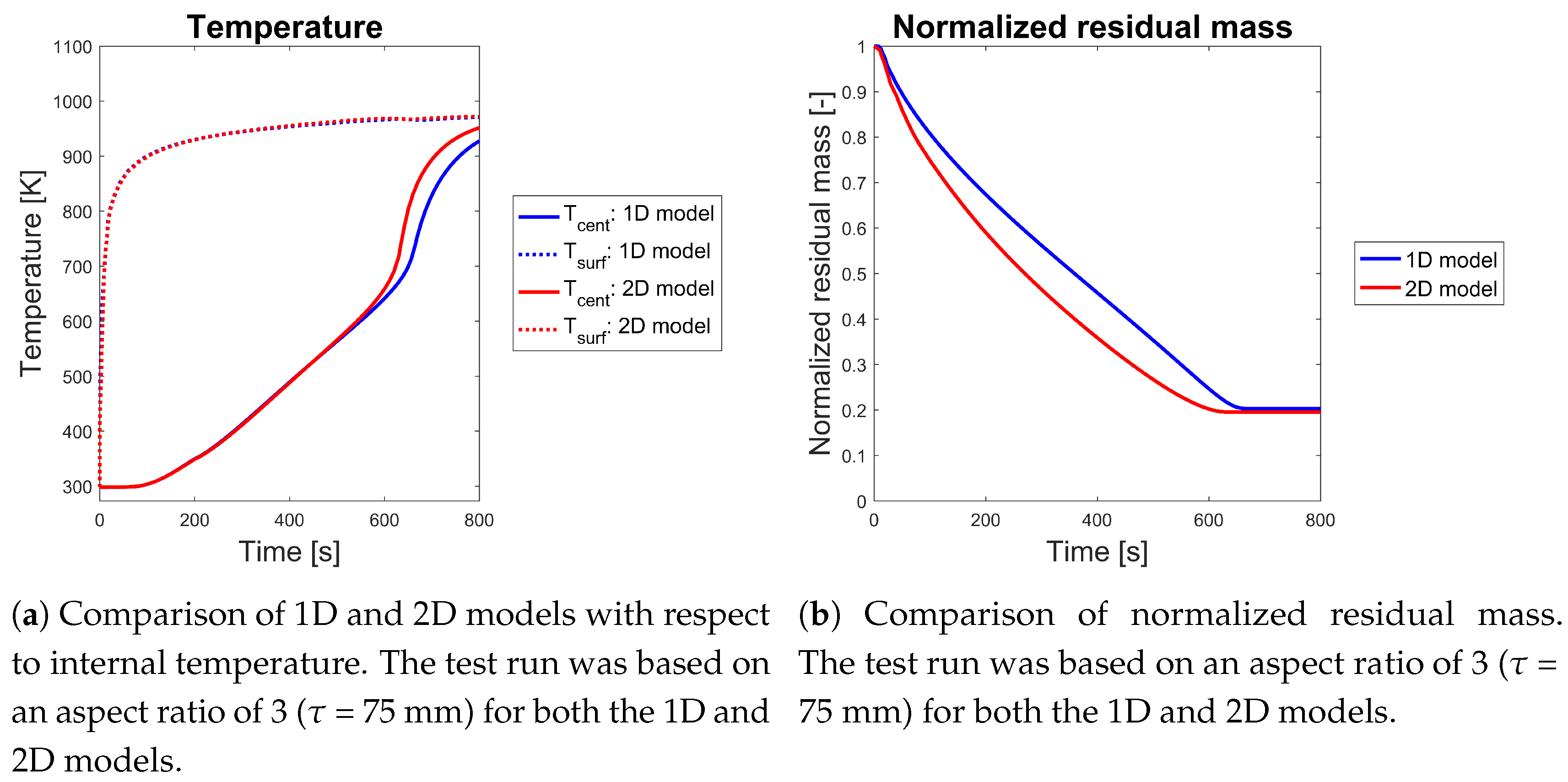
Comparison of 1D and 2D Modeling Results

The 2D model allows a detailed consideration of wood anisotropy by allowing for different heat and mass transfer properties in the radial and longitudinal directions of the wood log. However, this increase in detail comes at the cost of increased computational time. The question arises whether such a detailed model, operating at increased computational cost, is always needed to accurately predict conversion. Therefore, this section is dedicated to studying how 1D and 2D models compare in their prediction of solid degradation dynamics.

In this section, the base case presented earlier in this paper is studied. The 1D model was run purely with the radial heat and mass transfer properties of the 2D model. The results of this comparison are shown in Figure 11.

For the particular conditions that were studied in this paper, the difference in the prediction of the solid degradation dynamics between the 1D and the 2D simulations is small but notable, as shown in Figure 11. In particular, it can be seen that there is very little difference in the temperature predictions, while the difference in normalized mass is somewhat larger. The differences in normalized mass are still small compared to the overall uncertainty of the simulations, however. Therefore, it is concluded that for studying the conversion fundamentals, such as total devolatilization time as well as center and surface temperatures, a simplified 1D model is sufficient as it balances modeling accuracy and simulation time suitably well. Still, it was found that the mass loss prediction was more accurate when using a 2D model. However, this is only a valid statement for wood logs with a large aspect ratio (at least larger than 6, which was the aspect ratio of the base case). If the aspect ratio is decreased from the current value of 6, 2D models might become more relevant since the heat transfer in the longitudinal direction becomes more influential on the overall degradation dynamics. This is not necessarily the case in the base study, where the mass loss of the wood log is mostly occurring due to the inward propagation of the devolatilization zone in the radial direction.

As a consequence, how the 1D and the 2D model compare if the aspect ratio is reduced was also studied (see Figure 12).

In the following discussion, it is assumed that the 2D model is more accurate as it showed better agreement with experimental data in the base case with an aspect ratio of 6. It was found that for the modeling setup with an aspect ratio of 3, the results started to deviate significantly more. At such a low aspect ratio, not even the final conversion time can be predicted correctly with the 1D model. This highlights that multidimensional models become a necessity as the longitudinal and radial dimensions of the cylindrical wood log become more similar. Even though experimental validation cannot be done for this simulation case (AR = 3), the 1D model is obviously more wrong as it predicted the same conversion time for AR = 3 and for AR = 6. The 2D model predicted a shorter conversion time for the shorter wood log, emphasizing that it is the more accurate approach under the given conditions. The reason for this deviation in results obtained from the 1D and the 2D models is that as the influence of different dimensions on conversion is reduced, the influence of anisotropic wood properties on the overall wood conversion model predictions becomes more important.

As mentioned earlier, the 1D model still provided acceptable accuracy when applied to the numerical setup with an aspect ratio of 6 since temperature predictions did not show significant deviation, and above all, the final conversion time could still be accurately predicted, which was not the case for the test run with an aspect ratio of 3.

Independent of the aspect ratio, a 2D model will always be needed if one aims to get detailed information on wood internal distributions. Those cannot be accurately predicted by 1D models. Furthermore, inhomogeneous boundary conditions, which is what is found in wood stoves, demand multidimensional models. Moreover, if one aims to get correct volatile release rates at different positions of the wood log surface, multidimensional models are needed.

One can conclude that degradation trends obtained under simple boundary conditions, i.e., constant heat fluxes to the particle all over its surface, can be predicted well enough by 1D models, at least if the aspect ratio of the cylinder is large enough to assume an infinitely long wood log. But if one aims to couple the solid and the gas phase model to obtain an overall combustion simulation tool, multidimensional models are strictly required. This is primarily because wood logs in, e.g., wood stoves are not subject to idealized simple and homogeneous boundary conditions and also because the volatile release rate (its composition and flow rate) from the wood log is not uniform all over the wood log’s external surface. Since this volatile release enters the gas phase model, it needs to be predicted accurately in order to predict the combustion process in the wood stove correctly.

4. Conclusions and Recommendations

In this work, a 2D model for wood log devolatilization was presented. The modeling results were validated against experimental data obtained for the devolatilization of a dry, large, birch wood cylinder. Good agreement was found between modeling results and experimental data.

It was found that if wood internal variable fields are studied in detail, at least 2D modeling is needed, which can be a more computationally efficient alternative to 3D models.

How the anisotropic wood structure affects pressure magnitude and distribution, and therefore also radial and longitudinal gas velocities, was studied. It was found that the pressure peak is very sensitive to the permeabilities. The relative contribution of radial and longitudinal gas flow depends on the permeabilities in radial and longitudinal directions.

Lastly, how 1D and 2D models compare was studied. For the given case of a large wood log, solid phase degradation dynamics were acceptably well predicted by the 1D model, in particular for large aspect ratios. Nevertheless, the 2D model yielded better agreement with experiments. Since 1D models are much faster and more computationally efficient than higher dimensional models, it is important to understand how high dimensionality that is required for a given study. As a general rule, we found that higher-dimensional simulations (>1) are required when

• the wood logs have non-uniform boundary conditions (e.g., in wood stoves),
• the detailed distribution of any variable within the log is studied,
• the ratio between the longitudinal and the radial extent of the log is low,
• the log cannot be approximated as either cylindrical or spherical.

It must be highlighted that a low ratio between the longitudinal and the radial extent of the log cannot be generically quantified since the critical aspect ratio is very much case-dependent (e.g., on heating conditions). For the case modeled here, it was found that an aspect ratio of 3 already led to significant deviations between 1D and 2D modeling.

References

1. Pozzobon, V.; Salvador, S.; Bézian, J.J. Biomass gasification under high solar heat flux: Advanced modelling. Fuel 2018, 214, 300–313. [Google Scholar] [CrossRef]
2. Pozzobon, V.; Salvador, S.; Bézian, J.J.; El-Hafi, M.; Maoult, Y.L.; Flamant, G. Radiative pyrolysis of wet wood under intermediate heat flux: Experiments and modelling. Fuel Process. Technol. 2014, 128, 319–330. [Google Scholar] [CrossRef]
3. Grønli, M.G. A Theoretical and Experimental Study of the Thermal Degradation of Biomass. Ph.D. Thesis, Norwegian University of Science and Technology, Trondheim, Norway, 1996. [Google Scholar]
4. Haberle, I.; Skreiberg, Ø.; Łazar, J.; Haugen, N.E.L. Numerical models for thermochemical degradation of thermally thick woody biomass, and their application in domestic wood heating appliances and grate furnaces. Prog. Energy Combust. Sci. 2017, 63, 204–252. [Google Scholar] [CrossRef]
5. Yang, Y.B.; Sharifi, V.N.; Swithenbank, J.; Ma, L.; Darvell, L.I.; Jones, J.M.; Pourkashanian, M.; Williams, A. Combustion of a single particle of biomass. Energy Fuels 2008, 22, 306–316. [Google Scholar] [CrossRef]
6. Sand, U.; Sandberg, J.; Larfeldt, J.; Fdhila, R.B. Numerical prediction of the transport and pyrolysis in the interior and surrounding of dry and wet wood log. Appl. Energy 2008, 85, 1208–1224. [Google Scholar] [CrossRef]
7. Di Blasi, C. Physico-chemical processes occurring inside a degrading two-dimensional anisotropic porous medium. Int. J. Heat Mass Transf. 1998, 41, 4139–4150. [Google Scholar] [CrossRef]
8. Biswas, A.K.; Umeki, K. Simplification of devolatilization models for thermally-thick particles: Differences between wood logs and pellets. Chem. Eng. J. 2015, 274, 181–191. [Google Scholar] [CrossRef]
9. Larfeldt, J.; Leckner, B.; Melaaen, M. Modelling and measurements of the pyrolysis of large wood particles. Fuel 2000, 79, 1637–1643. [Google Scholar] [CrossRef]
10. Larfeldt, J. Drying and Pyrolysis of Logs of Wood. Ph.D. Thesis, Chalmers University of Technology, Göteborg, Sweden, 2000. [Google Scholar]
11. Haberle, I.; Haugen, N.E.L.; Skreiberg, Ø. Combustion of Thermally Thick Wood Particles: A Study on the Influence of Wood Particle Size on the Combustion Behavior. Energy Fuels 2018, 32, 6847–6862. [Google Scholar] [CrossRef]
12. Haberle, I.; Haugen, N.E.L.; Skreiberg, Ø. Drying of Thermally Thick Wood Particles: A Study of the Numerical Efficiency, Accuracy, and Stability of Common Drying Models. Energy Fuels 2017, 31, 13743–13760. [Google Scholar] [CrossRef]
13. Lu, H.; Robert, W.; Peirce, G.; Ripa, B.; Baxter, L.L. Comprehensive Study of Biomass Particle Combustion. Energy Fuels 2008, 22, 2826–2839. [Google Scholar] [CrossRef]
14. Fatehi, H. Numerical Simulation of Combustion and Gasification of Biomass Particles. Ph.D. Thesis, LTH (Lund University), Lund, Sweden, 2014. [Google Scholar]
15. Mehrabian, R.; Zahirovic, S.; Scharler, R.; Obernberger, I.; Kleditzsch, S.; Wirtz, S.; Scherer, V.; Lu, H.; Baxter, L.L. A CFD model for thermal conversion of thermally thick biomass particles. Fuel Process. Technol. 2012, 95, 96–108. [Google Scholar] [CrossRef]
16. Fatehi, H.; Bai, X.S. A Comprehensive Mathematical Model for Biomass Combustion. Combust. Sci. Technol. 2014, 186, 574–593. [Google Scholar] [CrossRef]
17. Bird, R.B.; Stewart, W.E.; Lightfoot, E.N. Transport Phenomena, 2nd ed.; John Wiley & Sons, Inc.: New York, NY, USA, 2002. [Google Scholar]
18. Haberle, I.; Haugen, N.E.L.; Skreiberg, Ø. Simulating Thermal Wood Particle Conversion: Ash-Layer Modeling and Parametric Studies. Energy Fuels 2018, 32, 10668–10682. [Google Scholar] [CrossRef]
19. von Böckh, P.; Wetzel, T. Erzwungene Konvektion. In Wärmeübertragung: Grundlagen und Praxis; Springer: Berlin/Heidelberg, Germangy, 2014; pp. 83–125. [Google Scholar]
20. Marek, R.; Nitsche, K. Praxis der Wärmeübertragung: Grundlagen-Anwendungen-Übungsaufgaben, 4th ed.; Carl Hanser Verlag GmbH & CO KG.: Munich, Germany, 2015. [Google Scholar]
21. Martin, H.; Gampert, B. G5-Heat Transfer to Single Cylinders, Wires, and Fibers in Longitudinal Flow. In VDI Heat Atlas; Springer: Berlin/Heidelberg, Germany, 2010; pp. 717–722. [Google Scholar]
22. National Laboratory Lawrence Livermore. SUNDIALS: SUite of Nonlinear and DIfferential/ALgebraic Equation Solvers-IDA. 2016. Available online: http://computation.llnl.gov/projects/sundials/ida (accessed on 7 April 2017).
23. Di Blasi, C. Heat, momentum and mass transport through a shrinking biomass particle exposed to thermal radiation. Chem. Eng. Sci. 1996, 51, 1121–1132. [Google Scholar] [CrossRef]
24. Hermansson, S.; Thunman, H. CFD modelling of bed shrinkage and channelling in fixed-bed combustion. Combust. Flame 2011, 158, 988–999. [Google Scholar] [CrossRef]
25. Lu, H. Experimental and Modelling Investigation of Biomass Particle Combustion. Ph.D. Thesis, Brigham Young University, Provo, UT, USA, 2006. [Google Scholar]
26. Wagenaar, B.; Prins, W.; van Swaaij, W. Flash pyrolysis kinetics of pine wood. Fuel Process. Technol. 1993, 36, 291–298. [Google Scholar] [CrossRef]
27. Liden, A.; Berruti, F.; Scott, D. A kinetic model for the production of liquids from the flash pyrolysis of biomass. Chem. Eng. Commun. 1988, 65, 207–221. [Google Scholar] [CrossRef]
28. Koufopanos, C.; Papayannakos, N.; Maschio, G.; Lucchesi, A. Modelling of the pyrolysis of biomass particles. Studies on kinetics, thermal and heat transfer effects. Can. J. Chem. Eng. 1991, 69, 907–915. [Google Scholar] [CrossRef]
29. Di Blasi, C. Analysis of Convection and Secondary Reaction Effects Within Porous Solid Fuels Undergoing Pyrolysis. Combust. Sci. Technol. 1993, 90, 315–340. [Google Scholar] [CrossRef]
30. Chan, W.C.R.; Kelbon, M.; Krieger, B.B. Modelling and experimental verification of physical and chemical processes during pyrolysis of a large biomass particle. Fuel 1985, 64, 1505–1513. [Google Scholar] [CrossRef]
31. Ciuta, S.; Patuzzi, F.; Baratieri, M.; Castaldi, M.J. Biomass energy behavior study during pyrolysis process by intraparticle gas sampling. J. Anal. Appl. Pyrolysis 2014, 108, 316–322. [Google Scholar] [CrossRef]
32. Ström, H.; Thunman, H. CFD simulations of biofuel bed conversion: A submodel for the drying and devolatilization of thermally thick wood particles. Combust. Flame 2013, 160, 417–431. [Google Scholar] [CrossRef]
Figure 1. Computational domain and applied boundary conditions. The z-axis marks the wood log length, and the r-axis marks the wood log radius. The velocity v in the figure is the same as u z in the equations, and u is the same velocity as u r in the equations.
Energies 12 04430 g001
Figure 2. Importance of accurate modeling of temperature gradients in thermally thick wood logs.
Energies 12 04430 g002
Figure 3. Wood internal temperatures in K at 200 s and 450 s during devolatilization. The top of the wood log is at z = 150 mm, and the lateral shell surface of the wood log is at r = 25 mm.
Energies 12 04430 g003
Figure 4. Wood densities in kg/m 3 at 200 s and 450 s during devolatilization. The top of the wood log is at z = 150 mm, and the lateral shell surface of the wood log is at r = 25 mm.
Energies 12 04430 g004
Figure 5. Char densities in kg/m 3 at 200 s and 450 s during devolatilization. The top of the wood log is marked at z = 150 mm, and the lateral shell surface of the wood log is at r = 25 mm.
Energies 12 04430 g005
Figure 6. Gas densities in kg/m 3 at 200 s and 450 s during devolatilization. The top of the wood log is at z = 150 mm, and the lateral shell surface of the wood log is at r = 25 mm.
Energies 12 04430 g006
Figure 7. Internal gas pressure and axial and radial gas velocities (small vectors that are most easily seen at the top of the figure). The top of the wood log is at z = 150 mm, and the initial lateral surface of the wood log is at r = 25 mm. The applied wood and char permeabilities are listed in Table 2. (Please note that the range of the color scaling is different in the two panels.)
Energies 12 04430 g007
Figure 8. Tar mass fractions [-] at different times during devolatilization. The top of the wood log is at z = 150 mm, and the lateral surface of the wood log is at r = 25 mm.
Energies 12 04430 g008
Figure 9. Internal gas pressure and axial and radial gas velocities—base case with AR = 3. The top of the wood log is at z = 75 mm (AR = 3), and the initial lateral surface of the wood log is at r = 25 mm.
Energies 12 04430 g009
Figure 10. Internal gas pressure and axial and radial gas velocities. The top of the wood log is at z = 75 mm (AR = 3), and the initial lateral surface of the wood log is at r = 25 mm.
Energies 12 04430 g010
Figure 11. Comparison of degradation dynamics predicted by the 1D model and the detailed 2D model—base case. The experimental data was read out of figures as shown in Larfeldt et al. [9]. However, to clearly distinguish between simulation results and experimental data, the experimental data are not shown as continuous lines but instead as selected values (marked by symbols).
Energies 12 04430 g011
Figure 12. Comparison of degradation dynamics predicted by the 1D model and the detailed 2D model at an aspect ratio of 3.
Energies 12 04430 g012