Optimal Operation of Battery Storage for a Subscribed Capacity-Based Power Tariff Prosumer—A Norwegian Case Study

Abstract

The cost of peak power for end-users subject to a demand charge may be substantial, expecting to increase further with the vast growth of power-demanding devices. In cases where load-shifting is not a viable option for cost reduction, battery storage systems used for peak shaving purposes are emerging as a promising solution. In this paper, the economic benefits of implementing battery storage into an existing grid-connected photovoltaic system for a medium-scale swimming facility is studied. The objective is to minimize the total cost of electricity for the facility, including the cost of energy and peak power demand, while ensuring the longevity of the battery. An optimization model based on multi-integer linear programming is built, and simulated using a one-year time horizon in GAMS and Matlab. The main results reveal that installing a battery storage system is economically attractive today, with net savings on the total system cost of 0.64% yearly. The cost of peak power is reduced by 13.9%, and the savings from peak shaving operation alone is enough to compensate for the yearly cost of the battery. Moreover, the battery ensures additional revenue by performing price arbitrage operations. When simulating the system for an assumed 2030 scenario, the battery is found to be more profitable with a yearly net savings of 4.15%.

1. Introduction

With the vast implementation of power-demanding devices, power suppliers are looking for ways to cope with supply challenges. One solution is implementing peak demand charges, encouraging end users to reduce their power demand. However, doing so in terms of shifting the load to off-peak hours is not always a viable option, especially for commercial users, as the load demand may be highly dependent on external factors. An alternative solution may be to implement battery storage for peak shaving purposes, which could reduce the cost of peak power for the end user. When subject to an hourly pricing scheme, a likely scenario in the near future due to the new smart meters, the customer could benefit further by using the battery for price arbitrage operations: the battery charges during hours of low prices and discharges when the prices are high, thus increasing its economic value.

1.1. Optimal Operation of Battery Storage

Although the costs of batteries are declining, they are still often too high for behind-the-meter applications to be economically beneficial for most customers. This, however, is often due to over-sizing the battery or its operation strategy being too simple. By optimally sizing and controlling the battery storage system to fit its application purposes, the battery can minimize its operational costs while maximizing economic benefits for the customer.

Several papers have studied the optimal operation of batteries for behind-the-meter applications, and a variety of different optimization models have been carried out. Dagdougui et al. [1] use a rule-based algorithm based on on-peak/off-peak circuits to optimize the size of a battery; however, the operational costs are excluded. Dufo-López [2] also uses a simple rule-based algorithm and real-time pricing to minimize the net present cost of the battery. Sakti et al. [3] investigate the effect of an enhanced representation of energy storage systems on the revenue from energy arbitrage over different time scales. Nottrott et al. [4] use linear programming to optimally schedule a battery while keeping the net load demand under a pre-set power limit. Although proving more beneficial than the on-peak/off-peak algorithms, the model is still too simple.

1.2. The Importance of Considering Battery Degradation

None of the papers described above consider the impact of battery degradation in their optimization models. This is true for many studies, where the lifetime of the battery is often considered to be constant regardless of how it is operated. However, the operational patterns of a battery can greatly affect its degradation process, reducing its lifetime if run too aggressively. This will in turn create a need for early reinvestments, which is largely unfavorable due to the high investment costs of battery storage.

A few papers studying the optimal operation of battery storage include degradation models in their work. Hesse et al. [5] propose a linear optimization method for cost-optimal sizing of a battery. However, the aging model is simple and the effects of power peaks are neglected. Abdulla et al. [6] propose a stochastic dynamic programming technique to optimally operate a battery, increasing the lifetime of the battery by 160% compared to non-optimal operation. However, no economics are included, and the peak demand tariffs are neglected. Ranaweera and Midtgård [7] use dynamic programming to optimize the daily operational cost, including the cost of electricity and battery degradation. However, the battery capacity is considered constant regardless of aging and the peak power tariffs are neglected. Wankmüller et al. [8] implement two different battery degradation models to investigate the impact of degradation on revenue from energy arbitrage, while neglecting both the investment cost of the battery and the peak demand tariffs.

1.3. Objective

In light of the shortcomings of the aforementioned publications, this paper aims to build a more comprehensive optimization model for end-user battery operation, considering both the degradation of the battery and the cost of peak power. With a basis in a medium-scale swimming facility, the main goal is to analyze whether implementing battery storage into an existing system can be beneficial in terms of reducing the overall system cost while ensuring the longevity of the battery. The rest of the paper is organized as follows. Section 2 presents the mathematical model of the system. Section 3 gives a brief introduction to the test case. Section 4 presents the optimization results, both at the present time and an assumed 2030 scenario, along with sensitivity analyses on important system parameters. In Section 5, the main findings from the results are discussed. Lastly, we summarize the paper with some concluding points.

2. Mathematical Model and Problem Formulations

The system can be modeled simply as a grid-connected photovoltaic (PV) + battery energy storage system (BESS) supplying a load. It should be noted that a lithium-ion battery is chosen for this study, as it is by far the most dominant technology of choice for behind-the-meter storage systems [9,10]. It is also worth mentioning that the BESS is simplified to contain only a battery bank and a bi-directional converter, and the effects of all other storage components are neglected.

A single-line diagram of the proposed system is shown in Figure 1, along with the power flows. All powers flows going into the AC bus are considered positive.

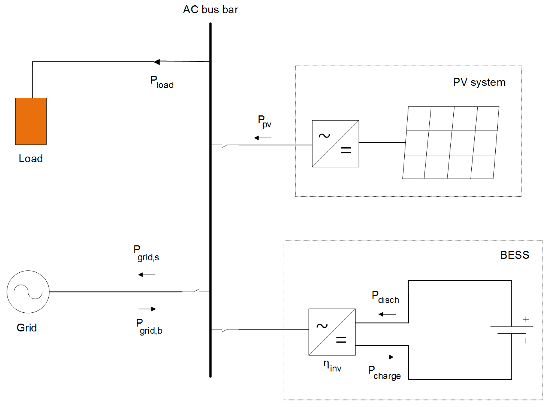
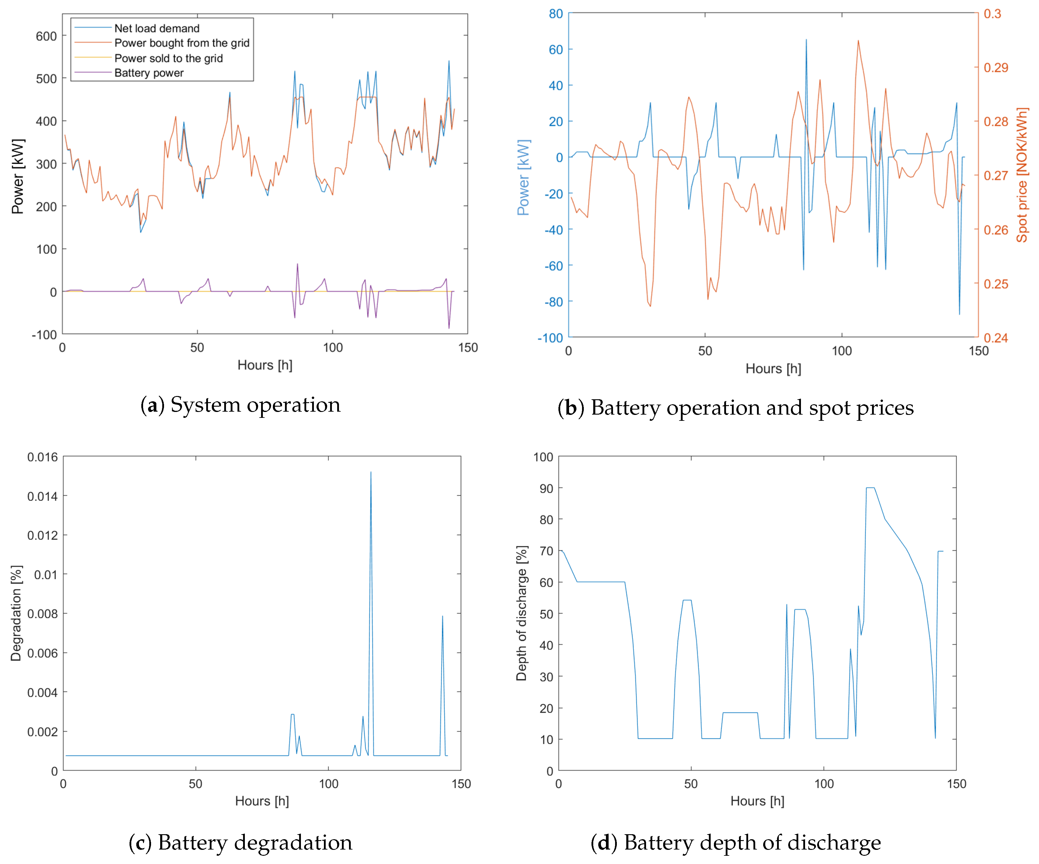
2.1. Power Balance

The most important aspect of the system is to ensure that the load demand is met at all times and that the power balance is obtained. From Figure 1, the power balance equation in time step t can be written as shown in Equation (1). $P_{pv,t}$ is the power supplied by the PV system, $P_{charge,t}$ and $P_{disch,t}$ are the powers charged and discharged from the battery, $P_{grid,b,t}$ and $P_{grid,s,t}$ are the powers bought from and sold to the grid, and ${\eta }_{inv}$ is the efficiency of the battery inverter.

$$P_{pv,t}+P_{grid,b,t}+{\eta }_{inv}{P}_{disch,t}=P_{grid,s,t}+\frac{P_{charge,t}}{{\eta }_{inv}}+P_{load,t}$$

(1)

In order to reduce the power peaks as seen from the grid, and thus enable peak shaving, a maximum limit on the power that can be drawn from the grid in any time step is applied as $P_{grid,b,t}\le P_{grid}^{max}$. Moreover, both the power bought from and sold to the grid must be of positive values, $P_{grid,b,t},P_{grid,s,t}\ge 0$.

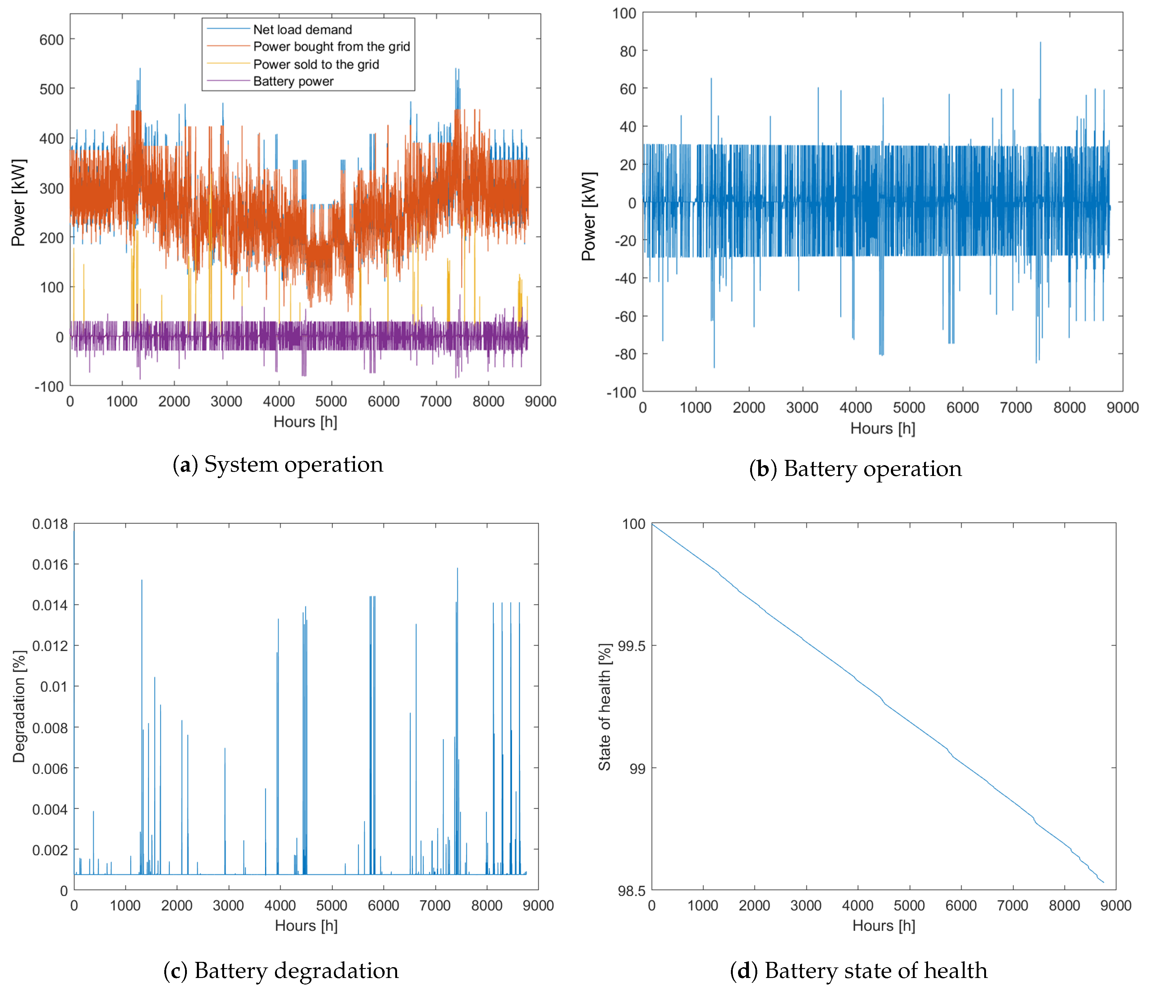
2.2. Battery Degradation

The nature of a battery is such that its usable capacity decreases as it ages. The state of health (SOH) of a battery is a measure of the current available capacity, given as a percentage of the nominal capacity. It is common to differentiate between two factors influencing the SOH; cyclic and calendric aging [11]. In addition, the aging of a battery is influenced by several operating factors, such as inefficient charging, high charging voltages and currents, deep discharging, and extreme temperatures [7].

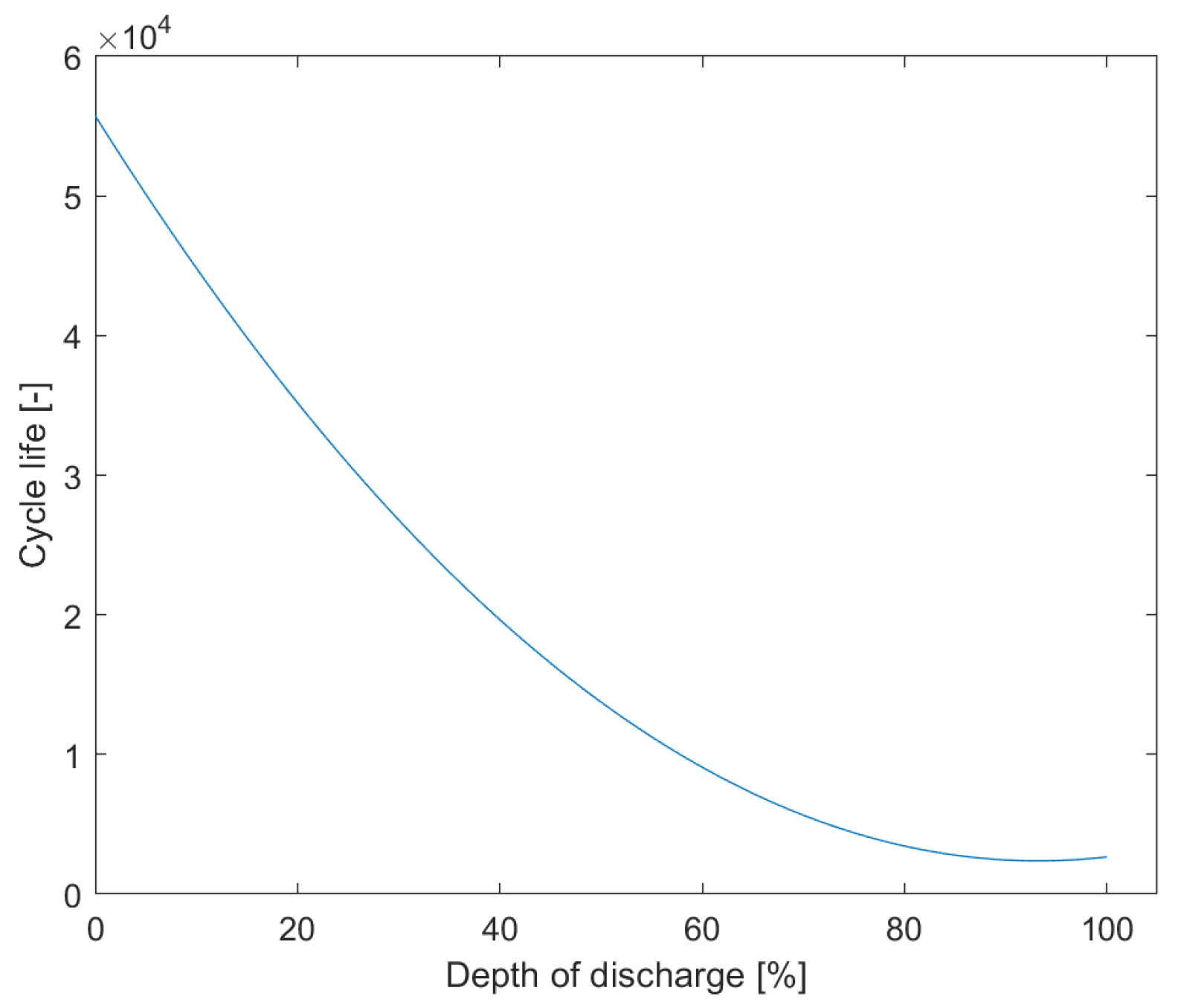
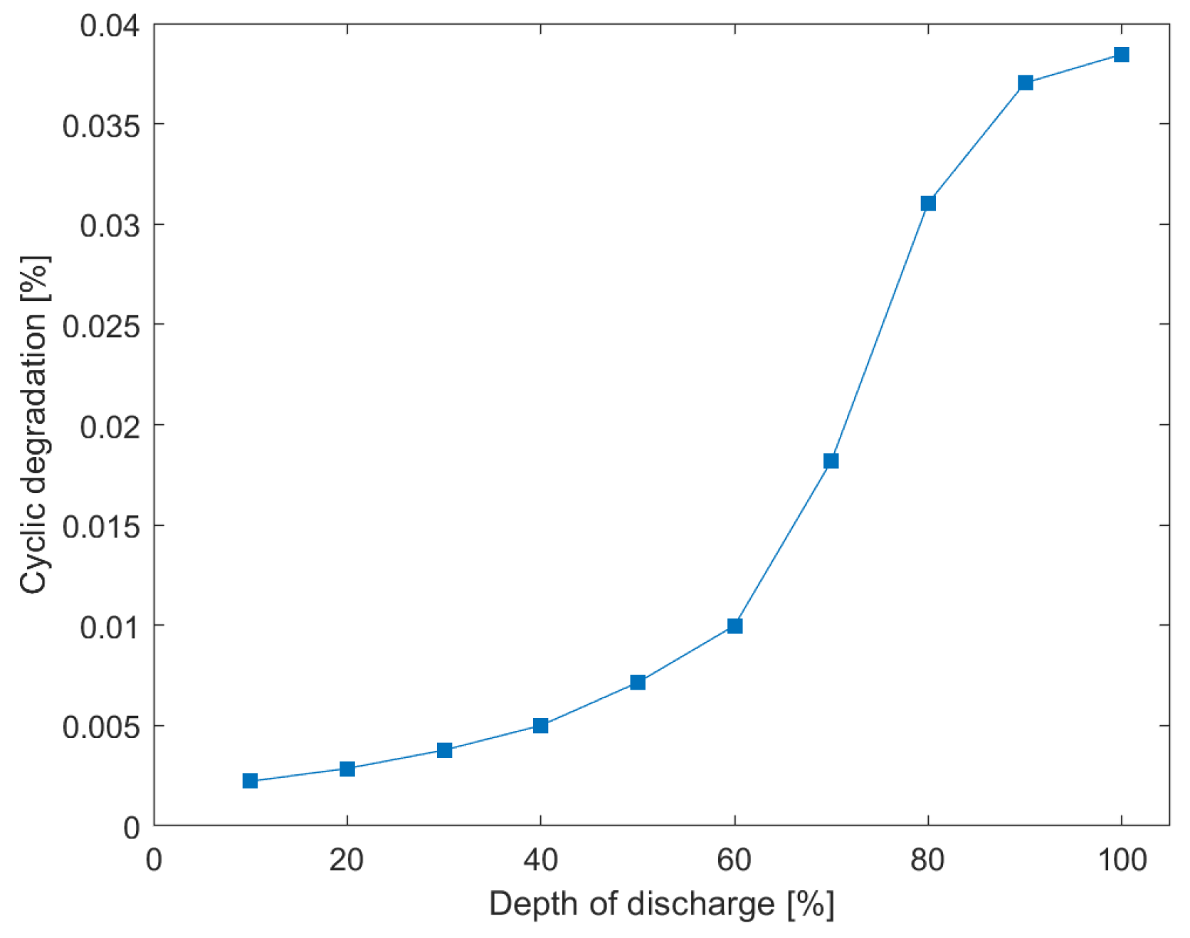
Cyclic aging is caused by energy throughput in the battery, and for each cycle the battery goes through, a certain percentage of available capacity is lost. For most lithium-ion batteries, the available capacity is sensitive to both the maximum number of full cycles and the depth of discharge (DOD) level of each cycle [12]. Figure 2 shows the number of cycles versus DOD for a nickel manganese cobalt oxide (NMC) battery, a commonly used storage chemistry for small-scale behind-the-meter applications. The figure is based on references [13,14] where a least square fitting method was applied to test data.

However, a battery is not always operated using regular cycles. This is especially true for behind-the-meter applications, where the battery operation is largely dependent on signals received from outer factors such as the energy price, power demand, and local power production [13]. It is therefore necessary to build a cyclic degradation model which reflects the irregular behavior of the battery.

Modeling the cyclic aging of a battery is difficult as it depends on both the energy throughput, cell chemistry, and operating conditions, such as temperature, cell voltage, and DOD. As such, no single model can be used for all chemistries, and a near accurate representation of the cyclic aging for each chemistry would be a highly non-linear function. Several methods have been proposed [15,16]; however, the model used in this paper is based on the curve from Figure 2: the degradation of each regular cycle, i.e., when discharging the battery from full capacity to a specified DOD level, is modeled as ${\rho }_t=\frac{100\%}{L_{cyc}}$, where L_cyc is the cycle life of the resulting DOD and ${\rho }_t$ is the percentage degradation in time t. A similar model is also used by References [13,17]. Although being cell specific, it can easily be adapted to fit all chemistries where such a curve is available and can therefore produce accurate results for the chosen battery technology.

As previously mentioned, it is desirable to build a model which accounts for irregular battery cycles. In the paper by Wang et al. [13], an irregular cycle is modeled as the difference between two regular cycles, as follows:

$$D{P}_{cyc,t}=0.5|{\rho }_t-{\rho }_{t-1}|$$

(2)

Here, DP_cyc represents the degradation in each time period. The absolute value is due to the fact that both charging and discharging contributes to a degradation of the battery, and the factor of 0.5 reflects that one charging or discharging process contributes to half of the degradation of a full cycle.

As opposed to cyclic aging, calendric aging is independent of energy throughput and comprises all internal processes leading to the degradation of a battery when idle. The capacity lost during these idle intervals is mainly dependent on the storage state of charge (SOC) and temperature. Several papers ([15,18]) have studied the change in the SOH for lithium-ion batteries when storing them at different temperatures and SOCs and found that the calendric aging did not increase linearly with the SOC, nor with temperature. By assuming a constant temperature, the model can be simplified, and several sources ([5,19]) propose a solely time-dependent model of the calendric aging. In this paper, the degradation in each time step is expressed as $D{P}_{cal,t}=\frac{100\%}{L_{cal}}$, where L_cal is the shelf time of the battery given by the manufacturer.

Both the cyclic and calendric aging affect the SOH of the battery. With the total degradation expressed as DP, the battery is at the end of its lifetime for DP = 100%. If the end-of-life criterion is set to 80% of full capacity, a typical replacement criteria for lithium-ion batteries, the SOH of the battery in each period can be modeled as $SO{H}_t=SO{H}_{t-1}-0.2D{P}_t$, where DP_t is the total degradation in per unit in time period t.

According to the state of the art, the total degradation of the battery can be modeled in several ways. Some articles ([5,20]) model the total aging as a superposition of the cyclic and calendric aging, while others ([7,15]) argue that the two processes are independent of each other: the total aging is equal to DP_cyc if the battery is operating, and DP_cal if it is idle, as seen in Equation (3):

$$DP=\left\{\begin{array}{cc}D{P}_{cal},\hfill & P_{charge}=P_{disch}=0\hfill \\ D{P}_{cyc},\hfill & \mathrm{otherwise}\hfill \end{array}\right.$$

(3)

Other articles again ([13,19]) argue that the total degradation in each period can be modeled as the larger one of the two aging processes. If DP_cyc is higher than DP_cal for all DOD levels, and noting that DP_cyc is equal to zero when the battery is idle, this approach can be seen as a simplification of Equation (3). The resulting model is:

$$D{P}_t=\max \{D{P}_{cyc,t},D{P}_{cal,t}\}$$

(4)

2.3. The Cost of Battery Storage

By assuming that the degradation cost is a percentage of the initial investment cost, such that when the battery reaches the end of its lifetime the initial investment is accounted for, the degradation cost can be expressed $\gamma =C_{bat}DP$ ([17]), where C_bat is the initial cost of the battery. The initial cost is highly dependent on the size of the battery, $C_{bat}=c_{bat}{E}_{bat}^{nom}$, where c_bat is the specific cost in NOK per capacity and $E_{bat}^{nom}$ is the nominal capacity of the battery.

As seen from these equations, the degradation cost of the battery is strongly affected by the initial investment cost, which in turn varies greatly for each cell chemistry: today’s average prices for a BESS can range from NOK 2800 to NOK 8400 per kWh (based on conversion from USD to NOK, with an exchange rate of 8.00 NOK/USD). However, with increasing deployment of li-ion batteries in various applications worldwide, costs are rapidly declining: in a study by the International Renewable Energy Agency (IRENA) from 2017, average battery system costs are expected to lie between NOK 1000 and NOK 2800 per kWh in 2030 [10]. These estimations are further backed up by Bloomberg New Energy Finance [21].

2.4. The Cost of Energy

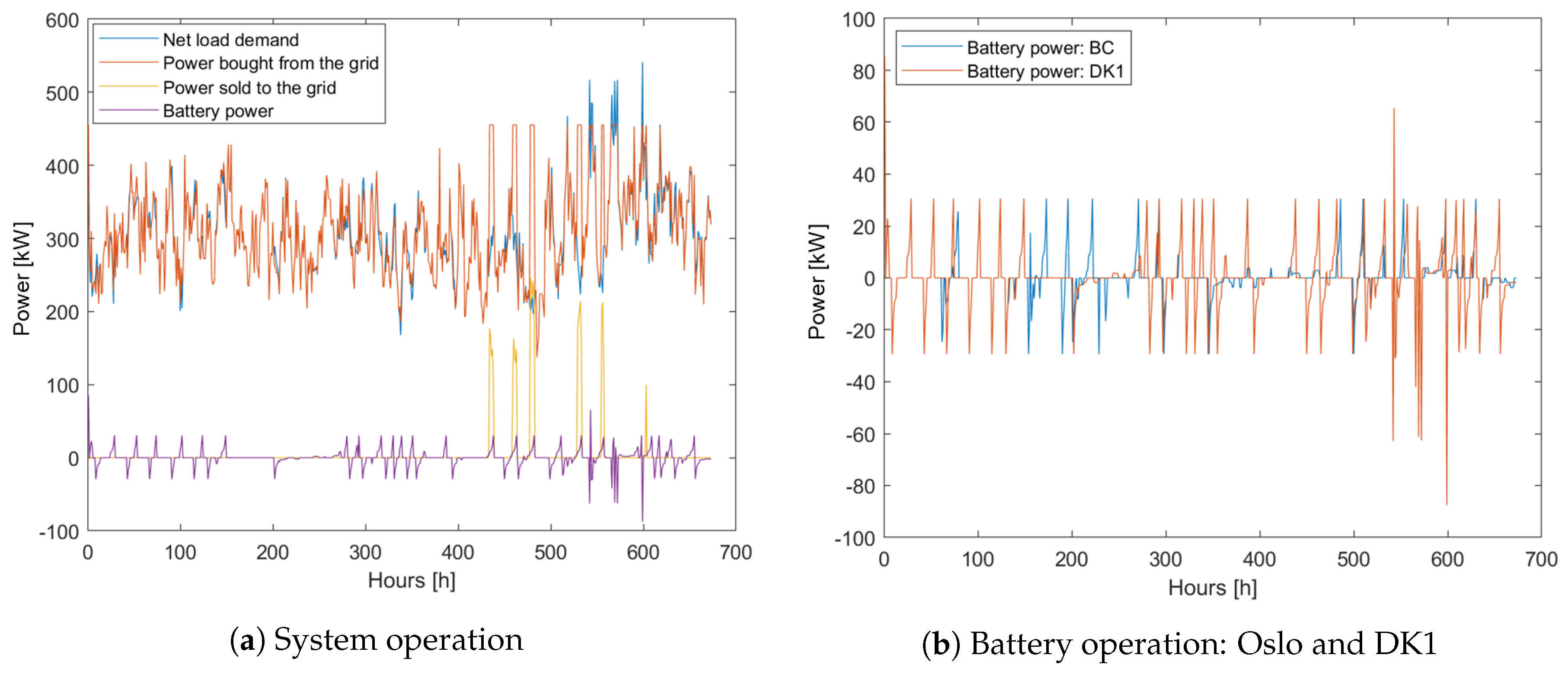
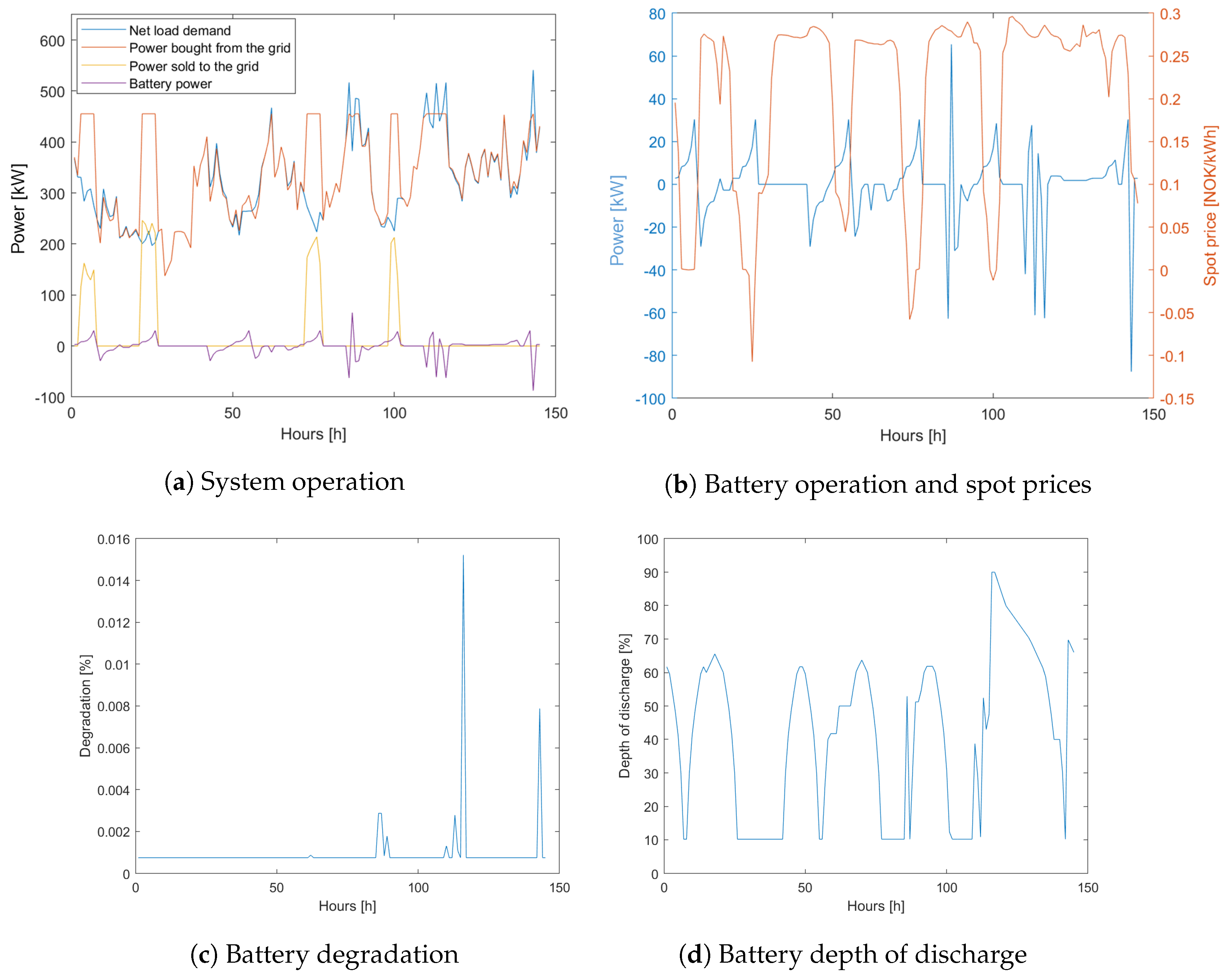
Each kWh of energy delivered through the grid is subject to an energy tariff, which can be either a flat rate or a time-dependant rate. Traditionally, the flat rate is the most widespread tariff scheme in Norway. However, with the introduction of smart meters the consumers will be more exposed to price signals in the power market, and time-based tariffs may become increasingly deployed: instead of charging a constant price, the cost per kWh is dependent on the time in which that kWh is used. One way of implementing this is to base the energy tariff on hourly rates equal to the spot prices, called “real-time pricing” (RTP). In Norway these rates are decided by Nord Pool [22]. Under an RTP tariff scheme, battery storage systems may prove economically valuable as they can be used for price arbitrage operations. This is especially beneficial for areas where the difference between on and off-peak energy tariffs are high, which may be the case for Norway in the near future. According to a study made by Statnett last year, the Norwegian spot market will see more volatile prices and higher price peaks as the implementation of fluctuating power sources like solar and wind continue to grow [23].

In addition to being charged for each kWh of energy consumed, commercial customers are subject to a peak demand charge—a fee charged for the maximum power drawn from the grid each billing period. This charge may be of a substantial amount and is set high to reflect that the consumption peaks cause a stress on the grid.

The total cost of electricity for each billing period can be modeled as shown in Equation (5), where t indicates hours and T is the last hour of the billing period. c_el,t is the energy tariff, c_feed-in,t is the feed-in tariff, and c_peak is the peak demand charge. P_grid,b,t is the power bought from the grid each hour, P_grid,s,t is the power fed back (or sold) to the grid each hour, and P_peak is the maximum amount of power drawn from the grid during the billing period.

$$C_{el}=\sum _t^T(c_{el,t}{P}_{grid,b,t}\Delta t-c_{feed-in,t}{P}_{grid,s,t}\Delta t)+c_{peak}{P}_{peak}$$

(5)

2.5. Battery Model

When the battery is operating, it can either charge or discharge—but never both at the same time. In each time step, the charging or discharging powers are limited by the nominal power of the bi-directional inverter to avoid over-voltages and high currents, $0\le P_{charge,t}\le {\eta }_{inv}{P}_{inv}^{nom}$ and $0\le P_{disch,t}\le P_{inv}^{nom}$. In each operating period, the energy in the battery is either increased or reduced according to Equation (6). Note that when the battery is idle, P_charge,t = P_disch,t = 0 and the energy content remains unchanged.

$$E_{bat,t}=E_{bat,t-1}+{\eta }_{charge}{P}_{charge,t}\Delta t-\frac{P_{disch,t}}{{\eta }_{disch}}\Delta t$$

(6)

The charging and discharging efficiencies depend on the current through the battery; however, for simplification they are assumed constant throughout the simulation. Furthermore, it is assumed that the efficiencies are equal and that they can be calculated based on the battery round-trip efficiency ($\eta rt$) [2,5,7], ${\eta }_{charge}={\eta }_{disch}=\sqrt{{\eta }_{rt}}$.

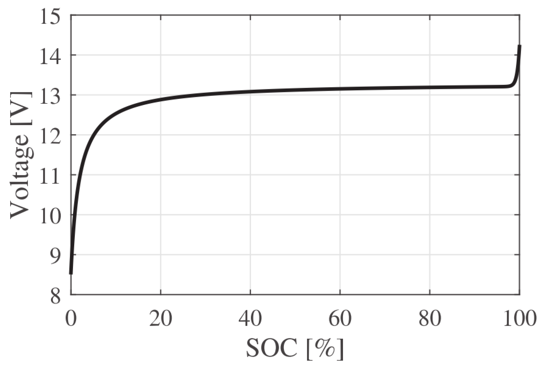
The available energy in time t is controlled by the usable capacity as well as the minimum and maximum levels of the state of charge, $E_{bat,t}^{usable}SO{C}_{min}\le E_{bat,t}\le E_{bat,t}^{usable}SO{C}_{max}$, where $SO{C}_{max}$ and $SO{C}_{max}$ are given as percentages. This is set to avoid overcharge or deep discharge. As seen in Figure 3, the open circuit voltage of a lithium-ion battery is relatively constant in the SOC range of 10%–90%, so operation in this region is preferable. For this study, the battery voltage is assumed to be constant over the whole charge and/or discharge cycle.

As discussed in Section 2.2, the battery deteriorates due to aging. As such, the usable capacity decreases with each time step according to the state of health: $E_{bat,t}^{usable}=E_{bat,t}^{nom}SO{H}_t$, where $SO{H}_t$ is given as the percentage of nominal capacity remaining in time t. The resulting limits on the energy content are shown below:

$$E_{bat}^{nom}SO{H}_{t}SO{C}_{min}\le E_{bat,t}\le E_{bat}^{nom}SO{H}_{t}SO{C}_{max}$$

(7)

The SOC and the energy of the battery are interdependent, and the SOC can be expressed as:

$$SO{C}_t=\frac{E_{bat,t}}{E_{bat,t}^{usable}}=\frac{E_{bat,t}}{E_{bat}^{nom}SO{H}_t}$$

(8)

In addition, as previously mentioned, the SOC is limited to its minimum and maximum levels: $SO{C}_{min}\le SO{C}_t\le SO{C}_{max}$. The DOD of the battery is dependent on the SOC, and vice versa, and it is defined as: $DO{D}_t=1-SO{C}_t$.

2.6. The Objective Function

The objective of the model is to minimize the total system cost while satisfying the constraints described above. The system cost consists of two parts: the total cost of electricity and the operational cost of the battery. The operational cost of the battery is assumed to only include the cost of degradation, hence maintenance costs are neglected. Based on Equation (5), the total cost of electricity can be modeled as:

$$C_{el}=\sum _{t\in T}(c_{el,t}{P}_{grid,b,t}\Delta t-c_{feed-in,t}{P}_{grid,s,t}\Delta t)+\sum _{m\in M}\left(c_{peak,m}{P}_{peak,m}\right),$$

(9)

where P_peak,m is the maximum power drawn from the grid in time t within month m, given as: $P_{peak,m}\ge P_{grid,b,t}\forall t\in M$. The total degradation cost of the battery can in turn be modeled as: $C_{deg}={\sum }_{t\in T}{\gamma }_t$, where $\gamma t$ is the degradation cost in each time step, defined in Section 2.3. Considering the equations given above, the objective function becomes:

$$\begin{array}{c}{\displaystyle \underset{\begin{array}{c}\forall t\in T\\ \forall m\in M\end{array}}{min}}{C}_{tot}(t,m)=\\ {\displaystyle \sum _{t\in T}}(c_{el,t}{P}_{grid,b,t}\Delta t-c_{feed-in,t}{P}_{grid,s,t}\Delta t+{\gamma }_t)+{\displaystyle \sum _{m\in M}}\left(c_{peak,m}{P}_{peak,m}\right)\end{array}$$

(10)

2.7. Linear Programming

The objective function and most of the equations and constraints have linear relationships, making linear programming (LP) well suited to solve the optimization problem. It should be noted that some of the equations and constraints have been simplified in order to obtain a model which can easily be solved to find the optimal solution. In reality, these models of real life scenarios may be much more complex. Nevertheless, the simplifications can be justified as linear optimization provides unambiguous, repeatable results without requiring large computational efforts as compared to other optimization methods [5].

The battery degradation model contains non-linear parts. Seeing as LP requires all equations and constraints to be linear, linearization needs to be applied. Referring to Reference [13], the non-linear Equations (2) and (4) are linearized as follows: Equation (2) is transformed into $D{P}_{cyc,t}\ge 0.5({\rho }_t-{\rho }_{t-1})$ and $D{P}_{cyc,t}\ge 0.5(-{\rho }_t+{\rho }_{t-1})$, and Equation (4) is transformed into $D{P}_t\ge D{P}_{cyc,t}$ and $D{P}_t\ge D{P}_{cal,t}$. However, there are still non-linearities in this model: when looking at Figure 2, it becomes evident that there is a non-linear relationship between the DOD and the cycle life of the NMC battery. Seeing as the cyclic degradation, $\rho t$, is defined as the inverse of the cycle life, Equation $D{P}_{cyc,t}\ge 0.5({\rho }_t-{\rho }_{t-1})$ and $D{P}_{cyc,t}\ge 0.5(-{\rho }_t+{\rho }_{t-1})$ contain non-linear parts and need to be further linearized.

In order to model the non-linear relationship between the cyclic degradation and DOD, piecewise linearization is applied to the inverse of Figure 2: the curve is divided into n linear segments, connected through n + 1 points, as seen in Figure 4. For a specific DOD value located between two points, the resulting degradation percentage is found based on the linear function of the segment connected by these two endpoints. In LP, this can be modeled by using special order sets of type 2 (SOS2). An SOS of type 2 is an ordered set of variables, where at most two variables can be non-zero for each time period. If two variables are non-zero, these must be adjacent. A linear model containing such sets becomes a discrete optimization model, even though the members of the set may be continuous. As such, a mixed integer linear optimizer is required to solve the problem [24].

The piecewise linearization using SOS2 is done through: ${\rho }_t={\sum }_{i\in I}de{g}_{t,i}{w}_{t,i}$, $DO{D}_t={\sum }_{i\in I}do{d}_{t,i}{w}_{t,i}$ and ${\sum }_{i\in I}{w}_{t,i}=1$, where index i indicates point i on the piecewise linear curve. Here, deg_t,i represents the degradation, dod_t,i the depth of discharge, and w_t,i the SOS2 variable of point i. The SOS2 property of having at most two non-zero variables which have to be adjacent, ensures that we are always on the piecewise linear function. This could also have been modeled using binary variables; however, special ordered sets are usually preferred as they may provide significant computational savings [24].

2.8. Overall Optimisation Framework

The overall optimisation framework is elaborated in Figure 5.

3. Case Study

The system under study is a Norwegian medium-scale swimming facility, more specifically Holmen swimming facility. With 45% annual energy savings (compared to swimming facilities built according to today’s regulations) and a PV system covering around 12% of the annual electricity demand, it is considered a passive house and is one of the countries most energy efficient swimming facilities [25]. However, their power peaks are high, meaning their total cost of electricity may be substantial even with the annual energy savings.

In order to capture the seasonal characteristics with regards to PV generation and load demand, a planning horizon of one year with hourly time increments is considered in the simulations. A time resolution of one hour was chosen based on the energy market operating on an hourly basis, and it is a compromise between obtaining accurate results and lowering the computational speed. The mathematical model of the system, presented in Section 2, is written in The General Algebraic Modeling System (GAMS) and solved using Gurobi. Below, important system parameters are presented.

3.1. The Cost of Electricity

The cost of electricity is based on tariffs set by the local network company, Hafslund Net. The energy tariff is assumed to be time dependent to reflect the near future trends, as presented in Section 2.4. More specifically, an RTP scheme is chosen, based on the Elspot day-ahead prices for Oslo in 2017, collected from Nord Pool [26]. A revenue from selling power to the grid may be generated if the solar production exceeds the load demand. For this study, a constant value of 0.04 NOK per kWh is chosen based on the feed-in tariff provided by Agder Energy [27]. The cost of peak demand is subject to the charges presented in

Table 1. Peak demand tariffs, based on data from Hafslund Net [28].

Demand Tariffs
Winter 1 (Jan., Feb., Dec.)	150 NOK/kWp/month
Winter 2 (Mar., Nov.)	77 NOK/kWp/month
Summer (Apr.–Oct.)	11 NOK/kWp/month

as of 2018, based on data from Hafslund Net [28].

3.2. Estimating Yearly Load and Production

For the swimming facility, no recorded data on load demand and solar production is available before January 2018. Thus, in order to be able to analyze the system behavior for one full year, estimates on future demand and production have been made. The yearly load demand was estimated using historical data from January to April 2018 and load demand trends from other swimming facilities in Norway [29], while the PV production was calculated using PVWatts^® Calculator and actual system parameters.

3.3. Estimating $E_{bat}^{nom}$ and $P_{grid}^{max}$

Both the nominal battery capacity, $E_{bat}^{nom}$, and the maximum amount of power that can be drawn from the grid, $P_{grid}^{max}$, are parameters in the optimization model, meaning they are set prior to solving. Seeing as these values may have a large effect on the resulting system costs, it is important to decide on their near-optimal values before solving. In order to find these values, simulations of the proposed system were carried out with a one month time horizon for different values of $E_{bat}^{nom}$ and $P_{grid}^{max}$. A one month time horizon was chosen as it significantly reduces the simulation time when compared to one year, while still being able to include the peak demand charge. The month with the highest peak was chosen to capture the most extreme scenario, which in this case was February.

The simulation steps are listed below. Note that the values from

Table 2. Parameter values used for the simulations. (a) System parameters; (b) Simulation parameters.

(a)
Parameter	Value
Pload,t	Input data
Ppv,t	Input data
cel,t	Day-ahead prices, Oslo (2017)
cfeed-in,t	0.04 NOK/kWh
cpeak,m	See Table 1
$P_{inv}^{nom}$	150 kW
$E_{bat}^{nom}$	150 kWh
$\eta inv$	98%
$\eta rt$	96%
SOCmin	10%
SOCmax	90%
Lcal	15 years
cbat	3600 NOK/kWh (Based on cost estimates of NMC BESS for 2016 [10])
(b)
Parameter	Value
T	8760
M	12
$\Delta t$	1 h
$P_{max}^{grid}$	455.38 kW
$E_{init}^{bat}$	0 kWh
SOHinit	100%

were used.

• The system was simulated for a given, constant value of $E_{bat}^{nom}$ for different values of $P_{grid}^{max}$. The resulting system costs were found, along with the value of $P_{grid}^{max}$ that resulted in the lowest total system cost for the given $E_{bat}^{nom}$.
• This step was repeated for different values of $E_{bat}^{nom}$, from 0 kWh to 350 kWh.
• The lowest total system cost for each value of $E_{bat}^{nom}$ was plotted, as shown in Figure 6.

As can be seen from the figure, the optimal battery capacity is found to be 150 kWh. The resulting value of $P_{grid}^{max}$ for this scenario was 455.38 kWp. It can also be observed that increasing the battery size beyond the optimal value has only a slight effect on the total system cost; while being more expensive, a larger battery will be able to provide additional peak shaving.

4. Results

The simulations are carried out on the proposed system shown in Figure 1, with the equations and constraints as described in Section 2. All parameter values relevant for the system, as well as those used in the simulation model, are shown in Table 2. A one year simulation of the system, with a total of 8760 time steps, took approximately one hour on a computer with 64-bit Windows 10 Enterprise, Intel^® Core^TM i7-6650U 2.20 GHz CPU and 16 GB of RAM.

Several simplifications and assumptions have been made prior to solving the optimization problem, which should be kept in mind when viewing and analyzing the results. Although presented throughout the paper, they are summarized below for convenience: (a) The load demand and solar production are estimated based on historical data, as described in Section 3.2. (b) The hourly load demand and solar production are known prior to solving the problem, i.e., a perfect forecasting model is assumed. (c) The battery is based on the characteristics of a lithium-ion NMC battery. (d) Both the efficiency of the BESS inverter and the round-trip efficiency of the battery are considered constant. (e) An RTP scheme is assumed, and the hourly energy tariffs are set equal to the Elspot day-ahead prices in Oslo for 2017. (f) The cost of the BESS is assumed to include all component cost and cost of installation and is set equal to the cost estimates for NMC technologies from 2016 [10]. (g) The degradation cost of the battery is modeled as a percentage of the initial investment cost, such that when the battery reaches the end of its lifetime the initial costs are accounted for. All other operational costs, such as the cost of maintenance, are neglected. (h) To obtain the optimum values of $E_{bat}^{nom}$ and $P_{max}^{grid}$, simulations over one month were carried out (refer to Section 3.3). This might be questionable, and it would perhaps be interesting to run a sensitivity analysis on these values over different time periods to see whether the values differ. (i) The battery voltage is assumed to be constant over the whole charge and/or discharge cycle.

4.1. The Base Case

The base case (BC), i.e., the system without a BESS, is shown in

Table 3. Results for the base case.

Energy drawn from the grid (net load)	2,243,653 kWh
Total cost of energy	612,767 NOK
Total cost of peak power	315,952 NOK
Total cost of electricity	928,719 NOK

, calculated based on the energy and peak power tariffs from Table 2. When analyzing the results from the model simulations, these costs are used as a basis for interpreting whether the system under study is economically beneficial. As seen from the table, the cost of peak power contributes to 34% of the total cost of electricity, which is a substantial amount.

4.2. The Proposed System

The yearly operation of the proposed system was optimized using the parameters given in Table 2, and the simulation results are shown below. It should be noted that for the rest of this section, the battery power is considered positive when charging (as seen from the battery). Figure 7a shows the system operation in terms of hourly power flow to and from the different components. The net load is the solar production subtracted from the load demand. The power flowing to and from the battery is further highlighted in Figure 7a–c, which show the degradation and the state of health of the battery, respectively.

As can be seen from Figure 7a, the battery is active during large amounts of the year; however, the net load is always positive. As such, the battery is supplied with energy from the grid when needed. It can also be seen that no power is sold to the grid and that the battery supplies the load with power during hours of high peak demands to shave the peaks. However, peak shaving comes at a price: charging and discharging the battery with large amounts of power causes the battery to degrade faster, as seen when comparing Figure 7b,c. After one year of operation, the SOH of the battery is reduced to 98.57% as seen from Figure 7d.

A summary of the most important results are listed in

Table 4. Results for the proposed system.

Energy drawn from the grid	2,245,284 kWh
Compared to the BC	+1631 kWh
Total cost of energy	612,112 NOK
Compared to the BC	−655 NOK
Total cost of peak power	271,998 NOK
Compared to the BC	−43,954 NOK
Total system cost (objective function)	922,747 NOK
Compared to the BC	−5972 NOK
Total degradation	7.15%
Total cost of degradation	38,636 NOK
Compared to the BC	+38,636 NOK

and analyzed below.

There is a higher amount of energy drawn from the grid than for the BC; however, the total cost of energy is reduced by 0.1%. The total cost of peak power is reduced by 13.9%, and the savings from peak shaving alone exceeds the total cost of degradation. The battery degrades by 7.15% and can thus operate another 14 years before reaching the end of its lifetime, assuming no changes in system characteristics. Finally, it is seen that the yearly system costs are reduced by 0.64% by implementing a BESS.

In order to be able to study the system operation and battery degradation in more detail, the results from an arbitrary week are shown in Figure 8. Week 8 was chosen as it has both large variations in net load demand and high power peaks.

Figure 8b shows how the battery exploits the fluctuating spot prices, charging during hours of low spot prices and discharging when the prices are higher. However, during hours of high peaks the battery is operated regardless of the spot price. Figure 8c shows that the degradation is mostly constant and equal to the calendric degradation even when the battery is active, except when used for peak shaving. During these hours the battery is run more aggressively with fast charges and discharges, causing quick changes in the DOD level and thus increasing the degradation, as can be seen when studying Figure 8b–d together.

4.3. Sensitivity Analyses

In order to investigate how different parameters affect the optimal solution, sensitivity analyses are carried out on three important system parameters: the cost of the battery, the peak demand tariff, and the energy tariff. All sensitivity analyses have been carried out using a one month time horizon with February as the chosen month. As described in Section 3.3, a one month time horizon was chosen as it significantly reduces the simulation time while still being able to include the aspects of peak shaving. It should be kept in mind that the simulation results obtained for one month will differ from those obtained for a year. However, they can be useful for noting important trends.

4.3.1. Sensitivity on the Cost of the Battery (SA1)

As discussed in Section 2.3, the cost of battery storage systems are rapidly decreasing, expected to be halved by 2030. In the following analysis, the simulations of the proposed system have been carried out for different levels on the cost of the battery. The cost was held constant while increasing $E_{bat}^{nom}$, and the resulting system cost was plotted. This was done for each cost level, from a 0% to a 50% decrease in $c_{bat}$, and the results are shown in Figure 9a. Recall that a one month time horizon was chosen to reduce the simulation time. It should be noted that only battery capacities from 100 kWh to 500 kWh have been studied.

As can be seen from Figure 9a, the overall trend is for a decrease in the total system cost with decreasing cost of the battery. However, the savings depend on the size of the battery. It can also be seen that different cost scenarios lead to different optimal storage capacities: a decrease in the cost of the battery leads to an increase in the optimal size. The total system cost is reduced by 2.6% when decreasing $c_{bat}$ by 50%, taking the optimal storage capacities into account. Figure 9b shows the energy and peak demand costs of the system with and without BESS (in NOK on the left-hand axis) as a function of the percentage decrease in $c_{bat}$ as well as the resulting peak demand for the system with BESS (in kWp on the right-hand axis). Note that in this figure, $E_{bat}^{nom}$ is constant and equal to the optimal value found in Section 3.3. As expected, the costs for the system with BESS remains constant. It should be noted that the all costs are found when simulating the system with the optimal battery capacities found from Figure 9a. The figure shows that the energy costs with and without BESS are approximately similar even though the battery is charged by the grid and that there is a correlation between the cost of peak power and the resulting peak demand for the system with BESS. Moreover, it can be seen that the cost of peak power decreases with decreasing $c_{bat}$, which is related to the corresponding increase in the optimal size of the battery: with increasing capacity, the battery is able to shave a larger amount of peak power, thus reducing the peak power costs. For a 50% decrease in $c_{bat}$, the cost of peak power is reduced by 22% by implementing a BESS.

Figure 9b also shows that the peak demand slope is steep between a 20% and 30% decrease in c_bat, while being approximately constant between 30% and 50%. This can be explained by noting that the optimal battery capacity increases dramatically between a 20% and 30% decrease in c_bat (from 240 to 500 kWh), while remaining at a constant 500 kWh for further reductions in c_bat.

4.3.2. Sensitivity on the Peak Demand Tariff (SA2)

In the following analysis, the simulations have been carried out for different nominal battery capacities while gradually increasing the peak demand tariff (c_peak) from its initial value to a 50% increase, to see how this affects the system costs. The results are shown in Figure 10.

As can be seen from Figure 10a, both the total system cost and the optimal battery capacity increases when increasing the peak demand tariff. For a 50% increase in c_peak, the total system cost increases by 25.6%, taking the optimal storage capacities into account.

Figure 10b shows the energy and peak demand costs of the system with and without BESS as a function of percentage increase in c_peak. The cost of peak demand increases, as can be expected, while the energy cost for both the system with and without BESS are nearly constant and equal. While the peak demand cost increases linearly for the system without BESS, this is not the case for the system with BESS: between a 30% and 40% increase in c_peak the slope is more gentle due to the optimal storage capacity increasing. It can also be seen that the peak demand cost correlates with the resulting peak demand, as was the case for SA1. For a 50% increase in c_peak, the increase in peak demand costs are 38.7% and 50% for the system with and without BESS, respectively.

4.3.3. Sensitivity on the Energy Tariff (SA3)

Seeing as the spot prices in the Norwegian market are expected to become more volatile with higher price peaks in the future, as discussed in Section 2.4, it is important to see how this would affect the system operation. The Elspot day-ahead prices for February in 2017 for two different Nordic markets are shown in Figure 11.

As can be seen from the figures, the day-ahead prices for Denmark (DK1) fluctuate more, with the prices being negative for several hours. This phenomenon can occur when the power generation from high inflexible sources exceeds the demand as they cannot be shut down and restarted in a cost-efficient manner [30]. In order to see how the system operates under more volatile price signals, the proposed system has been simulated using the spot prices from Denmark. All other parameters remain unchanged. The results are shown in Figure 12a. The battery operation under both Norwegian and Danish spot prices is shown in Figure 12b.

As seen from Figure 12a, the system now sells power back to the grid during some hours of the month, after supplying the load and charging the battery. When looking at Figure 11b, it is evident that these hours correlate with negative spot prices. Looking at Figure 12b it can be seen that the battery is slightly more active when subject to more volatile price signals.

4.4. System Operation in the Future: A 2030 Scenario

In the following analysis, the system is simulated for one year using parameter values corresponding to future trends. More specifically, the following assumptions are made on the parameter values for the year 2030. (a): The cost of the battery storage system, c_bat is decreased by 50%. As discussed in Section 2.3, the cost of a lithium-ion BESS using an NMC battery is expected to decrease by around 50%–66% by 2030. (b): The peak demand tariff is increased by 30%. As previously mentioned, the new horizon of power-demanding devices and variable power sources cause a high stress on the grid. Assuming this trend will continue, a likely result may be increased peak demand tariffs. (c): The energy tariff is subject to an RTP scheme, as for the proposed system, using day-ahead prices from Denmark (DK1). These prices are chosen to reflect that the Norwegian market is expected to see more volatile prices with higher price peaks in the future due to the expected increase in inflexible power generation, as discussed in Section 2.4.

4.4.1. The Base Case in a 2030 Scenario

Table 5. The present alternative: 2030 scenario.

Energy drawn from the grid (net load)	2,243,653 kWh
Total cost of energy	626,480 NOK
Total cost of peak power	410,737 NOK
Total cost of electricity	1,037,217 NOK

gives an overview of the base case, i.e., the system without a BESS, for the assumed 2030 scenario. When analyzing the results from simulating the proposed system under the same scenario, these values are used as a basis for interpreting whether installing a BESS is economically beneficial. When compared to today, see Section 4.1, the cost of energy and peak power increase by 2.2% and 30%, respectively. The total system cost is increased by 11.7%.

4.4.2. The Proposed System in a 2030 Scenario

The yearly operation of the proposed system is optimized for the assumed 2030 scenario, with all other parameters remaining unchanged. The simulations were first carried out for a battery capacity of both 150 kWh (the optimal value found for the 2018 scenario) and 500 kWh (the optimal value found for a 50% reduction in c_bat). The results showed that a 150 kWh battery resulted in the lowest total system cost. As such, the following results are obtained with a 150 kWh battery.

Unlike for the main results (see Figure 7), some power is sold to the grid under a 2030 scenario as seen in Figure 13a. In fact, the total amount of power fed back to the grid during one year is equal to 25,574 kWh. As shown for SA3 in Section 4.3.3, this is due to the spot prices being zero or negative in some hours of the year.

It can also be seen that when compared to the 2018 scenario, the battery is more active. However, the SOH at the end of the year for the two scenarios are the same. This can be explained by noting that the battery operation is mostly kept within the same limits.

Similar to the 2018 scenario, the battery is discharged during high peak demand periods to shave the peaks. An interesting find is that although increasing the peak demand tariff, the amount of peak shaved remains unchanged for all months.

A summary of the most important results is listed in

Table 6. Results from simulating the proposed system using a 2030 scenario.

Energy drawn from the grid	2,272,023 kWh
Compared to the BC (2030)	+28,370 kWh
Compared to the proposed system (2018)	+26,739 kWh
Feed-back to the grid	25,574 kWh
Revenue generated from feed-back	1023 NOK
Total degradation	1.47%
Total cost of degradation	19,836 NOK
Compared to the BC (2030)	+19,836 NOK
Compared to the proposed system (2018)	−18,800 NOK
Total cost of energy	622,383 kWh
Compared to the BC (2030)	−4097 NOK
Compared to the proposed system (2018)	+10,271 kWh
Total cost of peak power	353,041 NOK
Compared to the BC (2030)	−57,696 NOK
Compared to the proposed system (2018)	+81,043 kWh
Total system cost (objective function)	994,238 NOK
Compared to the BC (2030)	−42,979 NOK
Compared to the proposed system (2018)	+71,491 kWh

and analyzed below.

When comparing the results above with the BC under a 2030 scenario, the following observations can be made. (a): There is a much higher amount of energy drawn from the grid than for the BC. (b): Although the amount of energy drawn from the grid is increased, the cost of energy is lowered by 0.7%. (c): The cost of peak power is reduced by 14.1%. (d): The total system cost is reduced by 4.15%.

When comparing the proposed system under a 2030 scenario with a 2018 scenario, it can be seen that, (a) The cost of energy is increased by 1.68%. (b) The cost of peak power is increased by 29.8%. (c) The total cost of degradation is almost halved.(d) The total system cost increases by 7.8%.

Studying Figure 14a in correlation with Figure 14b shows an interesting phenomenon: when subject to spot prices equal to or below zero, the system buys as much power as possible from the grid within limitations, and feeds the excess power back to the grid after supplying the load and charging the battery. As for the 2018 scenario, the battery charges during hours of low spot prices and discharges when the prices are high, except during hours of high peaks. When comparing Figure 14b–d with the 2018 scenario, it can be seen that the battery is slightly more active. However, the degradation profiles are the same.

5. Discussion

In this section, the main findings from the results presented in Section 4 are discussed. When viewing and analyzing the results, it should be kept in mind that several simplifications and assumptions have been made. These were necessary given the scope and timeline of this study; however, they also affect the validity of the obtained results.

Most importantly, a perfect forecast model is assumed, meaning the results obtained for hourly operation are optimized using known values on load demand and solar production. In reality, these values are not known prior to solving and are affected by a range of external factors. To obtain more realistic results, a forecasting algorithm taking these factors into account could be implemented in the model. Another simplification of this study is that simulations over one month have been carried out to obtain optimal values of $E_{bat}^{nom}$ and $P_{max}^{grid}$, which might be questionable. It could be interesting to run the simulations over different time periods and check the sensitivities to obtain more accurate results. Lastly, all operational costs of the battery are neglected, except the cost of degradation, and including these costs would increase the total cost of the BESS. This would only have a slight effect on the yearly costs but would be interesting to include if simulating the system over several years.

5.1. The Proposed System

The simulation results from the proposed system reveal that installing a battery energy storage system (BESS) is economically attractive for the customer already today, with a net savings on the total system cost of 0.64% yearly. This includes the cost of the battery, which is accounted for in the degradation cost. Peak shaving operation is by far the largest contributor to the net cost savings, reducing the peak demand by 13.9%. In fact, the savings from peak shaving alone exceeds the cost of battery degradation and is thus enough to compensate for the yearly cost of the battery.

The results also reveal that, when subject to an RTP pricing scheme, the battery charges from the grid during hours of low spot prices and discharges to supply the load when the prices are high. As such, even though the amount of energy drawn from the grid is higher than for the BC, implementing a BESS reduces the cost of energy by 0.1%. By performing price arbitrage operations, the battery is thus able to account for all the energy it draws from the grid and still provide cost savings.

An interesting finding from the simulations is related to the operational pattern of the battery: whenever possible, the battery chooses to charge or discharge only small amounts of energy. This can be related to the chosen degradation model, where the total degradation is the maximum of either the calendric or the cyclic aging. Seeing as the calendric aging is a constant, the degradation of the battery in each time step can never be lower than this value. Recall that the optimization model is built such as to minimize the degradation while optimizing the costs. As such, it is more profitable to charge and discharge the battery small amounts, keeping the cyclic aging equal to the minimum possible value. Not only does this ensure that the battery has enough energy to discharge during hours of high peaks, it also makes price arbitrage operation possible. However, these results highlight a flaw in the model formulation as the degradation model is based on the assumption that the cyclic aging will always be higher than the calendric aging during operation. The results show that this does not hold. However, using a more complex degradation model would not necessarily lead to a different result: there would still be a cost of keeping the battery idle, and the results show that it is more beneficial to operate the battery while ensuring minimal cyclic degradation. Recall that the cyclic degradation model is based on the DOD versus cycle life curve of a NMC battery (Figure 2), and the outcome will vary depending on the battery chemistry.

The results also show how deeper levels of discharge amount to a higher cost of degradation, due to the low expected cycle life of deep discharge. As such, this is avoided whenever possible, keeping in line with the theory. Nevertheless, during hours of high power peaks the battery chooses to discharge large amounts of power regardless of the degradation costs. This is due to the cost savings from peak shaving far exceeding the resulting operational costs.

The total degradation of the battery for a one year operation was found to be 7.15%, meaning it could theoretically operate another 14 years assuming no changes in the system characteristics. Recall that the calendric lifetime of the battery used in the simulations is 15 years. This shows the importance of including the cost of battery degradation in the objective function, as the battery provides yearly net savings for the customer while only decreasing the expected lifetime by one year.

Given the above results, one could question if investing in a BESS today is economically attractive. A yearly reduction of 0.64% in the total system cost is not a large amount, especially when taking into account the high initial investment cost of the battery. Moreover, the validity of the end result may be questionable due to the simplifications mentioned above.

5.2. Sensitivity Analyses

5.2.1. SA1 and SA2

The simulation results from SA1 (decreasing the cost of the battery) and SA2 (increasing the peak demand tariff) reveal that an increase in the peak demand tariff has the highest impact on the simulation results: compared to the proposed system, a 50% increase in c_peak increases the total system costs by 25.6%, while a 50% decrease in c_bat decreases the system costs by only 2.6%. These findings imply that the system is more sensitive to changes in the peak demand tariff than changes in the cost of the battery, due to the cost of peak power contributing to a large part of the total system costs.

The results also show that the cost of energy is approximately equal for the system with and without BESS for both SA1 and SA2 and is due to the fact that the power drawn from the grid to charge the battery is compensated for by price arbitrage operation.

The simulation results also show that the optimal size of the battery increases with both increasing c_peak and decreasing c_bat. However, increasing the battery capacity does not provide substantial cost savings: for a 50% decrease in c_bat, increasing the battery capacity from 150 kWh to 500 kWh amounts to only 0.14% cost savings. The same trend is true for an increase in the peak demand tariff. As such, a battery capacity of 150 kWh may be preferable regardless of the parameter values due to it being lighter, smaller, and having less initial investment costs.

5.2.2. SA3

The simulation results from SA3 (more volatile spot prices) reveal some interesting findings. For one, the Elspot day-ahead market for Denmark (D1) has several hours where the spot prices are zero or negative. Customers under an RTP scheme will thus earn money from drawing more power from the grid when the spot prices are negative, as this will help balance the grid. This is confirmed by the results: during hours of negative spot prices, the power drawn from the grid is as high as possible without exceeding the set limit. This power is used to supply the load and to charge the battery while generating a revenue for the facility. However, the battery is not charged to full capacity as could be expected when the price of electricity is negative: it is only charged up to the limit where the cost of cycling the battery is equal to the cost of calendric aging. Charging the battery with more power would lead to a higher degradation cost, exceeding the possible revenue from charging during hours of negative pricing.

The results also show that the remaining power after supplying the load and charging the battery is sold back to the grid directly. With a single metering system and the same contract for buying and selling power, this is not physically possible. However, with two meters and two separate contracts—one for the power bought for the grid, and another for the power sold to the grid—an interesting phenomenon can occur. By drawing large amounts of power from the grid during hours of negative spot prices and selling the remaining power back to the grid for a feed-in remuneration, the end user can effectively achieve a net income for zero exchange. This highlights a potential problem for the grid in the future, as negative spot prices are an indication of inflexible production exceeding demand, and should encourage users to draw power from the grid for balancing purposes. If the power is sold back to the grid directly, the purpose of balancing is gone. However, as of today there is only one meter. In order to simulate a more realistic scenario, a constraint saying that the power fed to the grid must come from either excess solar production or from discharging the battery should be implemented in the model.

5.3. A 2030 Scenario

The results from simulating the assumed 2030 scenario, using one year time horizon and parameter values as described in Section 4.4, reveal that installing a BESS is even more profitable in the future: the total system cost is decreased by 4.15%—a substantial improvement from the 0.64% decrease for the proposed system in 2018. Moreover, with the expected decrease in the initial investment cost of the battery, the 2030 scenario is a much more economically attractive option for investing in a BESS.

While the percentage reduction in the cost of energy and peak power in 2030 is not that different from the results obtained for 2018, the total cost of degradation is almost halved due to the decrease in the cost of the battery. As such, even if the energy and peak demand tariffs remain constant up to 2030, the expected reduction in battery costs will make installing a BESS even more economically attractive.

The results also show that power is fed back to the grid when the spot prices are negative. As discussed for SA3, this can pose a potential problem for the grid in the future if separate metering systems and contracts are made available. Nevertheless, the revenue from selling power back to the grid only amounts to 2.4% of the total cost savings. As such, it is not a crucial part of the system economics.

An interesting finding is that although the battery is more active in a 2030 scenario due to the spot prices being more volatile, the degradation profile remains unchanged. This is due to the battery only charging or discharging small amounts of power whenever possible, as previously discussed, thus minimizing the cost of degradation. Moreover, the peak shaving profile is assumed equal to that of today, and increasing the peak demand tariff had an effect on the peak shaving profile—the optimization model will always choose to minimize the peak demand due to the high cost of peak power, and as such the peak shaving amount is only limited by the battery capacity. Moreover, these results show how the battery will prioritize peak shaving operations regardless of the spot price due to the savings from performing peak shaving exceeding the cost of operation.

6. Conclusions

In this paper, the economic benefits of implementing battery storage into an existing grid-connected PV system is studied. The objective is to minimize the total system cost, including the cost of energy, the cost of peak power, and the operational cost of the battery. An optimization model based on multi integer linear programming is built, and simulated using a one year time horizon in GAMS and Matlab. Below, some of the most important conclusions are summarized:

• Installing a battery storage system is economically attractive, with a net savings on the total system cost of 0.64% yearly. The cost of peak power is reduced by 13.9%, and the savings from peak shaving operation alone is enough to compensate for the yearly cost of the battery. Moreover, the battery is able to account for all energy bought from the grid while still providing 0.1% cost savings through price arbitrage operations.
• The battery seeks to keep the cyclic aging equal to the calendric aging whenever possible, thus charging or discharging only small amounts of power in each time step. In this way, the battery can perform price arbitrage operation while keeping the cost of degradation to a minimum. Even during hours of negative spot prices the battery only charges up to this limit, as the cost of degradation exceeds the possible revenue from charging with negative prices.
• The battery degradation is found to be 7.15% yearly. This gives the battery an expected lifetime of 14 years, which is a reduction from the expected idle shelf life of only one year.
• The simulations are also carried out using an assumed 2030 scenario, where the cost of the battery is reduced, the peak demand charge is increased, and the spot prices are more volatile. The results reveal that implementing a battery storage system is even more profitable in the expected future: the total system costs decrease by 4.15%.