Abstract
This paper presents a novel approach for the state estimation of poorly-observable low voltage distribution networks, characterized by intermittent and erroneous measurements. The developed state estimation algorithm is based on the Extended Kalman filter, where we have modified the execution of the filtering process. Namely, we have fixed the Kalman gain and Jacobian matrices to constant matrices; their values change only after a larger disturbance in the network. This allows for a fast and robust estimation of the network state. The performance of the proposed state-estimation algorithm is validated by means of simulations of an actual low-voltage network with actual field measurement data. Two different cases are presented. The results of the developed state estimator are compared to a classical estimator based on the weighted least squares method. The comparison shows that the developed state estimator outperforms the classical one in terms of calculation speed and, in case of spurious measurements errors, also in terms of accuracy.
1. Introduction
As a consequence of the high penetration of distributed generation (DG), an increasing share of storage, new types of loads (e.g., heat pumps), and the probable proliferation of e-mobility, distribution networks (DN) are currently facing a transition from poorly-monitored, passive systems towards more observable and controllable networks utilizing advanced distribution management systems (ADMS) for network controls. Knowledge of the actual network operating state can be obtained using a state estimation (SE) algorithm, which is a prerequisite for any advanced network-control functionality, like voltage control from DG, controlled charging of electrical vehicles (EVs), or the provision of services for the electricity market. State estimation is widely used in transmission networks (TN), where it has proven to be a reliable tool. However, due to significant differences between the TNs and DNs, the simple adoption of a TN SE algorithm in a DN is not possible. The characteristics of distribution networks, such as the availability and reliability of measurements, parameters of electrical elements, power-flow variability, etc., are considerably different from those of transmission networks; this is especially true for low-voltage (LV) distribution networks.
Usually, SE in a TNs is based on the weighted least squares (WLS) method [1]. However, the WLS method is a static method, taking into consideration only a snapshot of the network at a particular instant. Due to the characteristics of the current LV-network measurements (small number of measurements with a relatively high intermittency), the inclusion of any additional information increases the robustness of the distribution-system state-estimation (DSSE) process. Namely, in case of bad data (BD) in the measurements set, additional information is a prerequisite for the successful convergence of the SE algorithm and the bad-data detector. The additional information can be provided by the use of a forecast-aided state estimator (FASE) that has the ability to include the knowledge of the previous network states in the SE process, thereby increasing the robustness of the algorithm in case of bad and intermittent measurements.
A very comprehensive literature review on the subject of distribution system state estimation (DSSE) is presented in [1]. The paper explains the basics of SE and also the specifics of the DSSE, along with different DSSE techniques. Among others, the FASE method is also mentioned, and a basic equation of the extended Kalman filter (EKF) is given as an example [2]. However, the mentioned paper shows the applicability of the Kalman filter only at a transmission level. A comparison between static and FASE state-estimation methods is given in [3,4] along with the mathematical modelling of a FASE algorithm. In [5], the implementation of a FASE estimator in a real 138 kV power system is presented. The considered network is fairly balanced, which consequently allows for single-phase SE. Additionally, there is also a relatively high number of available network measurements. Both conditions are usually not valid in the case of LV networks. Additionally, there are also some more recent papers dealing with the application of the Kalman-based FASE methods for transmission-network SE [6,7,8]. In [7], the use of a Kalman filter-based FASE method is compared with the classical WLS method, and in [6], the use of a modified extended fractional Kalman filter algorithm is presented.
In general, there is not much literature available regarding LV network SE. The use of the WLS algorithm for the SE of a small LV network is presented in [9]. The estimator uses the measurements provided by the advanced metering infrastructure (AMI). The paper shows that the loss of a measurement has a significant impact on the static type of SE. In [10], the effect of the LV SE accuracy on the grid voltage control is evaluated. A linear SE algorithm based on the WLS method utilizing the augmented matrix approach for the LV network is presented in [11].
The aforementioned papers, especially [3,5], also include some clarifications regarding the ability of the Kalman filter to detect and exclude bad measurement data from the input dataset. An additional explanation of this ability for different types of Kalman filters can be also found in [12,13]. FASE algorithms are able to detect these errors through the process of “a priori analysis”, so that suspicious measurements are replaced in advance, i.e., before the estimation takes place. On the other hand, with a classic WLS, bad data are detected only after the estimation process. Consequently, the network has to be re-estimated after bad data substitution, which consumes more time and computational resources. Additionally, the BD part of the WLS estimator is not useful in cases of critical measurements in the measurement set. Critical measurements are those measurements that make a system unobservable if they are lost [14]. A detailed explanation of BD detection and the distinguishing capability of the Kalman filter is presented in [12], and the superiority of innovation analyses over residual analyses in the case of low measurement redundancy is shown in [15].
This paper deals with the development of a state estimation algorithm for LV networks focusing on two main requirements in such networks: the first is linked to the low amount of available measurements and their low reliability. This means that the SE algorithm has to be able to calculate the estimates of the network with only a few available measurements, which are, furthermore, highly intermittent, resulting in a lost measurement redundancy at some time instants. The second requirement is the fast execution of the SE algorithm in order to enable a quasi-real-time operation as a prerequisite for the provision of network services. We have addressed the two requirements by using a forecast-aided SE algorithm based on the Kalman filtering approach, in which we have modified the execution of the Kalman filter. Namely, we have fixed the Kalman gain and Jacobian matrices to constant matrices, and we are changing their values only after a larger disturbance in the network (e.g., OLTC operation). A larger network disturbance is identified at the output of the bad-data detection algorithm, and the two matrices are re-initialized with a re-iteration of the Kalman filter. This approach considerably reduces the duration of the calculation without significantly worsening the accuracy. Since LV networks are usually highly imbalanced, the proposed estimator is extended to all three phases. Estimations of each phase are made individually, and the state is considered to be known after all three phases are estimated. State-space transition matrices are calculated using Holt’s exponential smoothing technique, as shown in [2]. The developed SE was tested on the basis of simulations with actual network parameters and measurement data, and the results were compared with the results of a classical WLS estimator.
This paper is organized as follows. In Section 2, the theory behind the state estimation is explained, followed by an explanation of the data analysis part of the developed estimator in Section 3. In Section 4, the simulation environment is explained, followed by a presentation of the results in Section 5. Finally, in Section 6, conclusions are given.
2. State Estimation Methods
The objective of a SE algorithm is to provide realistic estimates of the network state variables. The vast majority of developed estimators utilize voltages in terms of amplitude/angle pairs as state variables [1,16]. Nevertheless, these could also be bus active/reactive power injections or branch currents. In terms of a FASE estimator, the use of voltages as state variables is favorable [4], and we have chosen this option for the developed estimator. Estimates are derived from network measurements encompassing the relation between a particular measurement and a state variable. The relation between the vector of network measurements and the vector of state variables is given with the following expression:
where is the nonlinear function determined by the network admittance matrix and the Kirchoff’s laws, and is the residual vector of the measurement errors. Estimators ordinarily assume that noise is uncorrelated; consequently, the measurement variance matrix equals to [17]. Measurements can be either real (from the network) or pseudo/virtual, and are predicted using the historical measurements, or are zero-injection buses [18].
The goal of SE is to define the most likely state of the network considering network measurements and their accuracies. Since the problem in Equation (1) is overdetermined (the number of measurements is higher than the number of state variables), it can be solved by minimizing the objective function:
Different estimators then differ by the choice of the weight and the function [17]. Two methods are described next: the WLS method and the Kalman filter algorithm. The Kalman filter forms the basis of the novel method presented in this paper, while the classical WLS algorithm is used for a comparison of the obtained results.
2.1. Weighted Least Squares Method
With the utilization of the WLS method, the state of the network can be calculated by minimizing the following objective function :
where is the diagonal matrix of measurements weights, defined as the inverse of the measurement variance matrix . The problem is solved iteratively using the following expressions [1]:
where is the measurements Jacobbian and is the number of the iterations. The product of the measurement Jacobbian and is the gain matrix . The iterative process is stopped when the difference in the value of two consecutive iterations of is small enough, so that the following is true: . An additional explanation of the method can be found in [16,19,20].
2.2. Kalman Filter Method
The Kalman filter algorithm, presented by Kalman in [21], is a recursive filtering algorithm which is able to detect and remove the noise from the input time series. Its different derivatives have been successfully used in different fields since its introduction [22]. For the implementation of the power system FASE algorithm, the EKF algorithm is applicable due to its ability to estimate non-linear processes, which is achieved by performing linearization of the state equations at each time step [23]. A summarized theory of the EKF, based on [2,3,4], is presented hereafter.
An observed system can be modelled in a state space by using the following equations:
where is the time instant, is the state vector, and are the diagonal state transition matrix and the vector associated to the state trajectory trend behavior, and is the white Gaussian noise vector with zero mean and a covariance ; is the measurement vector, is a load-flow function vector and is a white Gaussian noise vector with zero mean and covariance . In this paper, parameters and are estimated online by using a Holt’s exponential smoothing technique [2] which calculates short-term forecasts using the following equations:
where and are smoothing parameters with values between 0 and 1, and are the -th components of the true state vector and of its predictions, respectively, and is the time instant. The values of , , and also the diagonal elements of are defined offline, based on historical analysis of the network voltages.
Equation (9) can be rewritten as follows:
When Equation (12) is put in a matrix form with inclusion of the model error the result is as follows:
which is the state space model of the observed system, given also with Equation (7).
2.2.1. Forecasting
The state prediction for the next time step is calculated after a successful SE at time instant . Let and be the estimated vector of states and its error covariance matrix at time instant , respectively. The forecasted state vector is then given by performing the conditional expectation on Equation (7) with the following:
and its covariance matrix defined as:
2.2.2. Filtering
At the time instant , a new set of measurements is available from the network, which allows a new estimate to be obtained. Encompassing also the forecasted state vector , the objective function to be minimized at time instant is:
The time index ( is intentionally omitted from the above equation for the sake of transparency. A FASE filtering process is usually formulated as a WLS problem. The algorithm uses the forecasted state vector as a starting point and performs a single iteration on a WLS filtering. The state which minimizes the expressed objective function at time instant can be obtained using the following expression of the EKF:
where is the Kalman gain, is the forecasted state covariance matrix, is the Jacobian matrix and is the innovation vector. Again, the index has been omitted [3]. If a sudden voltage change occurs (e.g., OLTC operation), then the new state is obtained by means of iteratively solving Equation (19) at time :
where is the iteration counter. Equation (20) corresponds to the iterated extended Kalman filter (IEKF).
The values of the gain and Jacobian matrices remain close to constant after a successful algorithm initialization. Thus, in order to decrease the duration and computational burden of the algorithm, these matrices are kept constant after the initialization period in our robust, low-voltage state estimation (LVSE) method. Matrices are re-initialized only if a sudden change occurs in the network. After successful re-initialization, their values are again kept constant. The identification of a large network change is an important part of the proposed robust LVSE method, and is described in the next section.
3. Bad Data Analysis and Identification of a Large Network Change
FASE algorithms are able to utilize two types of bad data processing. Firstly, a priori analysis of the vector of innovations is performed before the filtering process. Additionally, after the filtering process, a posteriori analysis of the vector of residuals , known also from the classical WLS SE, is done. Based on the results from both analyses, the anomaly type in the measurement set is defined.
3.1. Innovation Analysis
The innovation (a priori) analysis is performed after a set of new measurements is collected, before the filtering process.
By definition, the innovation vector at a time instant is defined as:
which is approximately a white Gaussian noise with zero mean and covariance matrix given by:
At the time instant , each innovation is normalized and tested using the following expression:
where is the standard deviation of the -th innovation and is the anomaly detection threshold value. If -test is positive (innovations exceed the threshold ), anomalies are presented in the measurement set, and a distinction should be made, i.e., whether there were significant errors or there was a sudden change in the network.
3.2. Residual Analysis
Residual analysis is one of the basic techniques that is normally used for bad data detection and identification in the classical WLS SE [14,16,20]. In classical WLS SE, the residual vector is calculated at the end of the estimation process at time instant . It is defined as a difference between the vectors of the received and filtered measurements:
Vector is approximately white Gaussian noise, with zero mean and a covariance matrix given by:
At time instant each residual is normalized and tested using the following expression:
where is the standard deviation of -th innovation and is the anomaly detection threshold value.
When BD is detected in the measurement set, it can be identified by searching for the largest value of all normalized residuals. This, the so called -test, is effective for the identification of single and non-interacting multiple BD, considering sufficient measurement redundancy, and is used in the case of WLS-based state estimators. However, -test cannot cope with the identification of significant errors in case of critical measurements and critical measurement sets, and -test might fail when confronted with identification of multiple conforming BD in a measurement set [14,16].
Nevertheless, the same principle is applicable to FASE algorithms. Equations (24)–(26) are valid also for FASE algorithms with two slight modifications. Since the FASE algorithm spans two time steps, the appropriate time index should be changed to . Additionally, there is a difference in covariance matrix calculation. FASE makes use of the error covariance matrix , which changes Equation (25) to:
If the -test is positive (residuals exceed the threshold ), anomalies are presented in the measurement set and should be distinguished. Otherwise, the SE results are considered valid.
3.3. Final Data Analysis
At the end, both the a priori and a posteriori analyses results for a particular measurement are combined, and a final decision regarding the measurement can be made. A distinction is made between a gross measurement error and a sudden change in the network. The innovation analysis (-test) checks whether the measurement sufficiently fits into the expected system evolution, which is not true in the case of a sudden change in the network. On the other hand, the -test checks whether the estimates sufficiently fit to the measurements, which is not true in cases of gross errors. Possible outcomes from the final data analysis are shown in Table 1.

Table 1.
Measurement set analysis.
The most straightforward outcome from the final data test is the one with neither tagged residuals nor innovations, which classifies the measurement set as valid. Secondly, many threshold violations in the -test and a negative outcome (OK) from the -test means that there was a sudden change in the network. In this case, the Kalman gain matrix has to be re-initialized. The third option is that both tests report an anomaly, which means that the particular measurement is bad data and it should be replaced. Another option is also that the -test reports an anomaly, but the -test does not. In this case, the corresponding measurement is valid, and a positive outcome from the -test is a consequence of the bad data smearing effect [4,15].
Consequently, if there is BD in the measurement set, the corresponding -test flag will be set. During the -test there, is no BD smearing effect (in contrast with the -test); therefore, all BD can be identified at once. Since the -test is performed before the filtering process, all BD can be easily replaced by their corresponding forecasts by neglecting the innovations of erroneous measurements: . Thus, BD can be excluded prior to the estimation, which is better in terms of execution time and computational efficiency (if compared to a posteriori detection and exclusion of BD). So, the main advantage of FASE algorithms over static SE ones, in terms of BD detection and elimination, is their ability to check the telemetered measurements through the -test prior to the filtering step. Because of no BD smearing effect in the -test step, all suspicious measurements in the data set are substituted with their forecasted values, retaining the redundancy of the number of measurements in the measurement set; thus, the observability of the network is retained. The existence of critical measurement sets does not affect the -test [15]. Thus, no special process needs to be provided to identify and update of such sets, which saves additional computational time in the proposed robust LVSE method.
4. Performance Evaluation of the Proposed SE Algorithm
The performance of the proposed robust LVSE method is evaluated using a validated simulation model of a real Slovenian LV network that is presented in the following section.
4.1. Simulated Network
The LV network under consideration is supplied through a 400 kVA MV/LV transformer with a Dyn connection. The star point of the secondary y winding is grounded. The nominal voltages of the primary and secondary winding are 20 kV and 0.4 kV, respectively. The network is part of a larger distribution network, supplied by a HV/MV OLTC transformer. Since the state estimation algorithm only estimates the aforementioned LV network, the MV network is not crucial, and is thus not described here.
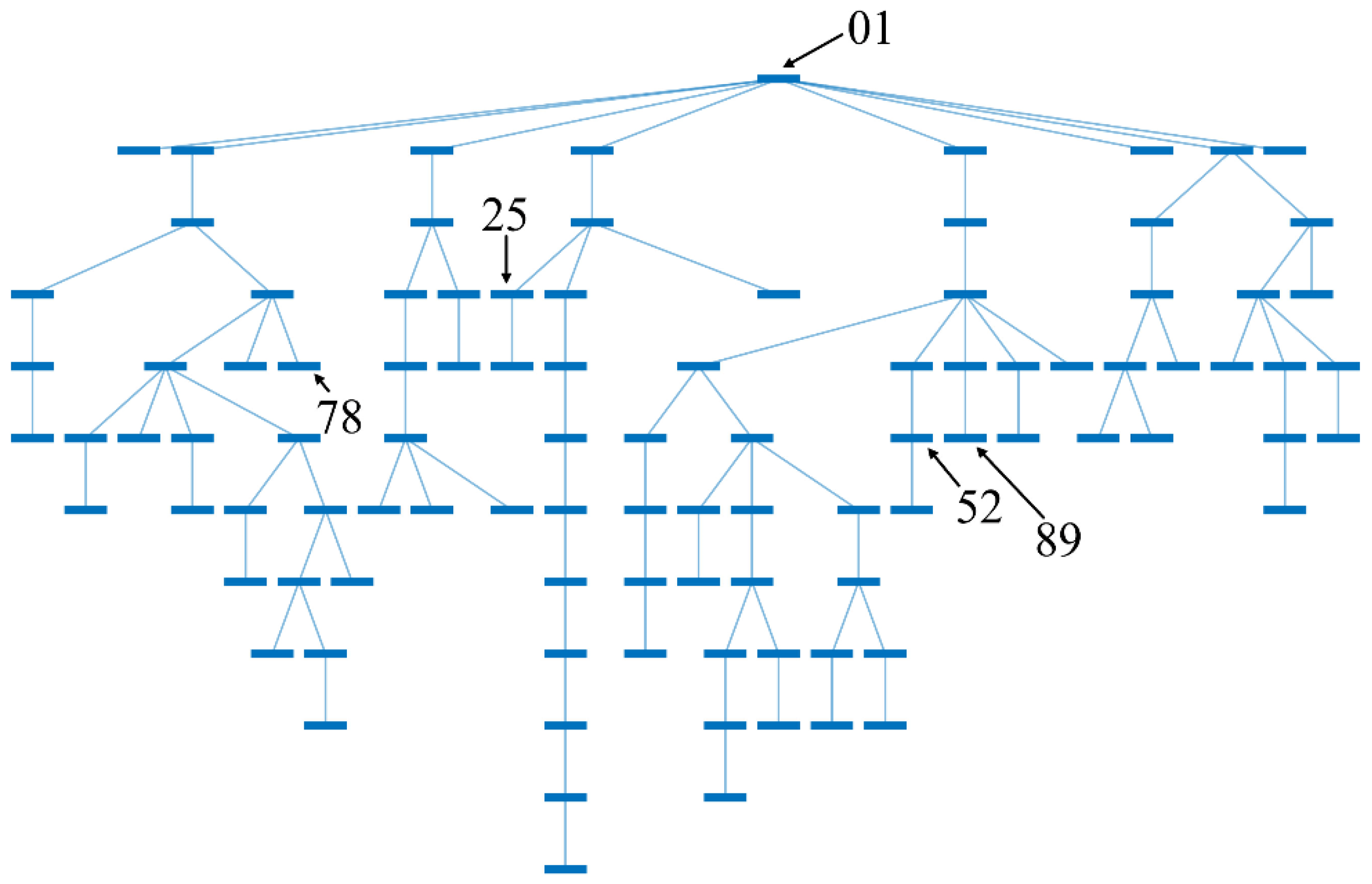
The considered LV network consists of eight longer radial feeders, five of which supply a greater number of customers. The network is composed of underground cables, and the combined length of all main feeders is approximately 6.5 km. It consists of 99 buses and supplies 68 households, where the majority are connected by a three-phase connection. A single-line diagram of the modelled LV network is shown in Figure 1.
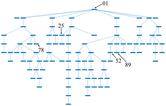
Figure 1.
Simulated network topology.
Bus 01 is the MV/LV transformer secondary bus, and buses 78, 25, 52, and 89 are the voltage measurement buses. Voltage measurements are available from these buses only. At other buses in the network, only the active and reactive injections are available. Measurements are gathered in 10-second intervals. Consequently, the simulation step is also the same.
4.2. Measurements Errors in the Observed Network
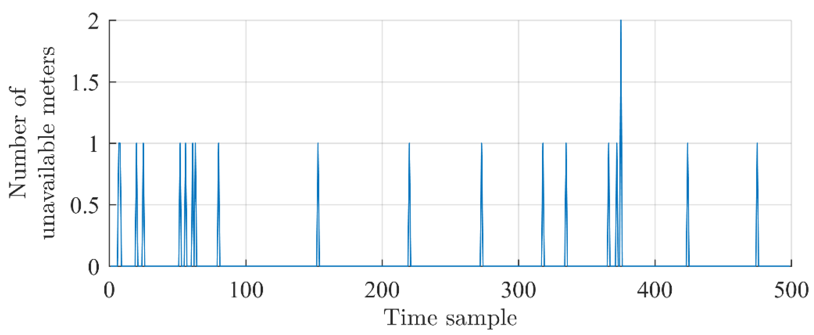
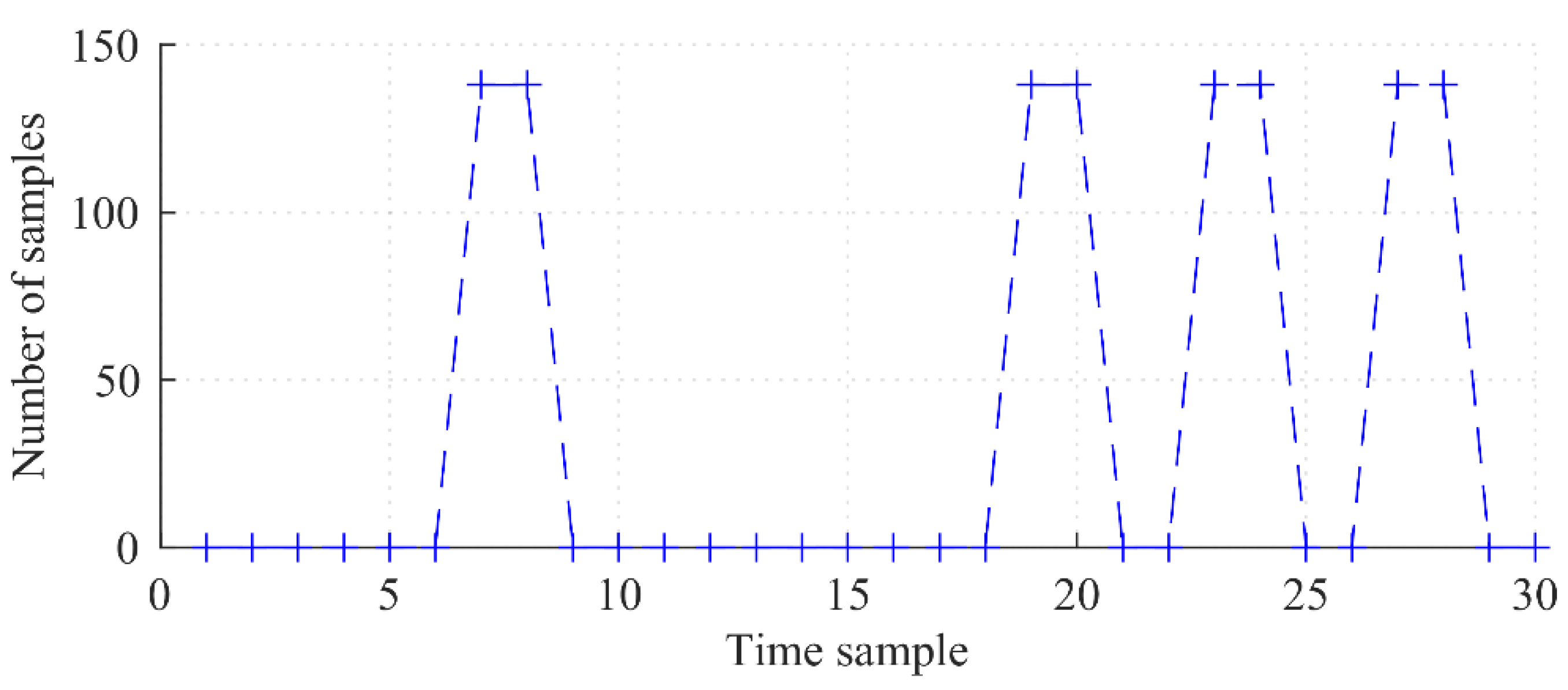
Based on our observations from the real network, spurious measurement errors are a frequent phenomenon. A particular measurement error usually persists for a few consecutive time steps only. To support this notion, a meter unavailability profile for 500 consecutive time steps is presented in Figure 2. Measurement data is collected from meters installed in the observed LV network with a 10-s resolution. As shown, there are missing or erroneous values every now and then at one or two meters. With 10 installed meters, this means that between and of them occasionally fail. A similar success rate was also achieved in the MV network of the pilot, with about 60 m installed. Clearly, measurement intermittence has a negative effect on the estimation process. Thus, for a state estimator to be reliable, a proper method is crucial to overcome, or at least minimize, this issue.
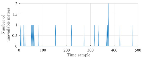
Figure 2.
Network meter unavailability vs. time.
4.3. Network Simulations
For simulations, the OpenDSS [24] software, in conjunction with MATLAB R2016b, was used. OpenDSS is an open source code software tool originally developed by Electrotek Concepts in 1997, and later acquired by the Electric Power Research Institute (EPRI), Palo Alto, CA, USA. It is designed to support distributed energy resource (DER) grid integration and grid modernization. MATLAB® is computing environment for engineers and scientists developed by The MathWorks, Inc., Natick, MA, US.
All network elements, such as lines, busses, loads, and transformers are implemented in OpenDSS. The network element parameters were extracted from the geographic information system (GIS) database provided by the DSO. Load power injections are generated from the database of real measurements. Network measurements (powers and voltages) were extracted from the OpenDSS network simulation.
The network is modelled in full, i.e., all three phase conductors and a neutral conductor are modelled separately. Such an approach is required to take into account phase load imbalance, which is one of significant characteristics of LV networks. The developed state estimator then uses particular measurements in a per-phase manner.
5. Simulation Results
In this section, the simulation results are presented. Four different test cases are considered.
Case 1—Model validation. In this simulation case, the voltages from the simulation environment, which are considered true values, are compared with the estimated values from robust LVSE and WLS estimators in order to prove the validity of the network model.
Case 2—Base case. Here, both algorithms (WLS and the proposed robust LVSE) use measurements that are additionally subjected to a random Gaussian noise. The purpose of this case is to show the superiority of the developed robust LVSE method over the classical WLS in terms of algorithm execution time.
Case 3—Intermittent measurements. In this case, all measurements are subjected to a white Gausssian noise, as in case 2. Additionally, some measurements are substituted with significant errors. The purpose of case 3 is to demonstrate the capability of the robust LVSE method to cope with bad data detection and identification in the case of a state estimation of a poorly-observable network.
Case 4—EV charging. In this case, all measurements are subjected to a white Gausssian noise as in case 2 and case 3. Additionally, two intervals of EV charging are simulated. We have simulated the simultaneous charging of 10 EVs, which results in high load variation in a single time step. The purpose of case 4 is to demonstrate the capability of the robust LVSE method to cope with sudden and unbalanced changes in the demands of the network.
5.1. Case 1: Model Validation
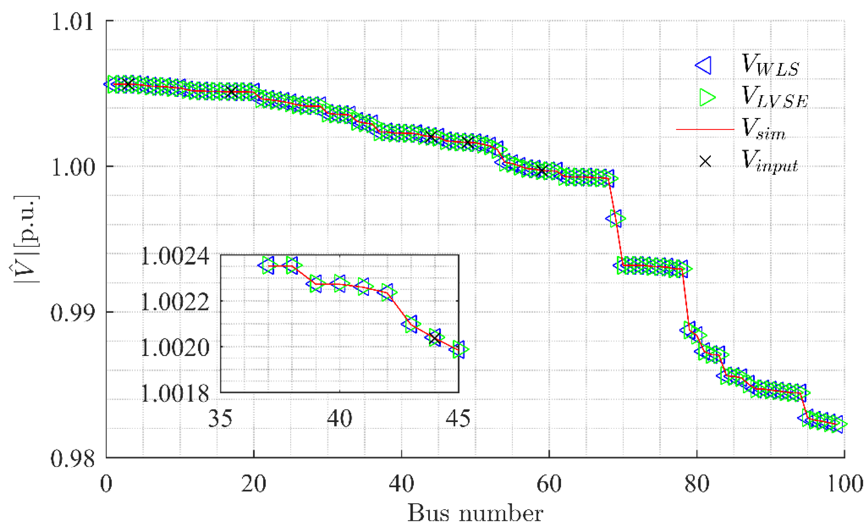
In order to validate the method and the network model included in the algorithm through the matrix, we first simulated the network using the injections and voltages from the OpenDSS simulation model only, i.e., the true values without any additional noise. The network voltage profile is shown in Figure 3. One can see, that both the WLS and robust LVSE estimated profiles follow the simulated voltage, suggesting that the algorithms provide a valid result. The IEKF algorithm was used for robust LVSE algorithm simulation, and both algorithms converged in two iterations per time step.
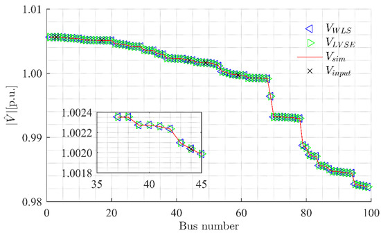
Figure 3.
Network voltage profile—case 1.
5.2. Case 2: Base Case
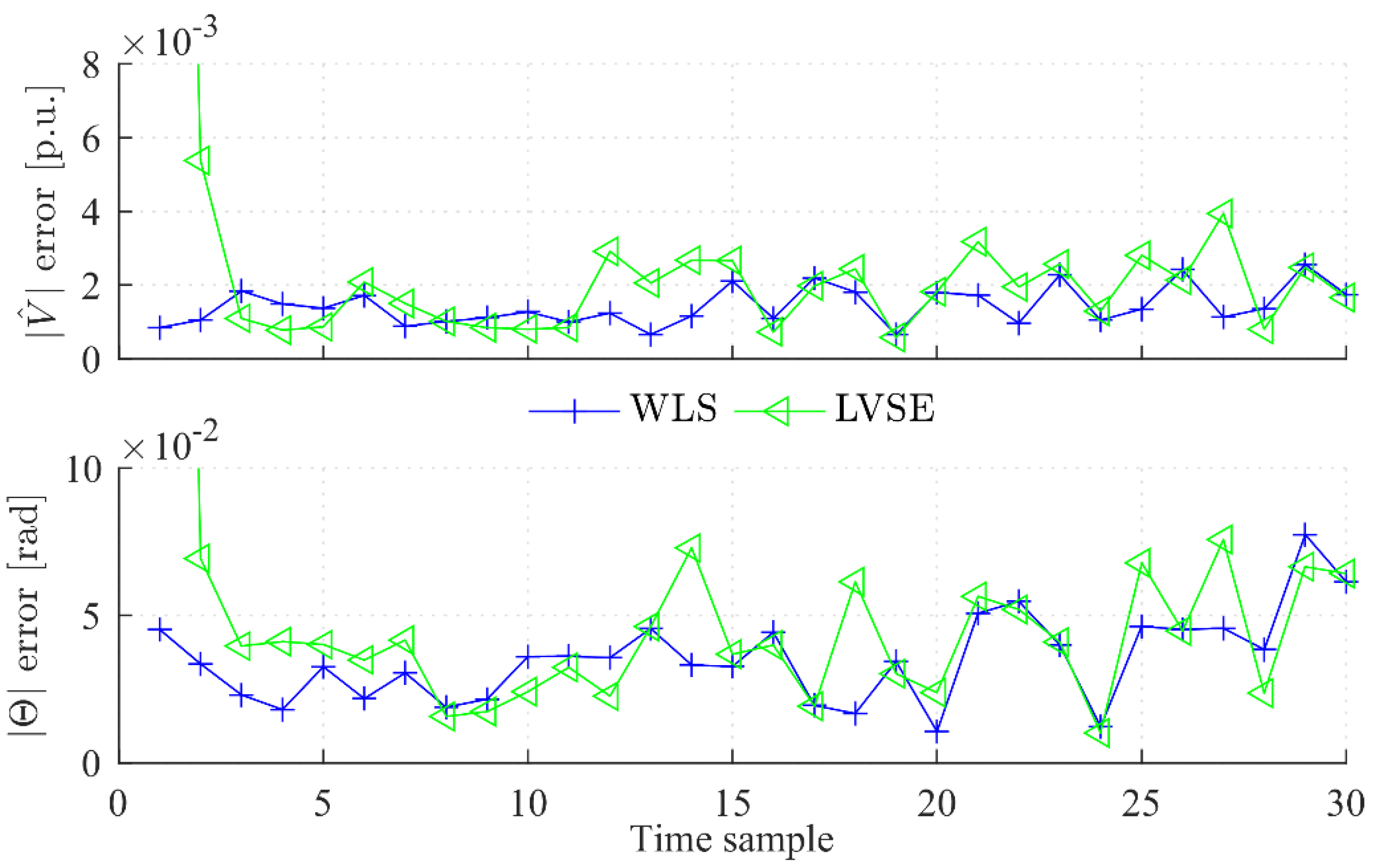
The purpose of this base case is to prove the applicability of the developed robust LVSE method for use in a LV state estimation process. First, the results from a network estimation of a WLS and the developed robust LVSE estimators are presented for the complete set of measurements. The “complete” stands for all power injections at all busses and voltage amplitude measurements at five nodes. In comparison to case 1, each power measurement was subjected to a Gaussian noise of of its true value, and the voltage measurements were modified with a noise of of their true value. The WLS algorithm tolerance was set to , and it converged with two iterations per time step. The robust LVSE performed one iteration only.
The results, in terms of estimate errors and computation time for the estimation of 30 consecutive time steps, are presented below. The maximal deviation for all three phases of voltage amplitudes (absolute values, in p.u.) and of angles (in rad) is shown in Figure 4. One can see that errors of both estimators are similar for the same time steps. A higher error in the first two steps can be observed in the case of the robust LVSE algorithm, since it needs a few iterations for its initialization.
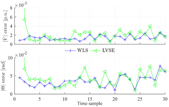
Figure 4.
Estimation error—case 2.
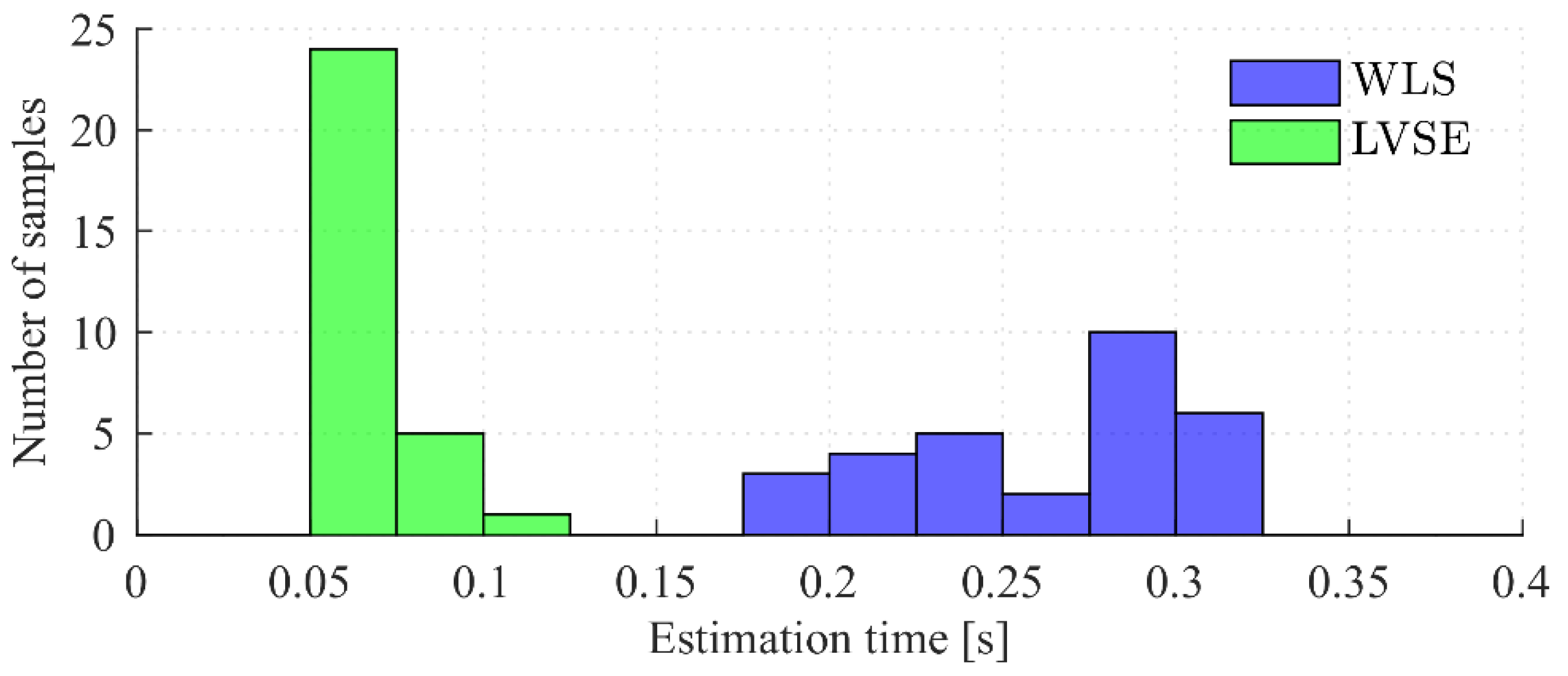
The results in terms of calculation duration are shown in Figure 5. As shown, robust LVSE is faster, with a median step-calculation duration of 0.07 s. One step-calculation stands for a calculation of estimates for all 3 phases. The median step-calculation duration of the WLS algorithm is 0.28 s. The base case results show that the robust LVSE algorithm is considerably faster when compared to the WLS, while the accuracy of both algorithms is similar.
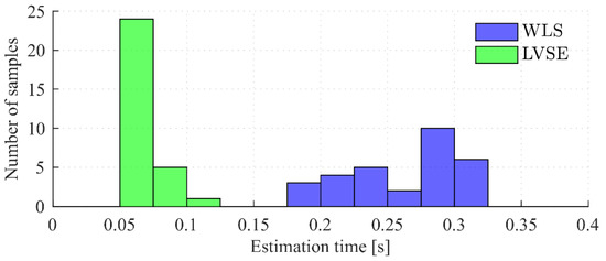
Figure 5.
Estimation duration distributions—case 2.
5.3. Case 3: Intermittent Measurements
Based on our experience during field testing, the real distribution network measurements are highly intermittent (as shown in Figure 2). Namely, the metered values are not successfully transmitted to the SCADA/DMS system for different reasons, such as the temporary failure of a meter, or more often, issues with the communication infrastructure. A particular measurement can thus be delayed, corrupted, or even lost [25]. Due to a variety of interferences, there are also measurements with spikes of positive and negative magnitudes. These spikes must be filtered by the estimation algorithm, otherwise the estimates are wrong.
The measurement set used for the case 2 simulation is already critical, and the removal of any of the measurements from the set makes it critical (lost redundancy). Redundancy is one of the key factors in the estimation process, and in the case of a non-redundant measurement set, estimation is not possible [14].
In case 3 (intermittent measurements case), the same network is simulated as in case 2, and we are using the same estimators as before. Additionally, these are the operating conditions in case 3:
- Bad data: measurements of both active and reactive power injections at buses 24, 37, 72, and 76 are multiplied by a factor of 100 before entering the SE in order to simulate erroneous peaks in the incoming measurements. Buses were randomly chosen among the buses with connected loads.
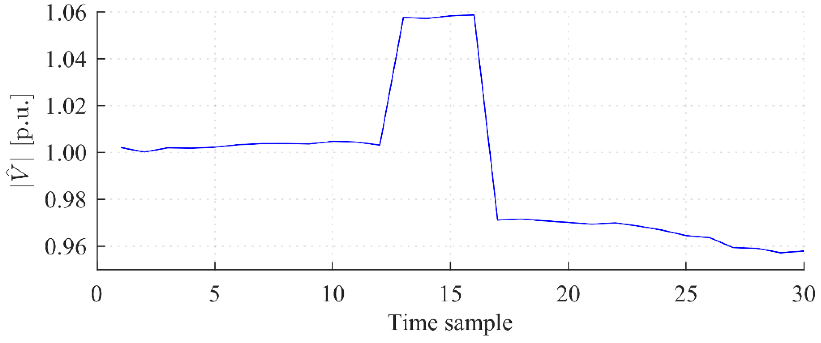
- Voltage change: HV/MV transformer OLTC tap was changed in order to rapidly change the secondary busbar voltage, and consequently, all the voltages in the LV network. In the case of a voltage increase before the time instant 13, the sending busbar voltage was changed from 1.0 p.u. to 1.06 p.u. Then, before time instant 17, this voltage was lowered to 0.97 p.u. The MV/LV transformer sending the busbar voltage for the considered time instants is shown in Figure 6. The voltages of all three phases are quite symmetrical at the supply point of the LV network, and thus, only the mean value is shown. One can also notice additional voltage variations due to changes of the loading at different time instants.
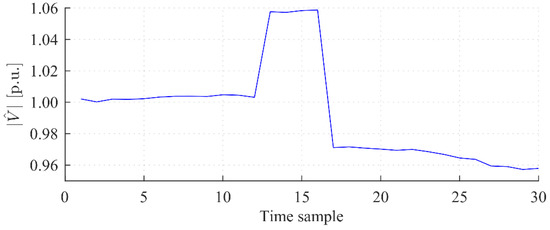 Figure 6. MV/LV transformer secondary busbar voltage (mean)—case 3.
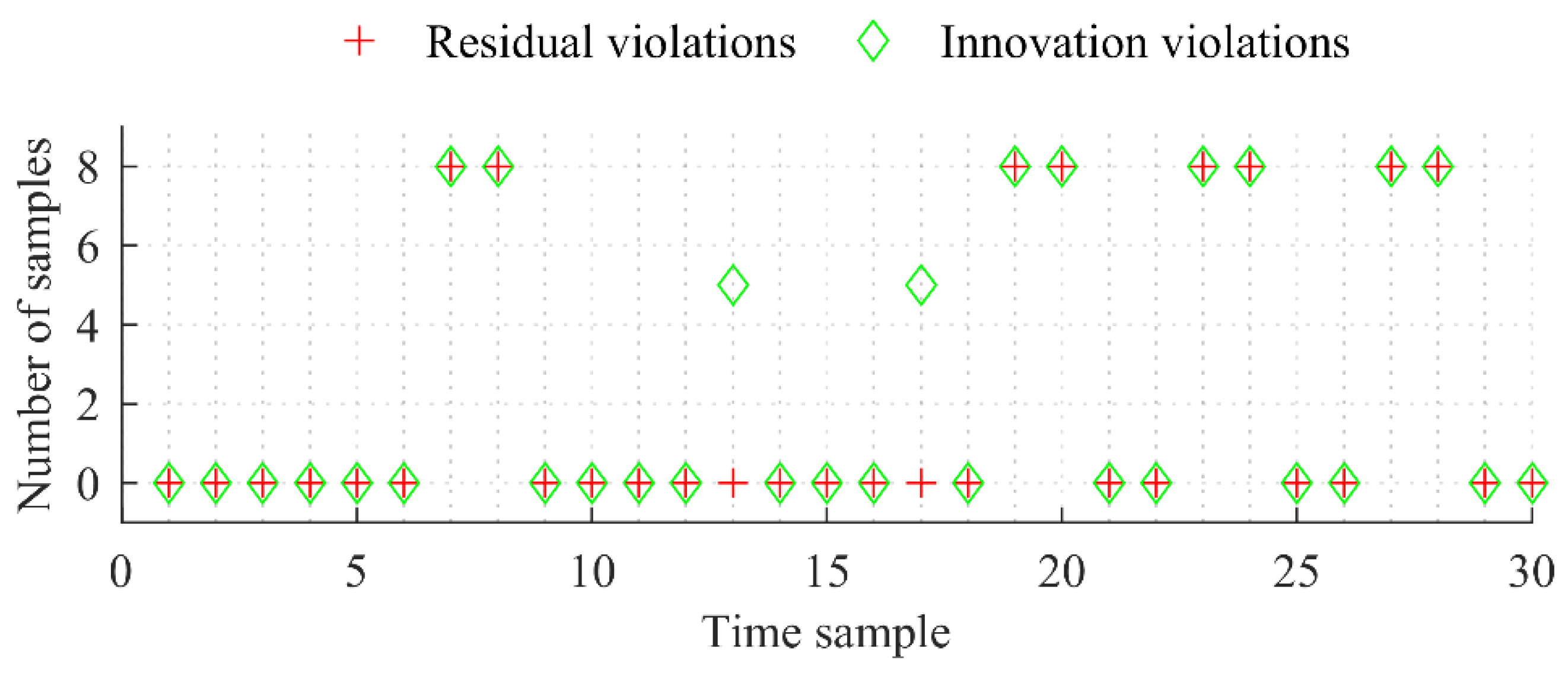
A classical WLS estimator detected the error in the measurement set. However, due to the low redundancy, it was not able to identify the erroneous measurement locations with simultaneous errors at four different busses (P and Q measurements). Therefore, its output is not useful in this case, since all received measurements, besides the voltages, were flagged as erroneous, as shown in Figure 7.
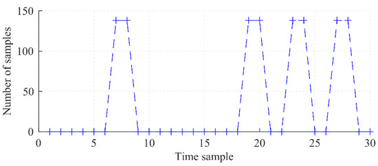
Figure 7.
WLS measurement error flags—case 3.
On the other hand, the introduced erroneous measurements were correctly detected by the robust LVSE algorithm, and their locations were identified by the estimator in the process of innovation analysis. The detected errors are flagged, as shown in Figure 8. Instead of the identified erroneous measurements, their a priori predictions are used in the latter filtering process, and consequently, the estimation process converges. Estimation errors in this case are larger, since the predictions are not as good as true measurements. Only flags for one phase are presented, since the errors are symmetrical for each phase and, consequently, so are the threshold violation flags. From Figure 8 it can be also seen that in case of a sudden voltage change in the network, there are no residual-violation flags set. Instead, only five innovations are flagged as errors. These are voltage measurements from the measurement set, which do not follow the previous trend as a consequence of the OLTC manipulation.
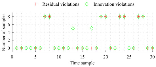
Figure 8.
Robust LVSE measurement error flags—case 3.
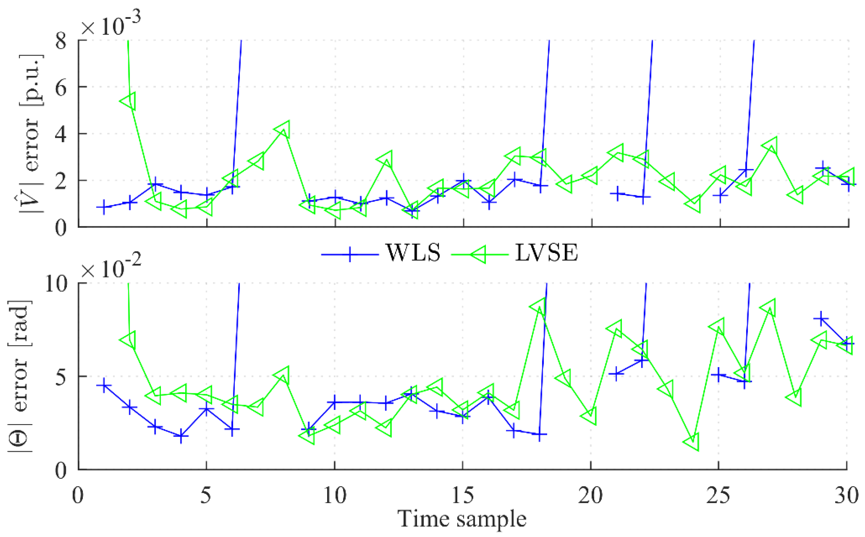
The accuracy of the estimation results for each of the considered 30 consecutive steps, in terms of maximal amplitude and angle deviation (all 3 phases), is shown in Figure 9.
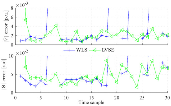
Figure 9.
Estimation error—case 3.
On average, WLS estimation performs a bit better when all of the measurements in the measurement set are OK. In case of simultaneous bad data, the robust LVSE algorithm outperforms the WLS, since WLS diverges due an unobservable network.
Besides the accuracy of the calculated estimates, also the duration of the estimation process is of importance. Estimation times for the considered time interval are shown in Figure 10. As shown, robust LVSE has a median step-calculation time (all 3 phases) of 0.07 s, which is considerably faster than the WLS algorithm median step-calculation time of 0.27 s. Note that only iterations in which the WLS algorithm converged were used for the WLS median calculation. There are, however, two time instants in which the robust LVSE calculation time was longer. These are the two samples in which a sudden change occurred and, consequently, the LVSE was iteratively repeated until the preset tolerance value.
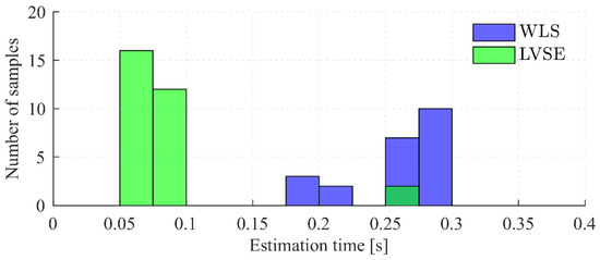
Figure 10.
Estimation duration distributions—case 3.
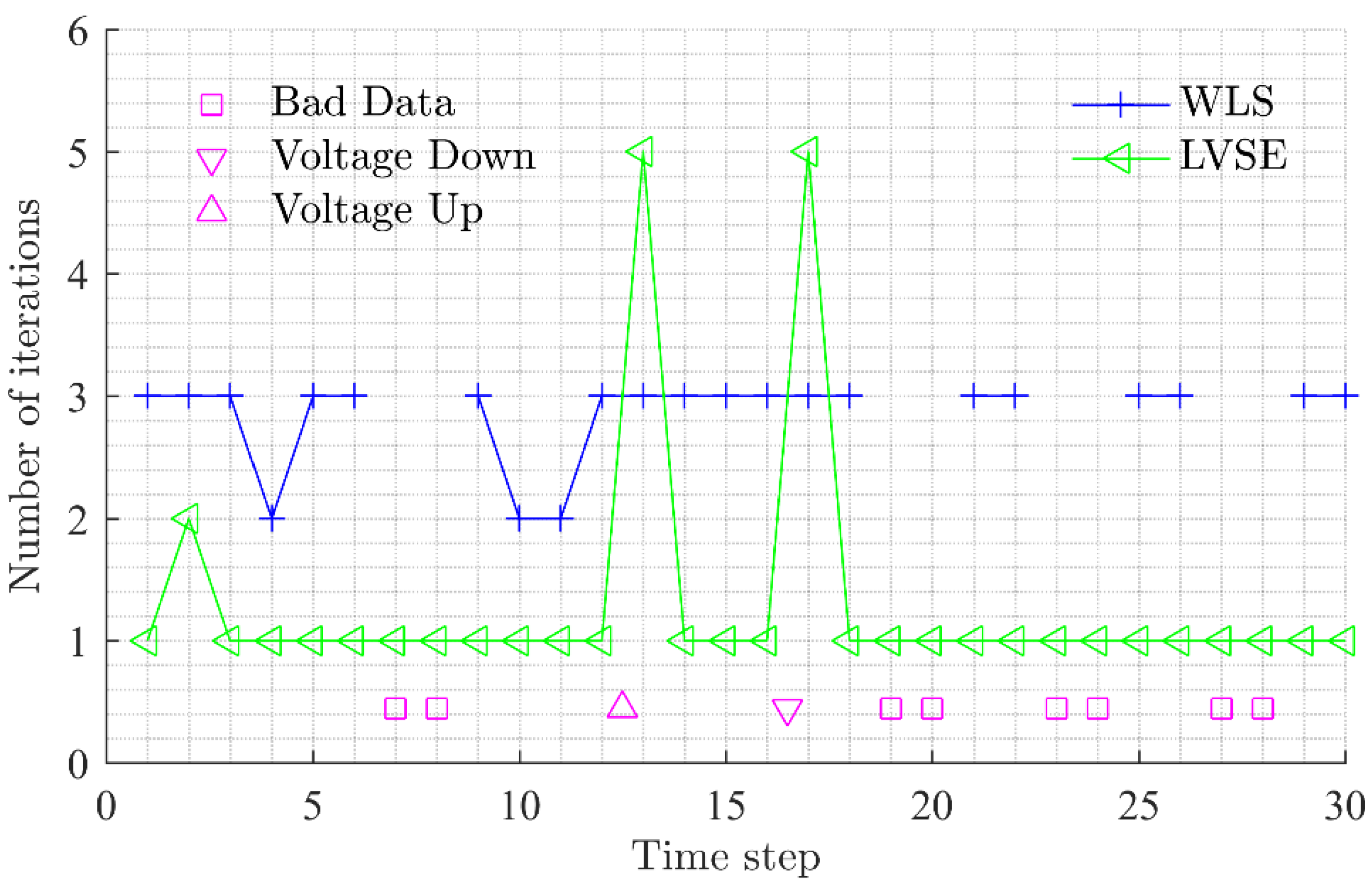
The algorithm efficiency in terms of the number of iterations per calculation step is shown in Figure 11. For the WLS algorithm, only the time instants where the algorithm converged are displayed. The type of imposed measurement anomaly is presented in the same figure. From the figure, it can be seen that the number of WLS iterations is larger than the number of robust LVSE iterations for all time instants, with the exception of instants with OLTC operation. In case of a sudden change and in time step 2, the robust LVSE is iteratively repeated in order to converge to a solution.
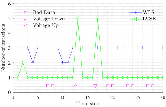
Figure 11.
Number of iterations per step.
5.4. Case 4: EV Charging
Due to the high penetration of various loads with a high nominal power, such as EVs, battery storage, and distributed generation, the distribution network is subjected to continuous and sometimes unpredictable changes in demand. The developed SE algorithm must be capable of providing accurate estimates of the network state despite abrupt consumption changes.
Case 4 shows the results of the network estimation for the case of high EV penetration. There are 10 EVs in the network, randomly allocated to 10 LV network customers. It is assumed that each of the EVs is being charged through a single-phase domestic charger with nominal power of 3.7 kW. The phase allocation for each of the 10 EVs was random, resulting in 5 EVs connected to phase A, 4 to phase C, and 1 to phase B, as presented in Table 2.
Table 2.
EV connection by phase.
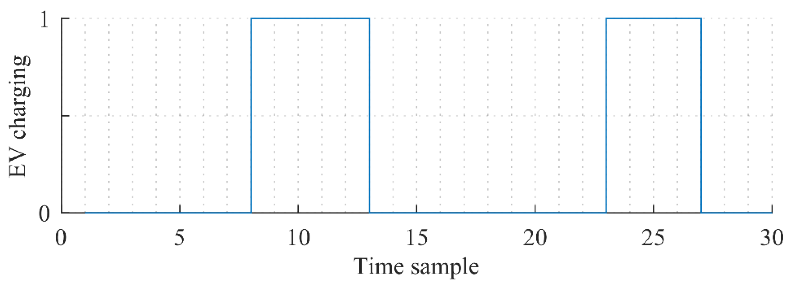
A worst-case scenario was assumed for the simulation, where all 10 EVs started and stopped charging at the same time. Consequently, the load deviation in the network was high. Since the purpose of this case is to test the ability of the developed LVSE to withstand higher load changes, two charging intervals were simulated in the period of 30 consequent time samples, with a resolution of 10 s. In terms of real EV charging, the charging interval would have been longer. However, as mentioned before, the robustness of the developed LVSE is tested here, rather than the actual charging process. The active charging profile is demonstrated in Figure 12. As shown, the EVs are being charged in intervals 8–12 and 23–26.
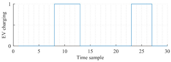
Figure 12.
EV charging profile—case 4.
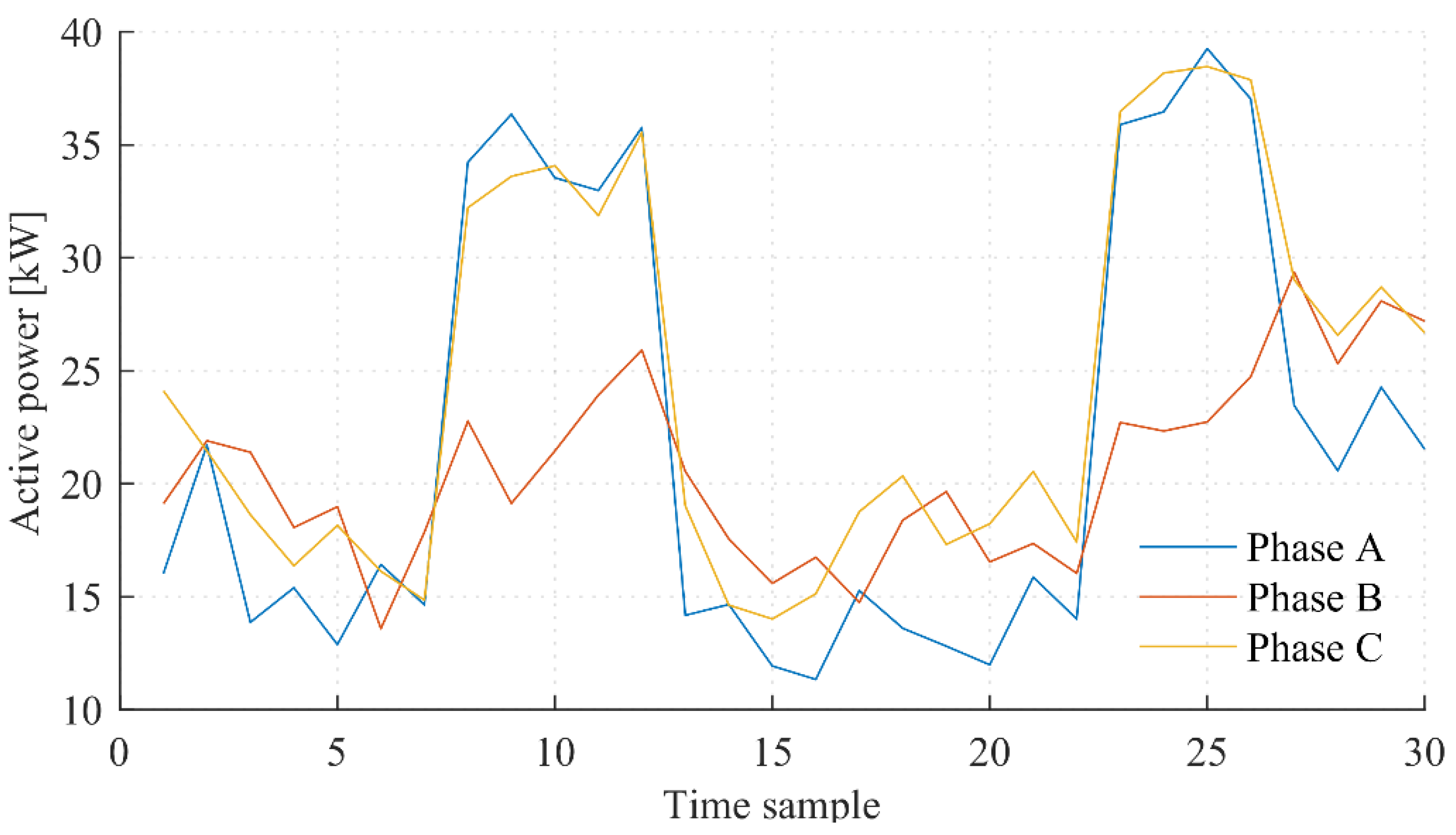
The network consumption in terms of active power flow through the supplying MV/LV transformer is shown in Figure 13. Phases A and C exhibit a significant peak during the EV charging intervals, while this is not significant in phase B, since only one EV is supplied through phase B.
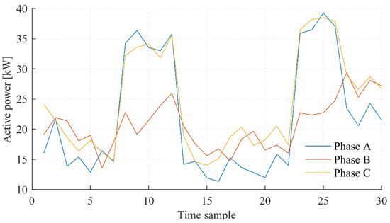
Figure 13.
Network consumption—active power—case 4.
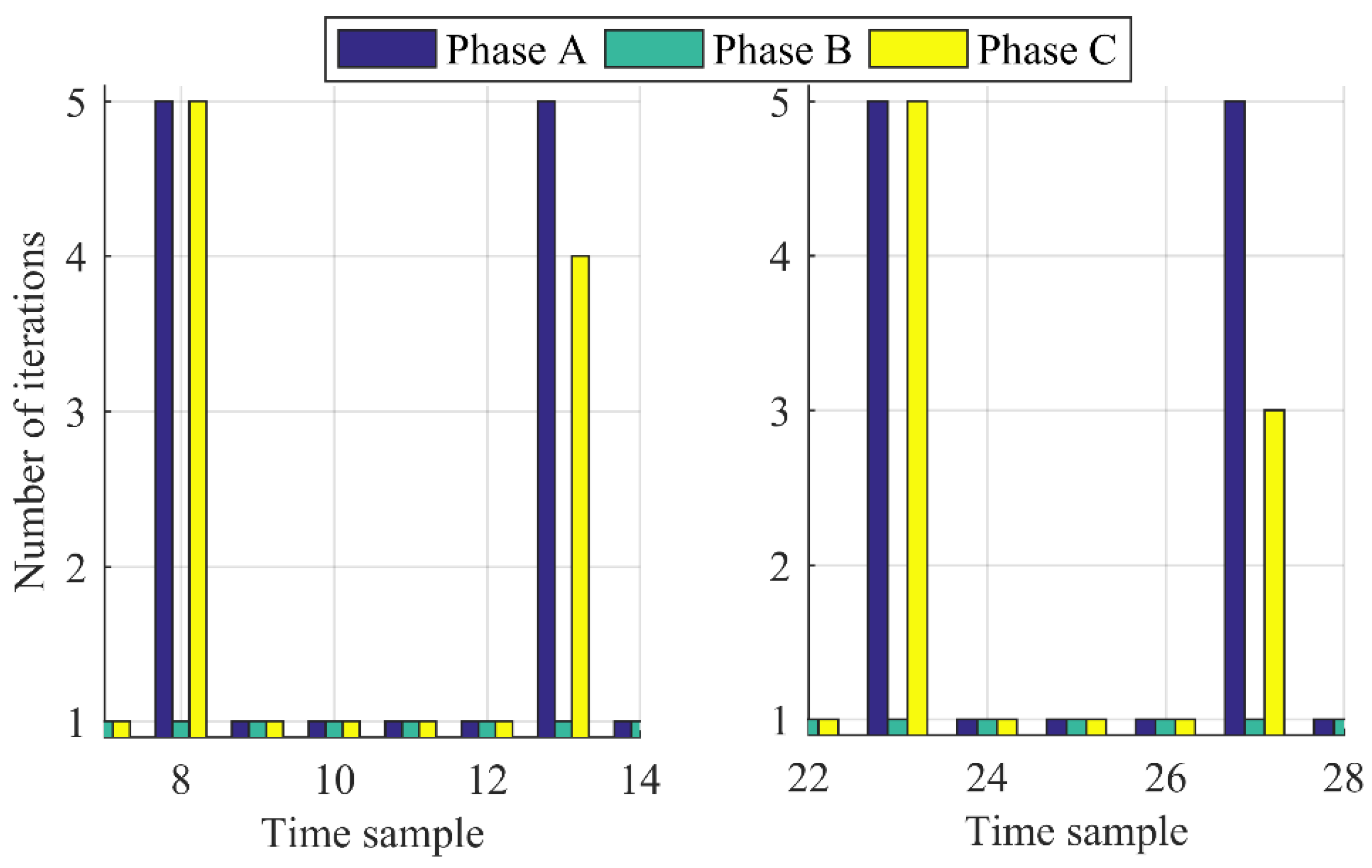
The developed LVSE algorithm correctly identified a sudden change in the network consumption levels. What is more, the change was detected on phases A and C, while the phase B demand variation was too low to be identified. Because of the identified network change, the algorithm was re-initialized for the phases, which experienced the change of demand. The number of algorithm iterations, for each phase, is presented in Figure 14.

Figure 14.
Number of algorithm iterations—case 4.
As shown, the algorithm always converges in one iteration in the case of phase B estimation, while it is re-iterated at the time instants of demand change for the other two phases. In case of re-initialization, the number of iterations is repeated until the difference between the consecutive estimates falls below the predefined tolerance value.
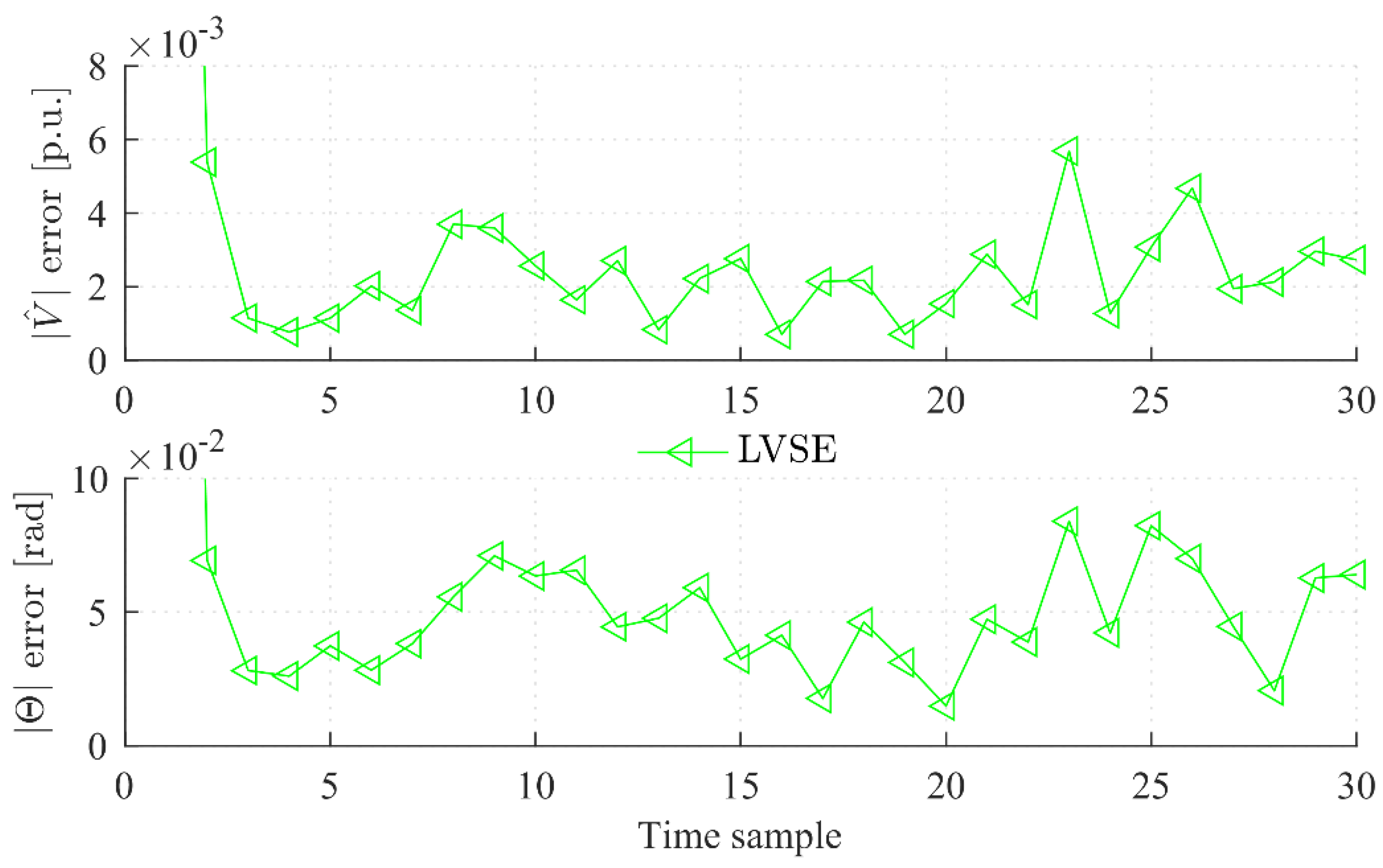
The accuracy of the estimation results for each of the considered 30 consecutive steps, in terms of maximal amplitude and angle deviation (all 3 phases), is shown in Figure 15. The error remains within similar margins as those in both previous cases (shown in Figure 4 and Figure 9). The results of case 4 demonstrate the ability of the proposed algorithm to identify and withstand an unbalanced change in the network.
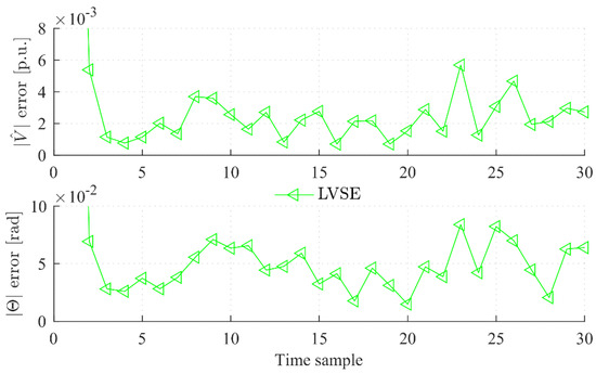
Figure 15.
Estimation error—case 4.
6. Conclusions
This paper presented a novel approach for state estimations of poorly-monitored low-voltage networks with unreliable measurements, focusing on estimation speed and algorithm robustness.
A Kalman filter-based robust LVSE algorithm with a modification of the filtering process was used. Namely, we used constant Kalman gain and Jacobian matrices that were changed only after a larger disturbance had occurred in the network. This approach considerably reduced the duration of the calculation while preserving the accuracy of the estimates.
The simulations showed that the developed robust LVSE method outperforms the classical WLS algorithm in terms of calculation durations and algorithm robustness. Its superiority is especially noticeable in cases of measurements intermittence, which is a common issue in low-voltage network measurements. The robust LVSE method was able to withstand the simulated meter failures and still provide accurate estimates. The results also demonstrate that the developed LVSE method is able to cope with highly unbalanced changes of consumption. The latter are expected to occur frequently in the future, as a result of a gradually increasing share of EVs on the network.
The presented robust LVSE estimator is planned for implementation in an online distribution network state-estimation process as part of an advanced voltage control functionality. Field tests will probably yield some additional challenges, which will be addressed in the scope of the future work.
Author Contributions
Conceptualization, M.A. and B.B.; Data curation, M.A.; Investigation, M.A.; Methodology, B.B.; Project administration, I.P. and B.B.; Software, M.A.; Supervision, B.B.; Validation, B.B.; Visualization, M.A.; Writing—original draft, M.A.; Writing—review & editing, M.A., I.P. and B.B.
Funding
This research was funded by Slovenian Research Agency with the young researchers funding mechanism.
Conflicts of Interest
The authors declare no conflict of interest.
References
- Hayes, B.; Prodanovic, M. State estimation techniques for electric power distribution systems. In Proceedings of the 2014 IEEE European Modelling Symposium (EMS), Pisa, Italy, 21–23 October 2014; pp. 303–308. [Google Scholar]
- da Silva, A.M.L.; Filho, M.B.D.C.; De Queiroz, J.F. State forecasting in electric power systems. Transm. Distrib. IEE Proc. C—Gener. 1983, 130, 237–244. [Google Scholar] [CrossRef]
- da Silva, A.M.L.; Filho, M.B.D.C.; Cantera, J.M.C. An Efficient Dynamic State Estimation Algorithm including Bad Data Processing. IEEE Trans. Power Syst. 1987, 2, 1050–1058. [Google Scholar] [CrossRef]
- Filho, M.B.D.C.; de Souza, J.C.S. Forecasting-Aided State Estimation—Part I: Panorama. IEEE Trans. Power Syst. 2009, 24, 1667–1677. [Google Scholar] [CrossRef]
- Filho, M.B.D.C.; de Souza, J.C.S.; Freund, R.S. Forecasting-Aided State Estimation #x2014; Part II: Implementation. IEEE Trans. Power Syst. 2009, 24, 1678–1685. [Google Scholar]
- Lu, Z.; Yang, S.; Sun, Y. Application of extended fractional Kalman filter to power system dynamic state estimation. In Proceedings of the 2016 IEEE PES Asia-Pacific Power and Energy Engineering Conference (APPEEC), Xi’an, China, 25–28 October 2016; pp. 1923–1927. [Google Scholar]
- Saikia, A.; Mehta, R.K. Power system static state estimation using Kalman filter algorithm. Int. J. Simul. Multisci. Des. Optim. 2016, 7, A7. [Google Scholar] [CrossRef]
- Blood, E.A.; Krogh, B.H.; Ilic, M.D. Electric power system static state estimation through Kalman filtering and load forecasting. In Proceedings of the 2008 IEEE Power and Energy Society General Meeting—Conversion and Delivery of Electrical Energy in the 21st Century, Pittsburgh, PA, USA, 20–24 July 2008; pp. 1–6. [Google Scholar]
- Abdel-Majeed, A.; Braun, M. Low voltage system state estimation using smart meters. In Proceedings of the 2012 47th International Universities Power Engineering Conference (UPEC), London, UK, 4–7 September 2012; pp. 1–6. [Google Scholar]
- Abdel-Majeed, A.; Tenbohlen, S.; Rudion, K. Effects of state estimation accuracy on the voltage control of low voltage grids. In Proceedings of the 2015 International Symposium on Smart Electric Distribution Systems and Technologies (EDST), Vienna, Austria, 8–11 September 2015; pp. 526–530. [Google Scholar]
- Waeresch, D.; Brandalik, R.; Wellssow, W.H.; Jordan, J.; Bischler, R.; Schneider, N. Linear state estimation in low voltage grids based on smart meter data. In Proceedings of the 2015 IEEE Eindhoven PowerTech, Eindhoven, The Netherlands, 29 June–2 July 2015; pp. 1–6. [Google Scholar]
- Nishiya, K.; Hasegawa, J.; Koike, T. Dynamic state estimation including anomaly detection and identification for power systems. Transm. Distrib. IEE Proc. C—Gener. 1982, 129, 192–198. [Google Scholar] [CrossRef]
- Hajiyani, P.; Lev-Ari, H.; Stanković, A.M. Mitigating bad data and measurement delay in nonlinear dynamic state estimation. In Proceedings of the 2016 IEEE International Symposium on Circuits and Systems (ISCAS), Montreal, QC, Canada, 22–25 May 2016; pp. 678–681. [Google Scholar]
- Filho, M.B.D.C.; de Souza, J.C.S.; de Oliveira, F.M.F.; Schilling, M.T. Identifying critical measurements amp; sets for power system state estimation. In Proceedings of the 2001 IEEE Porto Power Tech Proceedings (Cat. No.01EX502), Porto, Portugal, 10–13 September 2001; Volume 3, p. 6. [Google Scholar]
- Do Coutto Filho, M.B.; Souza, J.C.S.; Matos, R.S.G.; Schilling, M.T. Revealing gross errors in critical measurements and sets via forecasting-aided state estimators. Electr. Power Syst. Res. 2001, 57, 25–32. [Google Scholar] [CrossRef]
- Abur, A.; Exposito, A.G. Power System State Estimation: Theory and Implementation; CRC Press: Boca Raton, FL, USA, 2004. [Google Scholar]
- Kuhar, U.; Pantoš, M.; Kosec, G.; Švigelj, A. The Impact of Model and Measurement Uncertainties on a State Estimation in Three-Phase Distribution Networks. IEEE Trans. Smart Grid 2018, 10, 3301–3310. [Google Scholar] [CrossRef]
- Antončič, M.; Blažič, B. LV Network State Estimation Using Decoupled Load-Flow Algorithm. In Proceedings of the CIRED Workshop, Ljubljana, Slovenia, 7–8 June 2018; Volume 2018, p. 4. [Google Scholar]
- Schweppe, F.C.; Wildes, J. Power System Static-State Estimation, Part I: Exact Model. IEEE Trans. Power Appar. Syst. 1970, PAS–89, 120–125. [Google Scholar] [CrossRef]
- Monticelli, A. State Estimation in Electric Power Systems; Springer: Boston, MA, USA, 1999; ISBN 978-1-4613-7270-7. [Google Scholar]
- Kalman, R.E. A new approach to linear filtering and prediction problems. J. Basic Eng. 1960, 82, 35–45. [Google Scholar] [CrossRef]
- Grewal, M.S.; Andrews, A.P. Applications of Kalman Filtering in Aerospace 1960 to the Present [Historical Perspectives]. IEEE Control Syst. 2010, 30, 69–78. [Google Scholar] [CrossRef]
- Ljung, L. Asymptotic behavior of the extended Kalman filter as a parameter estimator for linear systems. IEEE Trans. Autom. Control 1979, 24, 36–50. [Google Scholar] [CrossRef]
- Electric Power Research Institute. OpenDSS Manual; Electric Power Research Institute: Palo Alto, CA, USA, 2010. [Google Scholar]
- Jin, Z.; Ko, C.; Murray, R.M. Estimation for Nonlinear Dynamical Systems over Packet-Dropping Networks. In Proceedings of the 2007 American Control Conference, New York, NY, USA, 9–13 July 2007; pp. 5037–5042. [Google Scholar]

© 2019 by the authors. Licensee MDPI, Basel, Switzerland. This article is an open access article distributed under the terms and conditions of the Creative Commons Attribution (CC BY) license (http://creativecommons.org/licenses/by/4.0/).