An Improved Bare Bone Multi-Objective Particle Swarm Optimization Algorithm for Solar Thermal Power Plants

Abstract

Solar energy has many advantages, such as being abundant, clean and environmentally friendly. Solar power generation has been widely deployed worldwide as an important form of renewable energy. The solar thermal power generation is one of a few popular forms to utilize solar energy, yet its modelling is a complicated problem. In this paper, an improved bare bone multi-objective particle swarm optimization algorithm (IBBMOPSO) is proposed based on the bare bone multi-objective particle swarm optimization algorithm (BBMOPSO). The algorithm is first tested on a set of benchmark problems, confirming its efficacy and the convergency speed. Then, it is applied to optimize two typical solar power generation systems including the solar Stirling power generation and the solar Brayton power generation; the results show that the proposed algorithm outperforms other algorithms for multi-objective optimization problems.

1. Introduction

The energy issue is viewed as one of many global problems in the 21st century and it is projected that the global energy demand will increase by almost a quarter by 2040 [1]. The continuous rise of prices for fossil fuels and the climate change due to substantive consumption of non-renewable energies have caused the shift of energy landscape, from the way the energy is sourced to the way energy is consumed. The landscape change of the energy mix is also largely due to more strict legislations on pollutant and green-gas-house emissions and policies to encourage the use of renewable sources. For example, the European Union requires all its members to take a series of measures to improve energy efficiency of at least 20% [2]. In addition to this initiative, the United Nations General Assembly declared the decade 2014–2024 as the “Decade of Sustainable Energy for All”, given the importance of energy issues for sustainable development [3] and encouraging and supporting the extended use of renewable energy resources (RES).

As an ideal renewable energy source, solar energy is one of the most abundant energy resources. Solar power has many advantages such as being clean, renewable, and easy to store [4]. Solar power can be used to generate electricity wherever there is sunshine. Therefore, in the context of the growing global energy demand and increasing concerns relating to resources, environment and climate, governments worldwide have developed a range of policies and incentive mechanisms to promote the development and roll-out of renewable generation technologies for solar and wind energy sources [5].

Solar thermal power generation technology is a relatively mature technology which mainly uses the solar concentrating system to convert the solar energy to a high temperature steam and then drives the generators to generate electricity [6]. Representative solar thermal power generation systems include a solar Stirling cycle power generation system and a solar Brayton cycle power generation system.

In the 1970s, research on dish solar Stirling power generation technology was initiated by MDAC, NASA and USAB. The early solar Stirling power generation system was mainly composed of solar concentrating mirrors, tubular illuminating collectors, heat engines and so on [7]. In 2005, the first 10 kW dish-type solar Stirling generator system was built at the CNRS-PROMES laboratory in Odeillo, and details of the system are given in [8]. Afterwards, Hafez et al. [9] presented parameter design, simulation experiments and thermodynamic analysis on the dish solar Stirling generator system, which provided theoretical guidance for the design and operation of the dish solar power system. Caballero et al. [10] verified a dish Stirling model based on real technical data, and proposed a method to determine the operating temperature of the receiver and optimized the parameters of the dish solar Stirling cycle system. Li et al. [11] proposed a new system control method to achieve the maximum power point tracking and constant receiver temperature of the dish Stirling system.

Solar Brayton power generation technology is another typical solar thermal power technology. Although its thermal energy conversion efficiency is not as high as that of Stirling heat engine, it is more mature in technology. The solar Brayton cycle has higher reliability and broad application prospects because the Brayton cycle structure is simpler, which only needs one transmission component (compressor/generator). Since the 1960s, the United States has taken the lead in solar Brayton power generation research [12]. The Free Space Station study, which began in 1980, further promoted the development of space solar Brayton technology and related theoretical research [13]. Meas et al. [14] studied the effects of heating and cooling on the maximum net output power of open and restored solar Brayton cycles using a method of minimizing the entropy generation. Praveen et al. [15] performed a detailed thermodynamic analysis of the dish solar collector based on the Brayton thermostat cycle and determined the important dimensionless parameters of the coupled system optimization performance. Recently, Khan [16] proposed a new parabolic dish solar collector with cavity receiver, working on three different thermal oil based nanofluids (Al₂O₃, CuO & TiO₂), which is integrated with supercritical carbon dioxide Brayton cycle for power production.

In general, solar power generation systems are complex systems which have to be optimally designed. This paper investigates the modelling of the aforementioned two typical solar power generation systems, namely, solar Stirling cycle power generation system and solar Brayton cycle power generation system. These two systems are highly non-linear, and it is a challenging multi-objective optimization problem to identify a suitable model.

Currently, methods to solve multi-objective optimization problems (MOPs) can be grouped into two categories. The first group includes traditional methods, such as weighted sum methods [17], gain programming [18,19,20] and compromise programming [21,22]. These traditional methods are often highly efficient, however, they are difficult to handle high dimensional complex engineering problems. The other group covers evolutionary algorithms based on the Pareto optimum such as non-dorminated sorting genetic algorithm (NSGA2) [23], multi-objective particle swarm optimization (MOPSO) [24], multi-objective defferential evolution (MODE) [25], and the multi-objective evolutionary algorithm based on decomposition (MODE/A) [26], etc. These algorithms not only have the characteristics of high parallelism, self-organization, self-learning and self-adaptation, but also have no restrictions on the search space therefore overcoming the shortcomings of traditional algorithms.

Computation-based methods have also been used in the study of solar thermal generation systems with multi-objective functions. Mohammad et al. used the NSGA2 algorithm to optimize the dish solar Stirling generator system with maximum power output, maximum entropy generation rate and maximum thermal effici ency and three different multi-objective decision-making methods are used [27]. Li et al. optimized the dish solar Brayton system using the NSGA2 algorithm with the goal of maximizing the power output, the thermal efficiency and the ecological performance [28,29].

Particle swarm optimization (PSO) proposed by Kennedy [30] is inspired by the foraging phenomenon of birds. It has the advantages of being simple to implement and having strong global search ability, therefore can be used to handle a range of MOPs. For example, Tripathi [31] proposed an adaptive MOPSO algorithm that uses inertia weights and learning factors as part of the decision variables. Praveen [32] applied linear decreasing weights and time-varying learning factor strategies to MOPSO, leading to the proposal of a time-varying multi-objective particle swarm optimization algorithm. Based on the single-objective backbone particle swarm optimization algorithm, Zhang [33] proposed a BBMOPSO algorithm with fewer parameters by introducing external file mechanism and congestion strategy. The traditional MOPSO algorithm has the disadvantage of relying heavily on the choice of initial values for the tuning parameters. This paper proposes an IBBMOPSO algorithm which improves the performance of traditional MOPSO algorithm with different mutation mechanisms. The algorithm replaces the Gaussian time-varying variation mechanism in the traditional BBPSO algorithm with a widely varying Cauchy time-varying variation mechanism, thus improving the global searching ability of the algorithm while maintaining the diversity of solutions. To overcome the shortcomings of traditional cross-border processing mechanism used in multi-objective optimization, this paper further proposes an improved cross-border processing mechanism (random perturbation mechanism) to further improve the diversity of solutions.

The rest of the paper is organized as follows. Section 2 mainly introduces the mathematical model of the solar Stirling power generation system and the solar Brayton power generation system. In Section 3, the basic MOPSO algorithm and the IBBMOPSO algorithm is proposed. Section 4 verifies the performance of the proposed algorithm through simulation experiments. Section 5 applies the new algorithm to two different solar power system models.

2. Mathematical Model of Solar Power Generation System

This paper studies two different solar power generation systems, including the solar Stirling cycle power generation system and the solar Brayton cycle power generation system. Modelling of the solar Stirling power generation system is a multi-objective unconstrained optimization problem, while modelling of the solar Brayton power generation system is a continuous optimization constraint problem.

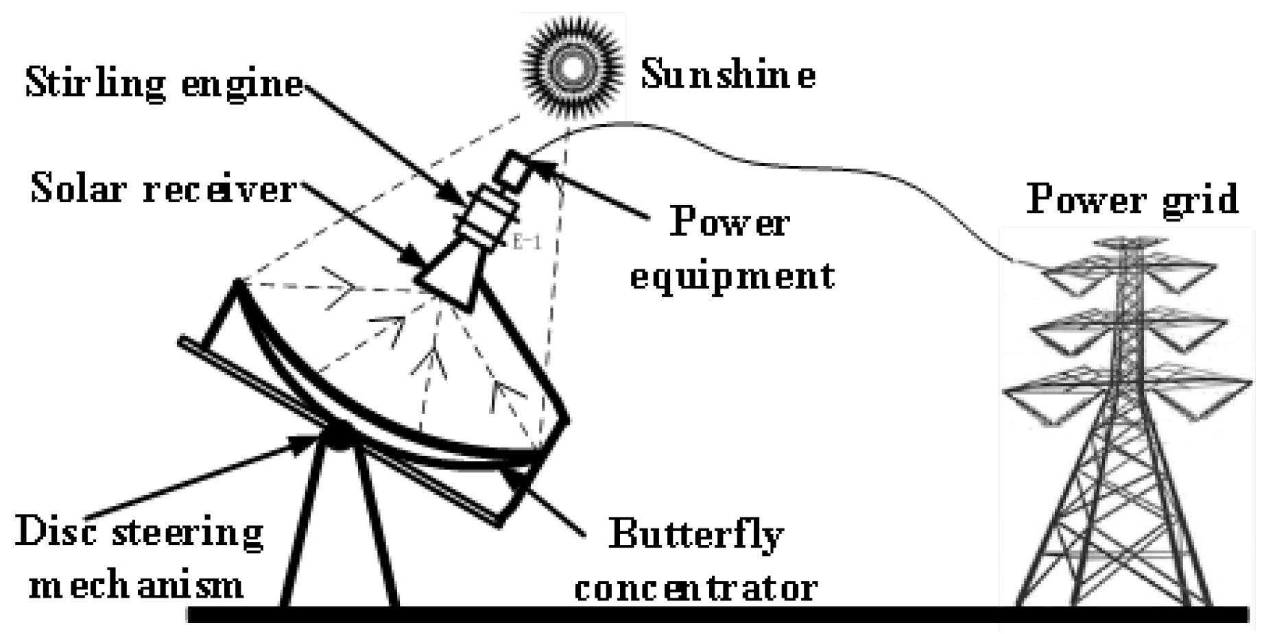
2.1. Mathematical Model of Solar Stirling Power Generation System

The dish solar Stirling power generation system mainly consists of a solar concentrator, a solar absorber, a Stirling heat engine, and a Stirling heat engine driven generator as shown in Figure 1. A dish concentrator is usually a mirrored device made of highly reflective material for reflecting sunlight. The reflected sunlight converges to the focal point of the paraboloid, and the heat sink placed at the focus absorbs the concentrated solar energy into the cavity. The internal cavity of the heat sink is equipped with a heat pipe filled with a working medium, and the working medium converts the absorbed solar energy into heat energy and transmits the heat to the Stirling generator to provide a heat source for the Stirling generator. The mechanical energy output from the generator can be converted into electrical energy by connecting a DC generator to the end of the Stirling generator. Interested readers may refer to [34] for more detailed description and model derivations for solar-dish Stirling system.

The solar Stirling power generation system model has three objective functions to optimize, namely, the maximizing output power, maximizing thermal efficiency, and minimizing entropy yield [35]. It should be noted that these three objective functions are contradictory. For example, increasing the output power will result in a decrease in thermal efficiency.

2.1.1. Decision Variables

The solar Stirling power generation system has seven design parameters to be optimized including the efficiency of the high temperature heat exchanger, the efficiency of the low temperature heat exchanger, the efficiency of the heat sink, the efficiency of the heat source, the temperature of the working medium in the high temperature isothermal process and the temperature of the working medium in the low temperature isothermal process. These variables and their range of values are shown in the

Table 1. Design parameters and range of values for solar Stirling generator systems [34].

Variable Name	Symbol	Minimum Value	Maximum Value
Effectiveness’s of regenerator	${\epsilon }_R$	0.4	0.8
Effectiveness’s of the low temperature heat exchanger	${\epsilon }_H$	0.4	0.9
Effectiveness’s of thehigh temperature heat exchanger	${\epsilon }_L$	0.4	0.9
Heat capacitance rate of the heat sink	$C_H\left(\mathrm{W}{\mathrm{K}}^{-1}\right)$	300	1800
Heat capacitance rate of the heat source	$C_L\left(\mathrm{W}{\mathrm{K}}^{-1}\right)$	300	1800
Working temperature in high temperature isothermal process	$T_h\left(\mathrm{K}\right)$	800	1000
Working temperature in low temperature isothermal process	$T_c\left(\mathrm{K}\right)$	400	510

.

2.1.2. Constants

In addition to the seven design variables, the solar Stirling power generation system model has several constants. Their values are shown in

Table 2. Constant parameters of solar Stirling generator system [34].

Parameter	Value	Parameter	Value	Parameter	Value
$I\left(\mathrm{W}{\mathrm{m}}^{-2}\right)$	1000	$h\left(\mathrm{W}{\mathrm{m}}^{-2}{\mathrm{K}}^{-1}\right)$	20	$T_{L1}\left(\mathrm{K}\right)$	290
$C_{\nu }\left(\mathrm{Jmo}{\mathrm{l}}^{-1}{K}^{-1}\right)$	15	$\epsilon$	0.9	$1/M1+1/M2\left(\mathrm{s}{\mathrm{K}}^{-1}\right)$	$2\times {10}^{-5}$
$\xi$	$2\times {10}^{-10}$	$T_{H1}$	1300	n	1
$C\left(\mathrm{W}{\mathrm{K}}^{-1}\right)$	1300	$\lambda$	2	$T_0\left(\mathrm{K}\right)$	288
$R\left(\mathrm{Jmo}{\mathrm{l}}^{-1}{\mathrm{K}}^{-1}\right)$	4.3	$K_0\left(\mathrm{W}/\mathrm{K}\right)$	2.5	$\delta \left(\mathrm{W}{\mathrm{m}}^{-2}{\mathrm{K}}^{-4}\right)$	$5.67\times {10}^{-8}$

.

2.1.3. Objective Function

The parameter used in calculating the objective function of the Stirling model are shown in

Table 3. Parameter used in the objective function for the Stirling model.

Parameter	Explanation
$P_S$	maximize output power of the Stirling model
$Q_H$	the net heat released from the heat source
$Q_L$	the net heat absorbed by the radiator
$t_{cycle}$	the cycle period of the system
$Q_h$	the heat released from the heat source to the working fluid
$Q_c$	the heat absorbed by the cooling radiator from the working fluid
$Q_0$	the heat transfer loss from the heat source to the heat sink
${\eta }_m$	the overall efficiency of the system
${\eta }_s$	the product of the collector efficiency
${\eta }_t$	the Stirling engine efficiency
$\sigma$	minimize entropy production rate
$T_{Lave}$	the average temperature of heat source
$T_{Have}$	the average temperature of heat sink

.

(1) Maximize output power

$$Max{f}_1=P_S=\frac{Work}{Time}=\frac{Q_H-Q_L}{t_{cycle}}$$

(1)

where $Q_H$ and $Q_L$ are the net heat released from the heat source and absorbed by the radiator, respectively, $t_{cycle}$ is the cycle period of the system [34], the specific calculation formula is given as follows [35]:

$$Q_H=Q_h+Q_0$$

(2)

$$Q_L=Q_c+Q_0$$

(3)

$$t_{cycle}=\frac{nR{T}_{h}ln\lambda +n{C}_{\nu }(1-{\epsilon }_R)(T_h-T_c)}{C_H{\epsilon }_H(T_{H1}-T_h)+\xi C_H{\epsilon }_H(T_{H1}^4-T_h^4)}+\frac{nR{T}_{h}ln\lambda +n{C}_{\nu }(1-{\epsilon }_R)(T_h-T_c)}{C_L{\epsilon }_L(T_c-T_{L1})}+(\frac{1}{M1}+\frac{1}{M2})(T_h-T_c)$$

(4)

where $Q_h$, $Q_c$, $Q_0$ are the heat released from the heat source to the working fluid, the heat absorbed by the cooling radiator from the working fluid, and the heat transfer loss from the heat source to the heat sink, respectively, and M1 and M2 are the regeneration constants in heating and cooling engineering. The specific expression is given as follows:

$$Q_h=nR{T}_{h}ln\left(\lambda \right)+n{C}_{\nu }(1-{\epsilon }_R)(T_h-T_c)$$

(5)

$$Q_c=nR{T}_{c}ln\left(\lambda \right)+n{C}_{\nu }(1-{\epsilon }_R)(T_h-T_c)$$

(6)

$$Q_0=\frac{K_0}{2}[(2-{\epsilon }_H)T_{H1}-(2-{\epsilon }_L)T_{L1}+({\epsilon }_H{T}_h-{\epsilon }_L{T}_c)]t_{cycle}$$

(7)

where n is the molar constant, R is the gas constant, $\lambda$ is the volume ratio during regeneration, $C_{\nu }$ is the specific heat capacity, ${\epsilon }_R$ is the efficiency of the accumulator, $T_h$ and $T_c$ are the temperatures of working fluid in isothermal process at high temperature and low temperature.

(2) Maximize thermal efficiency

$$Max{f}_2={\eta }_m={\eta }_s{\eta }_t$$

(8)

It can be seen from the expression that the overall efficiency of the system ${\eta }_m$ is the product of the collector efficiency ${\eta }_s$ and the Stirling engine efficiency ${\eta }_t$. The efficiency of the collector and the Stirling engine are as follows:

$${\eta }_s={\eta }_0-\frac{1}{IC}[h(T_{H_{ave}}-T_0)+\epsilon {\sigma }_0(T_{H_{ave}}^4-T_0^4)]$$

(9)

$${\eta }_t=\frac{nR(T_h-T_c)ln\lambda }{nR{T}_{h}ln\lambda +n{C}_{\nu }(1-{\epsilon }_R)(T_h-T_c)+\frac{K_0}{2}[(2-{\epsilon }_H)T_{H_1}-(2-{\epsilon }_L)T_{L_1}+({\epsilon }_H{T}_h-{\epsilon }_L{T}_c)]t_{cycle}}$$

(10)

where ${\eta }_0$ is the optical efficiency of the concentrator, I is the solar incident intensity, C is the heat capacity rate, $\epsilon$ is the emissivity factor of the emitter, ${\sigma }_0$ is the Boltzmann constant, $K_0$ is the coefficient of the heat leakage.

(3) Minimize entropy production rate

$$Max{f}_3=\sigma =\frac{1}{t_{cycle}}(\frac{Q_L}{T_{Lave}}-\frac{Q_H}{T_{Have}})$$

(11)

where $T_{Lave}$ and $T_{Have}$ are the average temperature of heat source and heat sink, the specific calculation formula is as follows:

$$T_{Have}=\frac{T_{H1}+T_{H2}}{2},T_{H2}=(1-{\epsilon }_H)T_{H1}+{\epsilon }_H{T}_h$$

(12)

$$T_{Lave}=\frac{T_{L1}+T_{L2}}{2},T_{L2}=(1-{\epsilon }_L)T_{L1}+{\epsilon }_L{T}_c$$

(13)

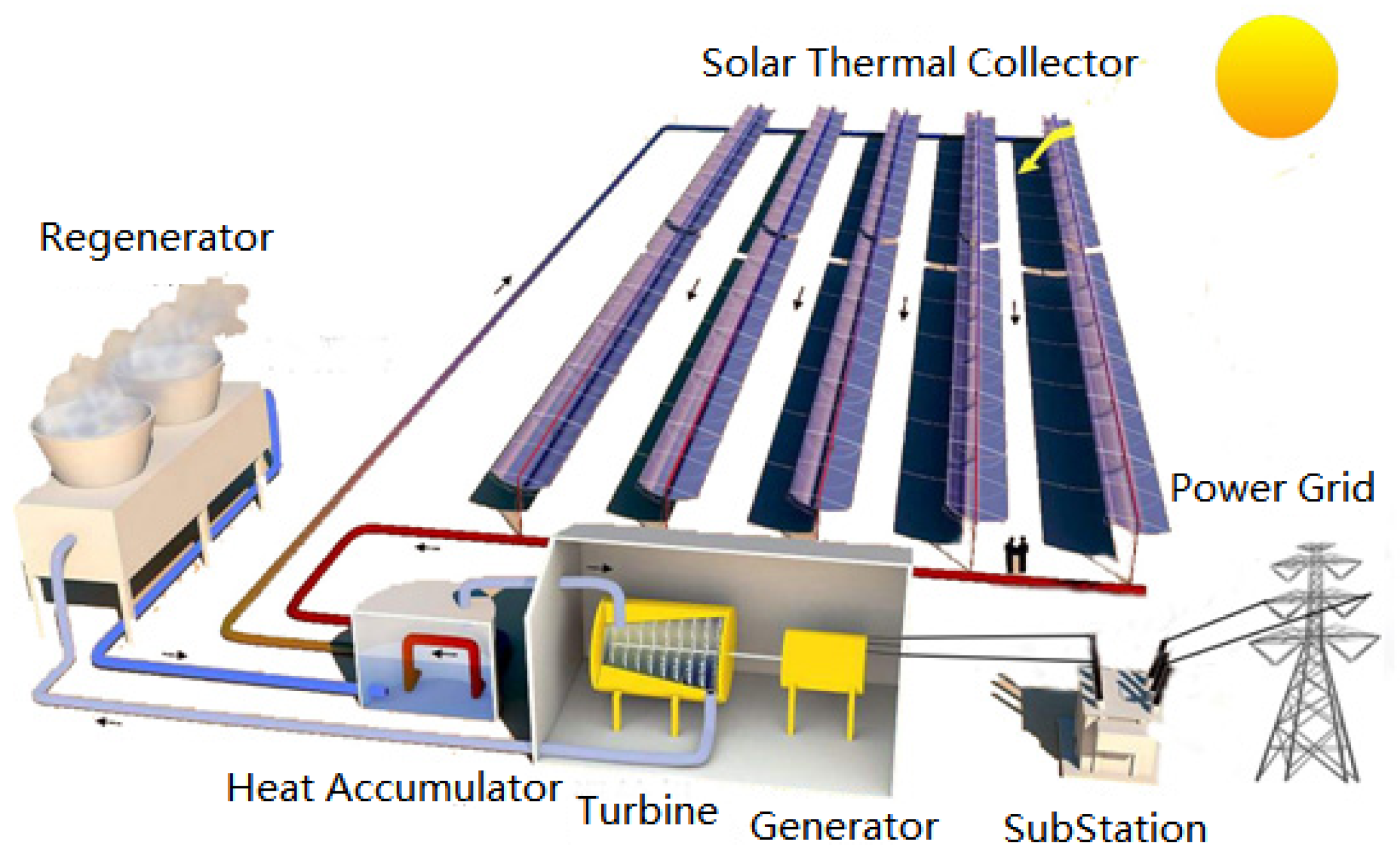
2.2. Mathematical Model of Solar Brayton Power Generation System

The solar Brayton cycle heat engine power generation system has the advantages of high thermal efficiency, light weight, long life and simple structure, so it is widely used in space power stations. Similar to the solar Stirling cycle heat engine power generation system, the solar Brayton heat engine power generation system is mainly composed of a solar-dish concentrator, a heat accumulator, an energy conversion device and a regenerator. Its working disgram is shown in Figure 2. The solar concentrator concentrates the incident solar radiation into a heat accumulator consisting of a plurality of heat exchange tubes arranged in parallel. The circulating fluid is transferred from these heat exchangers. The envelope outside the heat exchange tube contains a certain amount of heat storage material for storing and releasing heat energy, thereby maintaining the temperature of the accumulator outlet working medium fluctuating within a certain range. In the Brayton heat engine cycle, after the compressor pressurizes the gaseous working medium, the high-pressure working medium flows into the regenerator to exchange heat with the working fluid discharged from the turbine, and the heated working medium enters the regenerator and is heated to increase the gaseous working medium temperature and thus the internal energy increases, and then the high-temperature and high-pressure working fluid flows back into the turbine and expands to do work, driving the turbine to generate mechanical energy. This part of the mechanical energy can be used to drive the compressor to compress working medium, and the other part is used to drive the generator to produce electrical energy. Interesting readers may refer to [34] for more detailed description and model derivations for solar-dish Brayton system.

Solar Brayton cycle power generation system optimization is a typical multi-parameter continuous multi-objective optimization problem. In this paper, the model has three optimization objectives, namely maximizing output power, maximizing thermal efficiency and maximizing thermal economic benefits [28]. The relationship between the objective function of the specific optimization model and the optimization parameters is shown in the following section.

2.2.1. Decision Variables and Their Range of Values

In this paper, six optimization parameters are selected as decision variables, and they are listed in

Table 4. Optimized variables and range of values for solar Brayton power generation systems [28].

Variable Name	Symbol	Minimum Value	Maximum Value
High temperature heat exchanger efficiency	${\epsilon }_H$	0.5	0.7
Low temperature heat exchanger efficiency	${\epsilon }_L$	0.5	0.7
Accumulator efficiency	${\epsilon }_R$	0.5	0.8
Heat accumulator high temperature	$T_H\left(K\right)$	700	1000
Heat accumulator low temperature	$T_L\left(K\right)$	400	500
The temperature of the working fluid in the Brayton cycle 1	$T_1\left(K\right)$	$T_L$	$T_H$

:

2.2.2. Constants

In addition to the six optimization variables, the solar Brayton power generation system model has some constants. In order to keep consistent with the previous work, the various constants involved in the model and their respective values are given in

Table 5. Constant parameters of solar Brayton power generation system [28].

Parameter	Value	Parameter	Value	Parameter	Value
${\eta }_0$	0.85	$\delta \left(\mathrm{W}{\mathrm{m}}^{-2}{\mathrm{K}}^{-4}\right)$	$5.76\times {10}^{-8}$	$\xi$	0.02
$I\left(\mathrm{W}{\mathrm{m}}^{-2}\right)$	1000	$h_c\left(\mathrm{W}{\mathrm{m}}^{-2}{\mathrm{K}}^{-1}\right)$	20	$h_H\left(\mathrm{W}{\mathrm{m}}^{-2}{\mathrm{K}}^{-1}\right)$	2000
$R_c$	1300	$T_0\left(\mathrm{K}\right)$	300	$h_L\left(\mathrm{W}{\mathrm{m}}^{-2}{\mathrm{K}}^{-1}\right)$	2000
$e_c$	1300	k	4	${\stackrel{•}{C}}_{wf}\left(\mathrm{W}{\mathrm{K}}^{-1}\right)$	1050

.

2.2.3. Objective Function

The parameter used in calculating the objective function of the Brayton model are shown in

Table 6. Parameter used in the objective function for the Brayton model.

Parameter	Explanation
$P_B$	maximize output power of the Brayton model
${\stackrel{•}{Q}}_{HT}$	the total heat absorption rate in the heat reserve
${\stackrel{•}{Q}}_{LT}$	the total heat release rate released into the cold reserve
${\eta }_m$	maximize thermal efficiency
${\eta }_B$	the Brayton heat engine efficiency
${\eta }_C$	the product of the dish concentrator efficiency
$Q_0$	the heat transfer loss from the heat source to the heat sink
F	maximize thermal economics
$C_i$	annual investment costs
$C_f$	fuel consumption costs
a	minimize entropy production rateXX
b	the annual operating hours per unit of heat input
$A_H$	the hot end of the heat exchange area
$A_L$	the cold end of the heat exchange area

.

(1) Maximize output power

$$P_B={\stackrel{•}{Q}}_{HT}-{\stackrel{•}{Q}}_{LT}$$

(14)

where ${\stackrel{•}{Q}}_{HT}$ and ${\stackrel{•}{Q}}_{LT}$ are the total heat absorption rate in the heat reserve and the total heat release rate released into the cold reserve, respectively, and they are computed using the following formula:

$${\stackrel{•}{Q}}_{HT}={\stackrel{•}{C}}_{wf}{\epsilon }_H[T_H-(1-{\epsilon }_R)T_1-{\epsilon }_R{a}_8]+{\stackrel{•}{C}}_{wf}\xi (T_H-T_L)$$

(15)

$${\stackrel{•}{Q}}_{LT}={\stackrel{•}{C}}_{wf}{\epsilon }_L[(1-{\epsilon }_R)a_8+{\epsilon }_R{T}_1-T_L]+{\stackrel{•}{C}}_{wf}\xi (T_H-T_L)$$

(16)

therefore, the output power can be reformulated as follows:

$$P_B={\stackrel{•}{Q}}_{HT}-{\stackrel{•}{Q}}_{LT}={\stackrel{•}{C}}_{wf}{\epsilon }_H[T_H-(1-{\epsilon }_H)T_1-{\epsilon }_R{a}_8]-{\stackrel{•}{C}}_{wf}{\epsilon }_L[T_H-(1-{\epsilon }_R)a_8+{\epsilon }_R{T}_1-T_L]$$

(17)

(2) Maximize thermal efficiency

$${\eta }_m={\eta }_B{\eta }_C$$

(18)

according to the thermal efficiency expression, the total thermal efficiency of the system is the product of the dish concentrator efficiency ${\eta }_C$ [36,37] and the Brayton heat engine efficiency ${\eta }_B$, which can be expressed as follows:

$${\eta }_B=1-\frac{{\stackrel{•}{Q}}_{LT}}{{\stackrel{•}{Q}}_{HT}}=\frac{{\epsilon }_H[T_H-(1-{\epsilon }_R)T_1-{\epsilon }_R{a}_8]-{\epsilon }_L[(1-{\epsilon }_R)a_8+{\epsilon }_R{T}_1-T_L]}{{\epsilon }_H[T_H-(1-{\epsilon }_R)T_1-{\epsilon }_R{a}_8]+\xi (T_H-T_L)}$$

(19)

$${\eta }_C={\eta }_0-\frac{1}{I{R}_C}[h_c(T_H-T_0)+e_c\delta (T_H^4-T_0^4)]$$

(20)

therefore, the total thermal efficiency of the solar Brayton power generation system is given as follows:

$$\begin{array}{c}{\eta }_m={\eta }_B{\eta }_C=\left\{{\eta }_0-\frac{1}{I{R}_C}[h_c(T_H-T_0)+e_c\delta (T_H^4-T_0^4)]\right\}\times \frac{{\epsilon }_H[T_H-(1-{\epsilon }_H)T_1-{\epsilon }_R{a}_8]-{\epsilon }_L[(1-{\epsilon }_R)a_8+{\epsilon }_R{T}_1-T_L]}{{\epsilon }_H[T_H-(1-{\epsilon }_H)T_1-{\epsilon }_R{a}_8]+\xi (T_H-T_L)}\hfill \end{array}$$

(21)

(3) Maximize thermal economics

$$F=\frac{P}{C_i+C_f}$$

(22)

where $C_i$ and $C_f$ refers to annual investment costs and fuel consumption costs, respectively. The investment cost of a solar Brayton power generation system is assumed to be proportional to the size of the system, which can be proportional to the total heat transfer area. Therefore, the annual investment cost and annual fuel cost of the system can be expressed as follows:

$$\begin{array}{c}{C}_i=a(A_H+A_L)\hfill \\ C_f=b{\stackrel{•}{Q}}_{HT}\hfill \end{array}$$

(23)

where parameter a is equal to the capital recovery factor multiplied by the unit heat transfer area of the investment cost, while b is the annual operating hours per unit of heat input, $A_H$ and $A_L$ are the heat exchange area of hot end and cold end of the heat exchanger, their concrete expressions are as follows:

$$A_H=-\frac{{\stackrel{•}{C}}_{wf}ln(1-{\epsilon }_H)}{h_H}$$

(24)

$$A_L=-\frac{{\stackrel{•}{C}}_{wf}ln(1-{\epsilon }_L)}{h_L}$$

(25)

2.2.4. Restrictions

In this model, the temperature of the Brayton cycle working medium in state 1 must meet certain constraints given below:

$$T_L<T_1<T_H$$

(26)

3. Improved Multi-Objective Particle Swarm Optimization Algorithm

3.1. Traditional Backbone Particle Swarm Optimization Algorithm(BBPSO)

The BBPSO algorithm is an improved particle swarm algorithm proposed by Kennedy [38] in 2003. In the BBPSO algorithm, the speed and update position of the traditional PSO algorithm are replaced with a non-parametric, Gaussian sampling formula based on particle individual leader and global leader:

$$x_{i,j}=N\left(\frac{x{p}_{i,j}+x{g}_j}{2},\left|x{p}_{i,j}-x{g}_j\right|\right)$$

(27)

In addition, an alternative particle update method is also proposed such that each component of the particle has the same probability to select the component corresponding to its individual leader. The update formula is as follows:

$$x_{i,j}=\left\{\begin{array}{cc}N\left(\frac{x{p}_{i,j}+x{g}_j}{2},\left|x{p}_{i,j}-x{g}_j\right|\right)\hfill & ,U(0,1)<0.5\hfill \\ x{p}_{i,j}\hfill & ,else\hfill \end{array}\right.$$

(28)

where $x{p}_{i,j}$ is the jth component corresponding to the individual leader of the i-th particle, $x{g}_j$ is the j-th component corresponding to the global leader, and U(0, 1) is a random number between 0 and 1.

It can be seen that the BBPSO algorithm is compact, simple and does not require any additional control parameters compared with the traditional PSO algorithm.

3.2. Improved Backbone Particle Swarm Optimization Algorithm

The BBMOPSO is a MOPSO algorithm proposed by Zhang [33] in 2012 with relatively fewer control parameters. In the BBMOPSO, the speed and position update operation of the traditional MOPSO are replaced with a non-parametric Gaussian sampling formula. The update not only eliminates the shortcomings of the traditional MOPSO which has dependence on parameter control during particle update, but also improves the optimization performance of the algorithm. The algorithm uses a Gaussian time-varying mutation operation in the mutation phase. According to relevant research, Gaussian mutation has better local search ability, but the ability to guide individuals to jump out of local optimal solution is weak. Therefore the Gaussian mutation operation in the MOPSO may cause the algorithm to converge prematurely, reducing the diversity of the resulting non-inferior solutions.

This paper proposes an improved IBBMOPSO algorthm based on the Cauthy time-varying mutation mechanism based on the above. The mechanism replaces the Gaussian mutation operation of original algorithm with the large-scale Cauthy mutation operator, which increases the global search ability and maintains the diversity of the solutions. Meanwhile an improved cross-border processing mechanism is proposed to further improve the diversity of the traditional cross-border processing mechanism in multi-objective optimization. The IBBMOPSO algorithm is detailed as follows.

(1)

Initialization

The particle swarm with a population size N is initiated, i.e., each particle is assigned with an initial random position within a given range of values. In the initialization phase, the individual leader of each particle is its own, e.g., $x{\overrightarrow{p}}_i={\overrightarrow{x}}_i$, where $x{\overrightarrow{p}}_i$ is the individual leader and ${\overrightarrow{x}}_i$ is the position vector of the i-th particle in particle group $S_0$.

(2)

Update of particle individual leader

The particle individual leader is the best position for the current particle from initialization to the current number of iterations. The IBBMOPSO algorithm uses the following common update method: assuming that the particle position is ${\overrightarrow{x}}_i\left(t\right)$ in the t-th generation, and the individual leader is $x{\overrightarrow{p}}_i\left(t\right)$. If the new particle $x{\overrightarrow{p}}_i(t+1)$ is not dominated by $x{\overrightarrow{p}}_i\left(t\right)$, then $x{\overrightarrow{p}}_i(t+1)$ is ${\overrightarrow{x}}_i\left(t\right)$, otherwise, ${\overrightarrow{x}}_i\left(t\right)$ is still the individual leader of the particle.

In addition, taking the multi-objective function of two targets as an example, the Pareto possession relationship can be described by Figure 3. Among them, the non-inferior solutions of A, B, C, D and E constitute the frontier of Pareto, and they are both Pareto dominant compared to F.

(3)

Selection of Particle global leader

In the single-objective optimization problem, the global leader is generally the best solution currently found by the algorithm. However, for the multi-objective optimization problem, there are conflicts between multiple optimization objectives. It is relatively difficult to determine a single global optimal solution. In IBBMOPSO, the author uses the congestion degree distance measurement technique to select the global leader [39]. Figure 4 takes a two objective optimization problem as an example to give a calculation method for congestion distance measurement:

As shown in the Figure 4, each black dot in the figure represents a solution in the reserve set. The congestion degree of the i-th solution is represented by the average perimeter of the dashed box, and the boundary element of each objective function is regarded as an infinite congestion distance value. Among all particles, the greater the probability that a particle has, a larger congestion value is selected as the global leader.

(4)

Update formula for particle position

The particle update formula of the traditional multi-objective particle swarm optimization algorithm consists of two parts: speed update and position update. In the IBBMOPSO, an improved BBExp method [33] is proposed to update the particle position:

$$x_{i,j}=\left\{\begin{array}{cc}N\left(\frac{rx{p}_{i,j}+(1-r)x{g}_j}{2},\left|x{p}_{i,j}-x{g}_j\right|\right)\hfill & ,U(0,1)<0.5\hfill \\ x{g}_{i,j}\hfill & ,else\hfill \end{array}\right.$$

(29)

In the formula, $x{\overrightarrow{p}}_i$ is the individual leader of the i-th particle, and $x{\overrightarrow{g}}_i$ is the global leader of the i-th particle, where $r\in [0,1]$ in the formula.

(5)

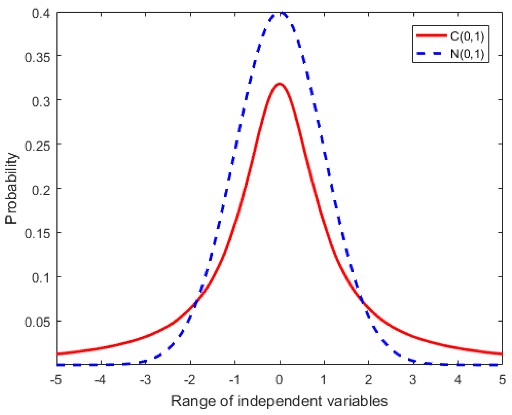
Mutation operator based on Cauchy time-varying mutation mechanism

The role of the mutation operation in the particle swarm optimization algorithm is usually to avoid the algorithm falling into the local optimum. The disturbance operator uses the mutation operator to locate a certain dimensional decision variable of the particle to other search areas, thereby increasing the diversity of the solution. This increases the probability that the algorithm finds the global optimal solution.

In the BBMOPSO, a Gaussian time-varying mutation operator is proposed based on Gaussian variation. The specific mutation operation is shown in Algorithm 1. It can be seen that the operator can adjust the mutation parameter $\alpha$ at the same time. By adjusting the mutation probability and the range of particle activity, as the number of iterations t increases, the mutation probability and activity range of the particle decrease gradually. Therefore, the Gaussian time-varying mutation operator has better local development ability at the later stage of the algorithm iteration.

Algorithm 1: Gaussian time varying mutation operation

1: Function Mutate($\alpha$,t,Bound,$T_{max}$,n) 2: for i=1 to N do 3:     if $p=e^{(-\alpha *t/T_{max})}>r$ then //r:Random number between [0,1] 4:         k=rand(1,n) 5:         range=p*(max_Bound(k)-min_Bound(k)); 6:         $x_{i,k}=x_{i,k}+N(0,1)*range$;//N(0,1):Standard Gaussian distribution function 7:     end if 8: end for

Due to the small variation in Gaussian variation, the ability to guide individuals to jump out of local optimal solutions is weak, so it is not productive to maintaining the diversity of solutions. In this paper, a mutation operator based on Cauchy’s time-varying mutation mechanism is proposed. The specific operation is shown in Algorithm 2. Figure 5 is a comparison of standard Gaussian sampling and Cauchy sampling probability curve. It can be seen that the range of values of the distribution is significantly larger than the Gaussian distribution, so the use of Cauchy time-varying variation is beneficial to increase the diversity of the solution.

Algorithm 2: Cauthy time varying mutation operation

1: Function Mutate($\alpha$,t,Bound,$T_{max}$,n) 2: for i=1 to N do 3:     if $p=e^{(-\alpha *t/T_{max})}>r$ then //r:Random number between [0,1] 4:         k=rand(1,n) 5:         range=p*(max_Bound(k)-min_Bound(k)); 6:         $x_{i,k}=x_{i,k}+C(0,1)*range$; //C(0,1):Standard Cauthy distribution function 7:     end if 8: end for

(6)

Particle out of bounds processing mechanism

When the algorithm performs the update operation and the mutation operation, the limits of variables are often violated. Most algorithms usually adopt the endpoint value method when dealing with such problems, as shown below:

$$x_k=\left\{\begin{array}{c}min\_Bound,\begin{array}{cc}& if\begin{array}{cc}& x_k<min\_Bound\left(k\right)\end{array}\end{array}\\ max\_Bound,\begin{array}{cc}& if\begin{array}{cc}& x_k>max\_Bound\left(k\right)\end{array}\end{array}\end{array}\right.$$

(30)

where $min\_Bound\left(k\right)$ and $max\_Bound\left(k\right)$ are the lower and upper bounds corresponding to the kth dimensional vector, respectively. Different from the single-objective optimization algorithm, since number of objective functions in a multi-objective optimization problem is usually more than two, the optimal solution is no longer unique, but a set of Pareto front-end solution sets. Therefore, in order to increase the diversity of the obtained solutions, the multi-objective algorithm performs a large variation on the solution vector, therefore the chance of limit violations will increase accordingly. The use of conventional endpoint value method for out-of-bounds processing often results in loss of population diversity, especially for optimization problems with more than three goals. In view of the above shortcomings, this paper proposes the following particle out-of-bounds processing:

$$d_k=\beta \times (max\_Bound\left(k\right)-min\_Bound\left(k\right))$$

(31)

$$x_k=\left\{\begin{array}{c}min\_Bound+rand\times d_k,\begin{array}{cc}& if\begin{array}{cc}& x_k<min\_Bound\left(k\right)\end{array}\end{array}\\ max\_Bound-rand\times d_k,\begin{array}{cc}& if\begin{array}{cc}& x_k>max\_Bound\left(k\right)\end{array}\end{array}\end{array}\right.$$

(32)

In the formula, $\beta$ is the endpoint adjustment factor (the particle crossover treatment is better when tested at $\beta$ = 0.01), and rand is a random number between [0, 1]. In the above-mentioned particle out-of-bounds processing mechanism, the out-of-boundary particles randomly generate a value close to the boundary within a certain disturbance range, thus avoiding the loss of population diversity caused by all the out-of-boundary particles taking the endpoint value, thereby increasing the diversity of the population.

(7)

Update of the reserve set

At present, there are many ways to update the external reserve set. This paper uses the method based on the congestion distance measurement method proposed by Raquel and Sierra [40] to update the reserve set in IMBPPOPSO. In the case of external reserves and maintenance and repair, the non-inferior solutions in the reserve set are first merged with the non-inferior solutions currently found by the algorithm. If the number of the centralized solution is greater than its fixed capacity $N_a$ at this time, the congestion degree of each solution is calculated, and the first $N_a$ solutions with larger congestion degree are saved to the reserve set according to the congestion degree.

4. Simulation Experiment Analysis

4.1. Multi-Objective Test Environment

4.1.1. Multi-Objective Test Function

In order to evaluate the performance of the improved algorithm, fifteen representative test functions are selected from four multi-objective test function series and optimized, they are DEB, FON, ZDT (1,2,3,4,6) [41].

4.1.2. Multi-Objective Evaluation Index

In the literature, a set of evaluation indicators for multi-objective algorithm performance have been proposed, these methods can be attributed to two categories: the first is used to evaluate the proximity of the search solution to the real Pareto front-end solution which is mainly used to evaluate the convergence of the algorithm; the other is to evaluate the distribution of the obtained solution. In order to evaluate the performance of the multi-objective particle swarm optimization algorithm on the test function, this paper introduces two classic performance evaluation indicators. The specific data evaluation indicators are listed below.

(1)

Inverted General Distance (IGD)

The IGD [42] is used to evaluate the Euclidean distance of the nearest Pareto optimal solution to the nearest Pareto optimal solution set. The formula is as follows:

$$IGD=\frac{\sqrt{{\displaystyle \sum _{i=1}^{\left|Q\right|}}{d}_i^2}}{\left|Q\right|}$$

(33)

$$d_i=min\left\{\sqrt{\sum {(f_j^{\left(i\right)}-f_j^{*\left(k\right)})}^2}\right\},k=1,2,\dots ,\left|Q^{*}\right|$$

(34)

where Q represents the Pareto optimal solution set found by the multi-objective algorithm, $\left|Q\right|$ represents the number of non-inferior solutions in Q, $Q^{*}$ represents the theoretical Pareto optimal solution set, $\left|Q^{*}\right|$ represents the number of non-inferior solutions, and $d_i$ represents the distance from the first non-inferior solution found to the theoretically closest Pareto optimal solution, and $f_j^{\left(i\right)}$ is the j-th objective function value of the i-th solution in Q, $f_j^{*\left(k\right)}$ is the j-th objective function value of the k-th solution. If IGD=0, it means that all solutions found are in the Pareto optimal solution set, so the smaller the IGD the better performance.

(2)

Hyper Volume (HV)

The HV [43] is used to calculate the super-volume of the coverage area determined according to the position of all the points in the obtained non-dominated solution set. The index can comprehensively determine the convergence and diversity, which are defined as follows:

$$I_H=volume\left({\displaystyle \underset{i=1}{\overset{\left|F\right|}{\cup }}}{\nu }_i\right)$$

(35)

All the values usually need to be normalized before calculating the super volume index. When the calculation is completed, the obtained solution can be analyzed according to the size of the super volume index. The larger the value of the super volume, the closer the resulting non-inferior solution front is to the true Pareto optimal solution, and the better the distribution of the solution. Therefore, the convergence of the Pareto solution relative to the true Pareto optimal solution frontier and the distribution diversity of each point in the solution set can be comprehensively measured by this index.

(3)

Multi-objective comparison algorithm

In this paper, a multi-objective immune algorithm, three multi-objective evolutionary algorithms and two different multi-objective PSO algorithms are compared with the IBBMOPSO. They are NSGA2, SPEA2, PAES2, MOPSO and BBMOPSO algorithm. The population size and the reserve size of all the algorithms are set as the 100.

Table 7. Parameter setting of the algorithm.

Algorithm	Parameter
NSGA2	The variation coefficient of variation is set to 20
	The probability of variation is 3
	The probability of crossover is 0.9
	Bidding selection
SPEA2	The exchange probability is set to 0.5
	The two mutation probabilities are 0.2
	The two crossover probabilities are 0.8
	Bidding selection
PESA2	The number of grids is 7
	The probability of crossover is 0.5
	The probability of mutation is 0.5
MOPSO	The number of grids is 7
	The probability of mutation is 0.1
	Both the individual and the global learning factors are 1 and 2
	The inertia weight is $\omega$ = 0.5
BBMOPSO	Mutation parameter $\alpha$ = 10
IBBMOPSO	Mutation parameter $\alpha$ = 10
	Point adjustment factor $\beta$ = 0.01

shows the other specific parameter settings for the six algorithms including the IBBMOPSO algorithm.

4.2. Simulation Results and Performance Analysis

In order to evaluate the optimization performance of IBBMOPSO algorithm, this paper compares it with three representative multi-objective evolutionary algorithms (NSGA2, SPEA2 [44], PESA2 [45]) and two different multi-objective particle swarm optimization algorithms (MOPSO, BBMOPSO). A multi-target performance index was compared and analyzed. The algorithm performed 30 simulation experiments on 12 test functions. In order to compare the different algorithms, a fair time measure must be selected. The number of iterations cannot be used as a time measure, as the algorithms do differing amounts of work in their inner loops. It was, therefore, decided to use the number of function evaluations (FES) as a time measure [46]. In this paper, the maximum FES (function evolutions) of a test function is set to 15,000 times.

Table 8. Comparison of various evolutionary algorithms IGD indicators.

test function	NAGA2	SPEA2	PESA2	MOPSO	BBMOPSO	IBBMOPSO
DEB	1.7490 × 10${}^{-4}$	1.8600 × 10${}^{-4}$	1.5721×10${}^{-4}$	1.8470 × 10${}^{-4}$	1.5404 × 10 ${}^{-4}$	1.4061 × 10${}^{-4}$
FON	2.4048 × 10${}^{-4}$	1.8560 × 10${}^{-4}$	3.1648 × 10${}^{-4}$	0.0029	1.8636 × 10${}^{-4}$	1.3385 × 10${}^{-4}$
ZDT1	0.0833	8.5192 × 10${}^{-5}$	0.0055	0.0057	8.9124 × 10${}^{-5}$	8.5016 × 10${}^{-5}$
ZDT2	0.2426	9.3335 × 10${}^{-5}$	0.0151	0.1074	1.4219 × 10${}^{-4}$	8.4975 × 10${}^{-5}$
ZDT3	0.0757	1.8114 × 10${}^{-4}$	0.0108	0.0172	1.5631 × 10${}^{-4}$	1.4031 × 10${}^{-4}$
ZDT4	2.7766	0.0953	1.0983	7.5984	2.2880 × 10${}^{-4}$	6.0598 × 10${}^{-5}$
ZDT6	0.1006	2.2246 × 10${}^{-4}$	0.0366	0.1510	7.2898 × 10${}^{-5}$	8.0147 × 10${}^{-5}$

compares the performance of IBBMOPSO algorithm and the IGD index with other algorithms. IGD is used to evaluate the Euclidean distance between the nearest Pareto optimal solution and the theoretical Pareto optimal solution. The smaller the IGD value, the closer the distance of the non-inferior solution to the optimal Pareto front end. It is obvious that IBBMOPSO has better IGD characteristics than other algorithms, in particular, for the functions DEB, FON, ZDT1, ZDT2, ZDT3, ZDT4, it has the best IGD characteristics, and it has the second best IGD for ZDT6. It is clear that the proposed method has overall better IGD index than other algorithms which means that the searched non-inferior dissociation is the closest to the theoretical optimal frontier. Finally, we should note that although the IBBMOPSO algorithm does not have IGD as good as BBMOPSO for ZDT6, it has the most significant improvements for functions ZDT2 and ZDT4. For other functions, a small improvement in IGD is also achieved.

Table 9. Comparison of various evolutionary algorithms HV indicators.

Test Function	NAGA2	SPEA2	PESA2	MOPSO	BBMOPSO	IBBMOPSO
DEB	0.4584	0.4600	0.4647	0.4626	0.4708	0.4721
FON	0.3086	0.2400	0.2490	0.2807	0.3048	0.3102
ZDT1	0.4321	0.6200	0.5740	0.6301	0.6580	0.6595
ZDT2	0.0571	0.3200	0.2480	0.1720	0.3050	0.3261
ZDT3	0.4403	0.7000	0.6840	0.7610	0.7500	0.7612
ZDT4	0.1204	0.5500	0.7700	0.0080	0.0730	0.1228
ZDT6	0.6370	0.2400	0.5220	0.6910	0.2823	0.2840

gives the super-volume index data of IBBMOPSO and other algorithms. It can be seen from the table that SPEA2 has better performance for function ZDT4, PESA2 is better for function ZDT6, while IBBMOPSO is better for all other functions. Therefore, among these algorithms, the IBBMOPSO algorithm is the best to strike the balance between the convergence and diversity.

5. Application of IBBMOPSO to the Optimization of Solar Power Systems

In this paper, we use NSGA2, MOPSO and IBBMOPSO to optimize each model and obtain a series of Pareto solutions. This paper uses three different multi-objective decision-making methods.

5.1. Multi-Objective Optimization Methods

5.1.1. Fuzzy Optimization

The fuzzy optimization [47] represents each objective function value by introducing a linear membership function. The membership function is defined as follows:

$$u_i=\left\{\begin{array}{cc}1& f_i\le f_i^{min}\\ \frac{f_i^{max}-f_i}{f_i^{max}-f_i^{min}}& f_i^{min}\le f_i\le f_i^{max}\\ 0& f_i\ge f_i^{max}\end{array}\right.$$

(36)

Where $f_i^{min}$ and $f_i^{max}$ are the minimum and maximum values of the i-th objective function corresponding to all the program sets, and the membership function value $u_i$ varies between 0 and 1. The larger the value of $u_i$, the better the compatibility of the solution with the optimal solution set.

For each non-dominated solution X, the normalized membership function is defined below:

$$u^k=\frac{{\displaystyle \sum _{i=1}^N}{u}_i^k}{{\displaystyle \sum _{k=1}^M}{\displaystyle \sum _{i=1}^N}{u}_i^k}$$

(37)

where M is the number of scenarios and N is the number of objective functions. $u^k$ can be regarded as a fuzzy combination of the membership function of the non-dominated solution set. In the fuzzy set, the scheme with the highest degree of membership is defined as the best ideal solution.

5.1.2. Linear Programming Method for Multidimensional Analysis of Preference(LINMAP)

The LINMA [48] is a multi-attribute decision-making method based on the ideal solution. It is judged by the decision maker to give a set of ordered scheme pairs that represent the scheme $x_k$ better than the scheme $x_i$ and the index value $a_j^{*}$ of the scheme $x_i$ with respect to the attribute $f_j$, which is established by a linear programming model to find the weight $w_j$ of each attribute and the ideal solution $a_j^{*}$, then use the square of the Euclidean distance

$$S_i={\displaystyle \sum _{j=1}^m}{\omega }_j(a_{ij}-a_j^{*}),i=1,2,\dots ,n$$

(38)

to rank the advantages and disadvantages of the scheme.

5.1.3. Technique for Order Preference by Similarity to an Ideal Solution(TOPSIS)

The TOPSIS method [49] is a method of sorting schemes by means of ideal solutions and negative ideal solutions of multi-objective decision problems. The so-called ideal solution is the best solution. Its various index values can reach the best value of each candidate program, while the negative ideal solution is the worst solution, and its indicators reach the worst value of the solution. Generally speaking, the original solution set usually does not have such ideal solution and negative ideal solution. Therefore, if there is a solution in the solution set that is very close to the ideal solution and away from the negative ideal solution, then the solution can be considered as the best solution in the solution set. Therefore, when the TOPSIS method is used to solve multi-objective decision problems, a measure is defined in the objective space to measure the extent to which a solution is close to the ideal solution and away from the negative ideal solution.

Suppose the decision problem of multi-objective systems with n scenarios and m indicators is studied. The distance $S_i^{*}$ from solution $X^i=(x_{i1},\dots ,x_{im})$ to ideal solution $X^{*}=(x_1^{*},\dots ,x_m^{*})$ and the distance $S_i^{-}$ to $X^{-}=(x_1^{-},\dots ,x_m^{-})$ of the negative ideal solution are:

$$S_i^{*}=\sqrt{{\displaystyle \sum _{j=1}^m}{(X_{ij}-X_j^{*})}^2},i=1,2,\dots n;j=1,2,\dots ,m$$

(39)

$$S_i^{-}=\sqrt{{\displaystyle \sum _{j=1}^m}{(X_{ij}-X_j^{-})}^2},i=1,2,\dots n;j=1,2,\dots ,m$$

(40)

where $X_{i,j}$ is the normalized value of the jth indicator of solution $X^i$: $X_j^{*}$ and $X_j^{-}$ are the jth component of the ideal solution $X^{*}$ and the negative ideal solution $X^{-}$. The relative proximity of the merits and demerits of the solution is $C_i^{*}$:

$$C_i^{*}=S_i^{*}/(S_i^{*}+S_i^{-}),0\le C_i^{*}\le 1,i=1,2,\dots ,n$$

(41)

when $X^i$ is the ideal solution, then $C_i^{*}=1$; when $X^i$ is the negative ideal solution, then $C_i^{*}=0$. Prioritize the schemes in order of $C_i^{*}$ from the largest to the smallest.

5.2. Simulation Experiments

5.2.1. Algorithm Implementation of Multi-objective Engineering Design Problem

In order to optimize, compare and analyze the two power generation system models with the selected three multi-objective algorithms, the specific implementation steps of the algorithm are given below.

Step1: Set the relevant parameters of the algorithm and initialize the population.

Step2: Each algorithm is optimized for each system model and get a series of Pareto solutions.

Step3: For each model, the corresponding optimal solution of each objective function is selected from the Pareto solution set obtained by the three algorithms, and then the optimal solutions obtained by different algorithms for the same target are compared and analyzed.

Step4: Use three different multi-objective decision methods to select the ideal solution from the Pareto solution set obtained by the IBBMOPSO.

5.2.2. Simulation Results for Solar Stirling Power Generation System

This section discusses the optimized mathematical model of the Stirling power generation system. The number of iterations for the three algorithms is set to 10,000.

Table 10. Pareto solution of solar Stirling power generation system.

Stanard	Algorithm	Variable							Objective Function
		${\mathit{\epsilon }}_{\mathit{R}}$	${\mathit{\epsilon }}_{\mathit{H}}$	${\mathit{\epsilon }}_{\mathit{L}}$	${\mathit{C}}_{\mathit{H}}$	${\mathit{C}}_{\mathit{L}}$	${\mathit{T}}_{\mathit{h}}$	${\mathit{T}}_{\mathit{c}}$	${\mathit{P}}_{\mathit{S}}\left(\mathit{kW}\right)$	$\mathit{\sigma }(\mathit{W}/\mathit{K})$	${\mathit{\eta }}_{\mathit{m}}$
Max $P_S$	NSGA-II	0.9	0.6888	0.8	1800	1800	995	503	68,128.6	136.9749	0.29560
	MOPSO	0.9	0.7966	0.8	1800	1800	1000	510	70,286.9	139.2471	0.29554
	IBBMOPSO	0.9	0.8000	0.8	1800	1800	1000	510	70,341.7	139.2852	0.29559
Max $\sigma$	NSGA-II	0.9	0.7582	0.4	1155	300	924	400	9374.07	24.86587	0.30632
	MOPSO	0.9	0.7859	0.7	300	300	989	402	14,021.0	29.39113	0.32472
	IBBMOPSO	0.9	0.4000	0.4	300	300	1000	400	8177.84	21.91929	0.30274
Max $\eta$	NSGA-II	0.9	0.7980	0.8	458	1512	991	400	40,562.1	73.54372	0.34102
	MOPSO	0.9	0.8000	0.8	1800	1800	999	400	61,184.0	106.4823	0.34479
	IBBMOPSO	0.9	0.8000	0.8	1800	1800	1000	400	61,195.2	106.3605	0.34495

shows the NSGA2, MOPSO and IBBMOPSO for the solar Stirling power generation system. Partial Pareto solutions to the objective functions (maximum power output $P_S\left(W\right)$, minimized entropy generation rate $\sigma (W/K)$, maximizing thermal efficiency ${\eta }_m$) are for the individual objectives of the individual targets. The ideal solutions obtained by the three multi-objective decision methods are also given in

Table 11. Pareto solution of solar Stirling power generation system.

Algorithm	Decision Makings	Variable							Objective Function
		${\mathit{\epsilon }}_{\mathit{R}}$	${\mathit{\epsilon }}_{\mathit{H}}$	${\mathit{\epsilon }}_{\mathit{L}}$	${\mathit{C}}_{\mathit{H}}$	${\mathit{C}}_{\mathit{L}}$	${\mathit{T}}_{\mathit{h}}$	${\mathit{T}}_{\mathit{c}}$	${\mathit{P}}_{\mathit{S}}\left(\mathit{W}\right)$	$\mathit{\sigma }(\mathit{W}/\mathit{K})$	${\mathit{\eta }}_{\mathit{m}}$
IBBMOPSO	Fuzzy	0.9	0.8000	0.8	957	1522	1000	400	50,818.9	89.12639	0.34385
	TOPSIS	0.9	0.8000	0.8	984	1291	1000	400	47,353.7	83.33009	0.34338
	LINMAP	0.9	0.8000	0.8	729	1189	1000	400	42,668.9	75.53539	0.34262

.

It can be seen from Table 10 that whether it is for maximizing power output, minimuming the entropy generation rate or maximizing the thermal efficiency, the quality of the best individuals found by IBBMOPSO is higher than the other two algorithms. Figure 6 shows the Pareto optimal frontier distribution of the three algorithms in the optimization design of the solar Stirling power generation system. In addition, the ideal and non-ideal solutions of the model and the ideal solution found by the three multi-objective decision methods are also labelled. It can be seen from the figure that the distribution of solutions searched by the three multi-objective algorithms is roughly the same, but the solution searched by IBBMPSO is superior to NSGA2 and MOPSO both in scope and quality.

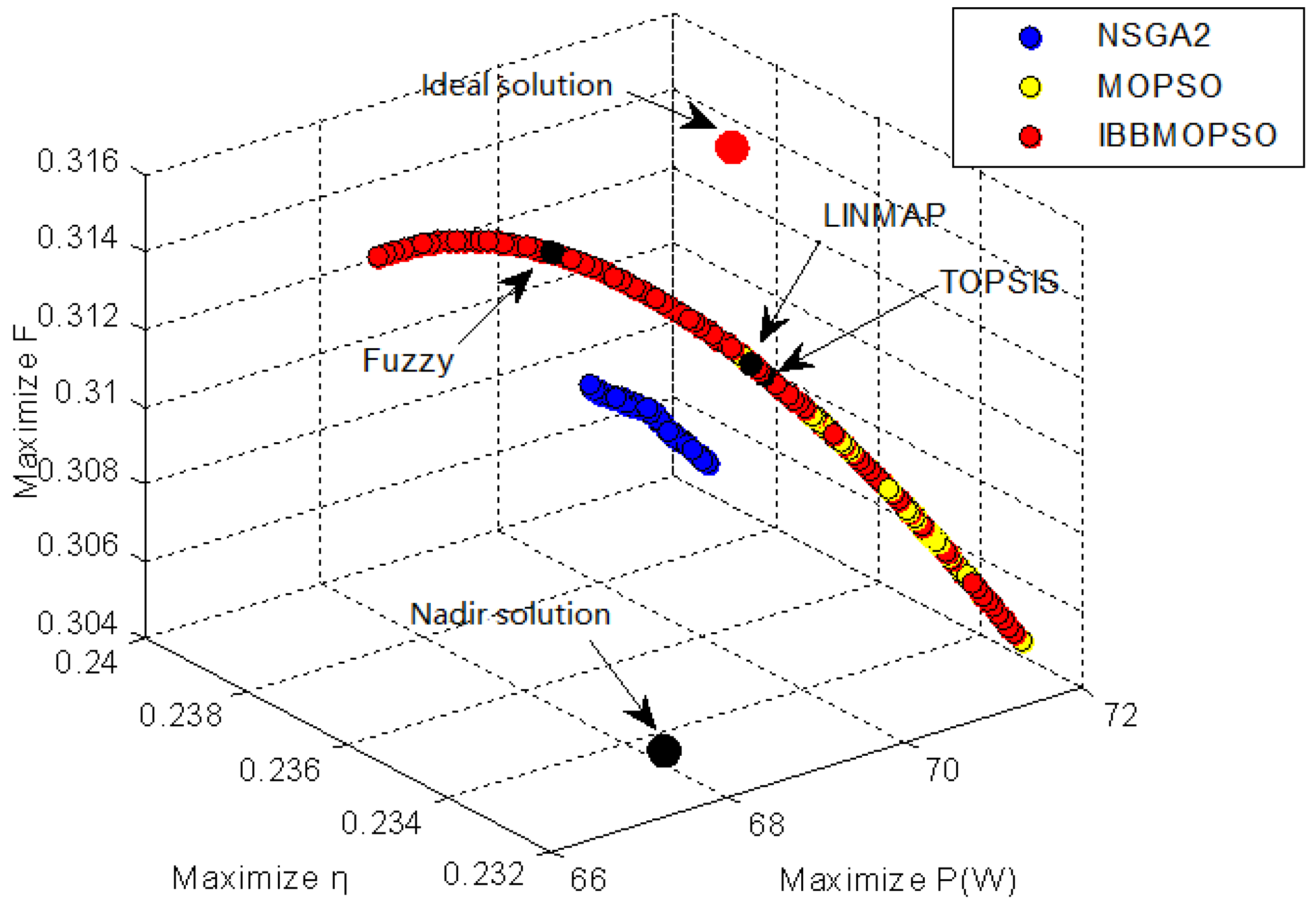
5.2.3. Simulation Results of Solar Brayton Power Generation System

This section presents the results of the optimized mathematical model of the solar Brayton power generation system. The same as the solar Stirling power generation system, the maximum number of iterations of this optimized design is set to 10000 times.

Table 12. Pareto solution of solar Brayton power generation system.

Stanard	Algorithm	Variable						Objective Function
		${\mathit{\epsilon }}_{\mathit{H}}$	${\mathit{\epsilon }}_{\mathit{L}}$	${\mathit{\epsilon }}_{\mathit{R}}$	${\mathit{T}}_{\mathit{H}}$	${\mathit{T}}_{\mathit{L}}$	${\mathit{T}}_1$	${\mathit{P}}_{\mathit{B}}\left(\mathit{kW}\right)$	${\mathit{\eta }}_{\mathit{m}}$	F
	NSGA-II	0.7	0.7	0.8	1000	408	596	68.4118	0.30428	0.23076
	MOPSO	0.7	0.7	0.8	1000	400	600	71.3588	0.30562	0.23206
	IBBMOPSO	0.7	0.7	0.8	1000	400	600	71.3588	0.30562	0.23206
Max $\sigma$	NSGA-II	0.7	0.7	0.8	1000	408	596	68.3864	0.30433	0.23079
	MOPSO	0.7	0.7	0.8	1000	400	567	67.9143	0.31441	0.23776
	IBBMOPSO	0.7	0.7	0.8	1000	400	566	67.8689	0.31443	0.23776
Max $\eta$	NSGA-II	0.7	0.7	0.8	1000	408	596	68.3918	0.30433	0.23079
	MOPSO	0.7	0.7	0.8	1000	400	564	67.3770	0.31450	0.23772
	IBBMOPSO	0.7	0.7	0.8	1000	400	563	67.3226	0.31450	0.23771

shows the single-objective optimal individuals for the optimal power generation $P_B\left(W\right)$, optimal thermal efficiency ${\eta }_m$, and optimal thermal economic efficiency F for the optimal solution of the solar Brayton power generation system. It can be clearly seen from the data marked in the shaded part of the table that the solution found by IBBMOPSO and the MOPSO are the same and superior to NSGA2 in maximizing the power output target. In maximizing thermal efficiency, the best solutions achieved by the IBBMOPSO is superior to the other two algorithms. And the solution produced by the MOPSO that maximizes the thermal economic efficiency is optimal. The ideal solutions obtained by the three multi-objective decision methods are also given in

Table 13. Pareto solution of solar Brayton power generation system.

Algorithm	Decision Makings	Variable						Objective Function
		${\mathit{\epsilon }}_{\mathit{H}}$	${\mathit{\epsilon }}_{\mathit{L}}$	${\mathit{\epsilon }}_{\mathit{R}}$	${\mathit{T}}_{\mathit{H}}$	${\mathit{T}}_{\mathit{L}}$	${\mathit{T}}_1$	${\mathit{P}}_{\mathit{B}}\left(\mathit{W}\right)$	${\mathit{\eta }}_{\mathit{m}}$	F
IBBMOPSO	Fuzzy	0.7	0.7	0.8	1000	400	574	69.1006	0.31360	0.23740
	TOPSIS	0.7	0.7	0.8	1000	400	586	70.4810	0.31074	0.23560
	LINMAP	0.7	0.7	0.8	1000	400	586	70.4194	0.31095	0.23574

.

Figure 7 shows the Pareto frontier distribution optimized by the three multi-objective algorithms for the solar Brayton power generation system. It is obvious that the solution distribution of IBBMOPSO is the widest, and the solution searched by the MOPSO is relatively small. The range only coincides with the solution decomposition searched by the algorithm in this paper, and the solution set searched by the NSGA2 algorithm is not as good as the other two algorithms in terms of the distribution range and the quality of the solution.

6. Conclusions and Future Work

In this paper, an IBBMOPSO algorithm has been proposed based on the BBMOPSO. The experimental results of the improved IBBMOPSO on the test functions show that the IBBMOPSO algorithm has better convergence and distribution than other algorithms. The proposed algorithm is then used to optimize the multi-objective mathematical model of two engineering design problems. The simulation results show that IBBMOPSO has better performance than existing popular approaches. The highlights of this paper cover the following aspects:

• Multi-objective optimization algorithms play an increasingly important role in optimizing the power generation systems from solar energy.
• The IBBMOPSO is proposed based on the BBMOPSO. The experimental results show that IBBMOPSO has better performance than other multi-objective intelligent optimization algorithms.
• IBBMOPSO can provide more options for multi-objective engineering optimization problems than other multi-objective intelligent optimization algorithms.

The proposed IBBMOPSO algorithm has been successfully applied in the optimal design of solar Stirling power generation system and solar Brayton power generation system, and it can be applied to multi-objective engineering optimization design problems.

The MOPSO [6] still has a lot of room for improvement, for example, in developing new particle update strategies and new mutation strategies. The representative external storage file mechanism in the multi-objective optimization can be further improved. Finally, the models of the two generation systems are steady-state models under two assumptions, and the development of more accurate models for the optimal design also deserves future work.

References

1. ExxonMobil. 2018 Outlook for Energy: A View to 2040. Available online: https://corporate.exxonmobil.com (accessed on 25 March 2019).
2. Li, G.Q.; Wang, H.Z.; Zhang, S.L.; Xin, J.T.; Liu, H.C. Recurrent neural networks based photovoltaic power forecasting approach. Energies 2019, 12, 2538. [Google Scholar] [CrossRef]
3. Divina, F.; Torres, M.G.; Vela, F.A.G.; Noguera, J.L.V. A comparative study of time series forecasting methods for short term electric energy consumption prediction in smart buildings. Energies 2019, 12, 1934. [Google Scholar] [CrossRef]
4. UN. United Nations Decade of Sustainable Energy for all 2014–2024. Available online: https://www.un.org/en/sections/observances/international-decades (accessed on 19 July 2018).
5. Vrinceanu, A.; Grigorescu, L.; Dumitrascu, M.; Mocanu, L.; Dumitrica, C.; Micu, D.; Kucsicsa, G.; Mitrica, B.; Vrinceanu. Impacts of photovoltaic farms on the environment in the romanian plain. Energies 2019, 12, 2533. [Google Scholar] [CrossRef]
6. NREL. Assessment of Parabolic trough and Power Tower Solar Technology Cost and Performance Forecast; Report No. NREL/SR-550-34440; NREL: Golden, Co, USA, 2003; pp. 24–28.
7. Leon, L.J. Optimization of Dish Solar Collectors. Energy 1983, 7, 684–694. [Google Scholar]
8. Francisco, N.; Alain, F. Thermal model of a dish Stirling systems. Sol. Energy 2009, 83, 81–89. [Google Scholar]
9. Hafez, A.Z.; Ahmed, S.; Ismail, I.M. Solar parabolic dish Stirling engine system design, simulation and thermal analysis. Energy Convers. Manag. 2016, 15, 60–75. [Google Scholar] [CrossRef]
10. Caballero, G.E.C.; Mendoza, L.S.; Martinez, A.M. Optimization of a dish Stirling system working with DIR-type receiver using multi-objective techiniques. Appl. Energy 2017, 204, 271–286. [Google Scholar] [CrossRef]
11. Li, Y.; Xiong, B.Y.; Su, Y.X.; Tang, J.R.; Leng, Z.W. Particle swarm optimization-based power and temperature control scheme for grid-connected DFIG-based dish-Stirling solar-thermal system. Energies 2019, 12, 1300. [Google Scholar] [CrossRef]
12. Anthony, P. Solar Brayton-cycle power system development. Prog. Aerosp. Sci. 1966, 16, 759–793. [Google Scholar]
13. Springer, T.; Fridfdld, J. Space station freedom solar dynamic power generation. In Technology for Space Station Evolution. Volume 4: Power Systems/Propulsion/Robotics; NASA: Washington DC, USA, 1990; Volume 4, pp. 65–81. [Google Scholar]
14. Meas, M.R.; Bello-Ochende, T. Thermodynamic design optimization of an open air recuperative twin-shaft solar therjal Brayton cycle with combined or exclusive reheating and intercooling. Energy Convers. Manag. 2017, 148, 770–784. [Google Scholar] [CrossRef]
15. Malali, P.D.; Chaturvedi, S.K.; Abdel-Salam, T. Performance optimization of a regenerative Brayton heat engine coupled with a parabolic dish solar collector. Energy Convers. Manag. 2017, 143, 85–95. [Google Scholar] [CrossRef]
16. Khan, M.S.; Abid, M.; Ali, H.M.; Amber, K.P. Comparative performance assessment of solar dish assisted s-CO2 Brayton cycle using nanofluids. Appl. Therm. Eng. 2019, 148, 295–306. [Google Scholar] [CrossRef]
17. Marler, M.T.; Arora, J.S. The weighted method for multi-objetive optimization: New insights. Struct. Multidiscip. Optim. 2010, 41, 853–862. [Google Scholar] [CrossRef]
18. Charnes, A.; Cooper, W.W. Management models and industrial applications of linear programming. Math. Comput. 1962, 16, 401. [Google Scholar] [CrossRef]
19. Ignizio, J.P.; Cavalier, T.M. Linear Programming in Single and Multiple-Objective Systems; Prentice Hall: Upper Saddle River, NJ, USA, 1982. [Google Scholar]
20. Romero, C. Handbook of critical issuues in goal programming. Eur. J. Oper. Res. 1992, 62, 252. [Google Scholar]
21. Yu, P.L. A class of solutions for group decision problems. Manag. Sci. 1973, 19, 936–946. [Google Scholar] [CrossRef]
22. Zeleny, M. Multi-Criteria Decision Making; MCGraw-Hill: New York, NY, USA, 1982. [Google Scholar]
23. Konak, A.; Colt, D.W.; Smith, A.E. Multi-objective optimization using genetic algorithms: A tutorial. Reliab. Eng. Syst. Saf. 2006, 91, 992–1007. [Google Scholar] [CrossRef]
24. Mostaghim, S.; Teich, J. Strategies for finding good local guides in multi-objective particle swarm optimization (MOPSO). In Proceedings of the 2003 IEEE Swarm Intelligence Symposium(SIS 03), Indianapolis, IN, USA, 24–26 April 2003; pp. 26–33. [Google Scholar]
25. Basu, M. Economic environmental dispatch using multi-objective differential evolution. Appl. Soft Comput. 2011, 11, 2845–2853. [Google Scholar] [CrossRef]
26. Zhang, Q.F.; Li, H. MOEA/D: A Multiobjective evolutionary algorithm based on decomposition. IEEE Trans. Evol. Comput. 2007, 11, 712–731. [Google Scholar] [CrossRef]
27. Nazemzadegan, M.R.; Kasaeian, A.; Toghyani, S.; Ahmadi, M.H.; Saidur, R.; Ming, T. Multi-objetive optimization in a finite time thermodynamic method for dish-Stirling by branch and bound method and MOPSO algorithm. Front. Energy 2017, 8, 1701–2095. [Google Scholar]
28. Li, Y.Q.; Liao, S.M.; Liu, G. Thermo-economic multi-objective optimization for a solar-dish Brayton system using NSGA-II and decision making. Int. J. Electr. Power Energy Syst. 2015, 64, 167–175. [Google Scholar] [CrossRef]
29. Li, Y.Q.; Liu, G.; Liu, X.P. Thermodynamic multi-objetive optimization of a solar-dish Brayton system based on the maximum power output, thermal efficiency and ecological performance. Renew. Energy 2016, 95, 465–473. [Google Scholar] [CrossRef]
30. Kennedy, J.; Eberhart, R. Particle swarm optimization. In Proceedings of the International Conference on Neural Networks(ICNN’95), Perth, Australia, 27 November–1 December 1995; pp. 1942–1948. [Google Scholar]
31. Tripathi, P.K.; Bandyopadhyay, S.; Pal, S.K. Adaptive multi-objective particle swarm optimization algorithm. In Proceedings of the IEEE Congress on Evolutionary Compytation, Singapore, 25–28 September 2007. [Google Scholar]
32. Praven, K.T.; Sanghamitra, B.; Sankar, K.P. Multi-Objective Particle Swarm Optimization and Multi-Swarm Concepts and Constraint Handing; Oklahoma State Unversity: Stillwater, OK, USA, 2008. [Google Scholar]
33. Zhang, Y.; Gong, D.W.; Ding, Z.H. A bare-bones multi-objetive particle swarm optimization algorithm for environmental/economic dispatch. Inf. Sci. 2012, 192, 213–227. [Google Scholar] [CrossRef]
34. Ahmadi, M.H.; Mohammadi, A.H.; Dehghani, S.; Barranco-Jimenez, M.A. Multi-objective thermodynamic-based optimization of output power of Solar Dish-Stirling engine by implementing an evolutionary algorithm. Energy Convers. Manag. 2013, 75, 438–445. [Google Scholar] [CrossRef]
35. Punnathanam, V.; Kotecha, P. Multi-objective optimization of Stirling engine systems using Front-based Yin-Yang-Pair Optimization. Energy Convers. Manag. 2017, 133, 332–348. [Google Scholar] [CrossRef]
36. Li, Y.Q.; He, Y.L.; Wang, W.W. Optimization of solar-powered Stirling heat engine with finite-time thermodynamics. Renew. Energy 2011, 36, 421–427. [Google Scholar]
37. Sharma, A.; Shulka, S.K.; Rai, A.K. Finite time thermodynamic analysis and optimization of solar-dish Stirling heat engine with regenerative losses. J. Therm. Sci. 2011, 15, 995–1009. [Google Scholar] [CrossRef]
38. Kennedy, J. Bare bones particle swarms. In Proceedings of the 2003 IEEE Swarm Intelligence Symposium, Indianapolis, IN, USA, 24–26 April 2003. [Google Scholar]
39. Deb, K.; Pratap, A.; Agarwal, S.; Meyarivan, T.A.M.T. A fast and elitist multiobjective genetic algorithm: NSGA-II. IEEE Trans. Evol. Comput. 2002, 6, 182–197. [Google Scholar] [CrossRef]
40. Raquel, C.R.; Naval, P.C. An effective use of crowding distance in multiobjective particle swarm optimization. In Proceedings of the IEEE Congress on Evolutionary Computation, Edinburgh, UK, 2–4 September 2005. [Google Scholar]
41. Zitzler, E.; Deb, K.; Thiele, L. Comparsion of multi-objective evolutionary algorithms: Empirical results. IEEE Trans. Evol. Comput. 2000, 8, 173–195. [Google Scholar]
42. Carlos, A.; Coello, C.; Margarita, R.S. A Study of the parallelization of a coevolutionary multi-objective evolutionary algorithm. In MICAI 2004: Advances in Artificial Intelligence; Springer: Berlin/Heidelberg, Germany, 2004. [Google Scholar]
43. Zitzler, E.; Thiele, L. Multi objective evolutionary algorithms:a comparative case study and the strength Pareto approach. IEEE Trans. Evol. Comput. 1999, 3, 257–271. [Google Scholar] [CrossRef]
44. Lopez-lbanez, M.; Prasad, T.D.; Paechter, B. Multi-objective optimisation of the pump scheduling problem using SPEA2. In Proceedings of the IEEE Congress on Evolutionary Computation, Edinburgh, UK, 2–5 September 2005; pp. 435–442. [Google Scholar]
45. Saha, S.; Bandyopadhyay, S. A generalized automatic clustering algorithm in a multiobjective framework. Appl. Soft Comput. 2013, 13, 89–108. [Google Scholar] [CrossRef]
46. Van den Bergh, F.; Engelbrecht, A.P. A Cooperative Approach to Particle Swarm Optimization. IEEE Trans. Evol. Comput. 2004, 8, 225–239. [Google Scholar] [CrossRef]
47. Wang, H.O.; Tanaka, K.; Griffin, M.F. An approach to fuzzy control of nonlinear systems: Stability and design issues. IEEE Trans. Fuzzy Syst. 1996, 4, 14–23. [Google Scholar] [CrossRef]
48. Srinivasan, V.; Shocker, A.D. Linear programming techniquer for multidimensional analysis of preference. Psychometrica 1973, 38, 337–369. [Google Scholar] [CrossRef]
49. Bellman, R.; Zadeh, L.A. Decision making in a fuzzy environment. Manag. Sci. 1970, 17, 141–164. [Google Scholar] [CrossRef]
Figure 1. Schematic map of the Stirling power system.
Energies 12 04480 g001
Figure 2. Schematic of the Brayton power system.
Energies 12 04480 g002
Figure 3. Schematic diagram of Pareto dominance.
Energies 12 04480 g003
Figure 4. Congestion distance calculation diagram.
Energies 12 04480 g004
Figure 5. Schematic diagram of Pareto dominance.
Energies 12 04480 g005
Figure 6. Pareto frontier map of solar Stirling power generation system.
Energies 12 04480 g006
Figure 7. Pareto frontier map of solar Brayton power generation system.
Energies 12 04480 g007