Research on Multifunctional High-Power Grid Source Simulator System with Synchronous Generator, Line Impedance Imitation, and ZIP Load Emulator

Abstract

As the penetration of distributed power sources in the power grid is getting higher and higher, the adverse effects are also increasing. It is necessary to adopt control technology to make the distributed power source participate in the power regulation of the power system. In this paper, a multifunctional high-power grid source simulator system is presented. For wider control bandwidth and better performance, a high-power, back-to-back converter and an auxiliary lower-power, back-to-back converter connected in cascade mode topology is proposed in this paper. The basic principle and implementation method of virtual synchronous generator (VSG) in the high-power, back-to-back converter are described to reflect the same power frequency characteristics and voltage regulation characteristics as synchronous generators. Amplitude closed-loop control is proposed to realize zero steady-state error in the lower-power, back-to-back converter, also with line impedance imitation. Meanwhile, a constant-impedance, constant-current, and constant-power (ZIP) load model is used to emulate static load in the grid simulator system. At last, a set of experimental results for a 2 MW grid simulator system is provided to verify the effectiveness and validity of the proposed approach.

1. Introduction

With the increasing penetration of distributed generation (DG) [1,2,3,4] and large-scale renewable energy systems, more stringent grid codes [5,6,7,8,9,10,11,12] have been issued to prescribe how those grid-connected systems support the network during grid disturbances. These papers introduce the concept and approach of the European Network Code on Requirements for Generators (NC RfG; EU Commission regulation 2016/631). It provides an overview on the status and details of the implementation in the main national markets for photovoltaic (PV) in Europe. Distributed power generation systems and networks should be carried out before the grid adaptability test. However, the target of the grid is to provide a standard three-phase sinusoidal voltage, thus synchronous generator characteristics are not common. Therefore, during a distributed power generation system test, where it is difficult to recreate the grid conditions through the grid, special equipment to simulate the grid conditions is needed.

To this end, domestic and foreign scholars have done a lot of research. Document [13] proposed the concept of a grid simulator through the d-q coordinate system; the output is no different from the input, but each controller can only track a special frequency harmonic and the algorithm is complex. A 200 kW grid simulator was designed in document [14] to simulate the power grid voltage drop, swells, and high-frequency voltage. A load simulator consisting of resistive, inductive, and capacitive elements was also proposed in this paper, which allowed researchers to simulate a serious work situation of distributed systems, but the circuit composition and control methods of the simulator were not mentioned in this paper, so there were few technical parameters to follow. Three existing grid voltage drop generators were compared in literature [15,16]. Compared with transformer and impedance form, power electronic converter form has stronger functions and wider applicability. Literature [17] researched a kind of multifunctional grid simulator, which can carry on the simulation to the power grid fault conditions, but the harmonic model uses root mean square (RMS) voltage feedback control, and the harmonic frequency cannot be accurately tracked. Literature [18] developed a programmable power grid fault simulation supply, where the inverter part adopts a three-phase bridge-type circuit, making it difficult to simulate grid voltage unbalance. In addition, the double-loop adopts PIR control, which also makes the algorithm become complex.

This paper presents a multifunctional high-power grid simulator system based on a high-power, back-to-back converter and an auxiliary lower-power, back-to-back converter connected in cascade mode topology, with fully accomplished wider control bandwidth and better performance. The fundamental theory and implementation method of the VSG were developed in the high-power, back-to-back converter to embody the same power-frequency characteristics and voltage regulating characteristics as the synchronous generator set. Amplitude closed-loop control was proposed to realize zero steady-state errors in the lower-power, back-to-back converter, also with line impedance imitation. Meanwhile, a constant-impedance, constant-current, and constant-power (ZIP) load model was used to emulate static load in the grid simulator system. A new topology for the high-power grid simulator, together with the corresponding control strategy, enables the grid simulator system to imitate not only the characteristics of a synchronous generator but also harmonic generator characteristics and ZIP load.

The paper is divided into five parts. The first part is the brief introduction of this problem. After that, Section 2 presents a new topology for the high-power grid source simulator system. Section 3 introduces the control strategy of each part in the grid source simulator system. Section 4 describes experimental results and verifies the functionality and performance of the proposed grid source simulator. Finally, Section 5 summarizes the work.

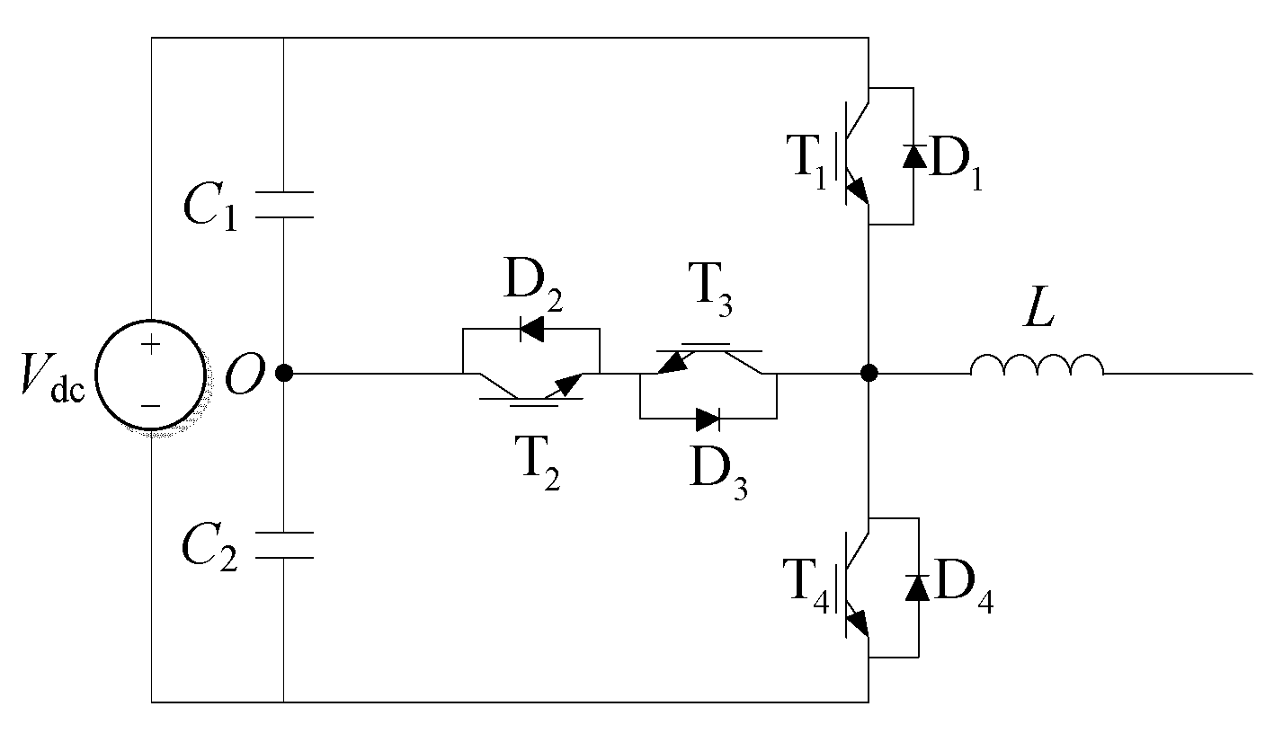
2. A New Topology Design for High-Power Grid Source Simulator

Compared with the low-power grid simulator system, the high-power grid simulator system is much more complex because of its higher power rating, lower switching frequency, and lower control bandwidth, thus reducing the performance of the high-power grid simulator.

Figure 1a shows the picture of the grid simulator system schematics. It includes four parts: the voltage source E_g of the system equivalent generator, the harmonic voltage source E_h of the system harmonic generator, the virtual line impedance Z_s, and the system ZIP load Z_load.

The corresponding grid source simulator system topology is shown in Figure 1b. From the topology, we can see that the voltage source E_g is generated by a high-power, back-to-back, two-level circuit with a fundamental LC filter; the harmonic voltage source E_h is generated by a series of low-power but high switching frequency, back-to-back, three-level circuits with a harmonic LC filter; and the output capacitance voltage of the fundamental LC filter is connected to the output capacitance voltage of the harmonic LC filter through a series injection transformer. The series injection transformer consists of three single-phase injection transformers; each single-phase injection transformer has a double-winding structure, and the three-phase neutral points are connected together. The voltage source E_g series coupling with the harmonic voltage source E_h component is the system source. The virtual line impedance Z_s is realized by the control strategy in the following section. The system ZIP load Z_load is realized by a back-to-back, two-level circuit shown in the topology. The back-to-back topology can realize the four-quadrant operation of energy, and also the feedback energy to the power grid.

The advantage of this new topology is that the voltage source E_g guarantees the power rating of the grid simulator system by using a high-power, back-to-back, two-level circuit while the harmonic voltage source E_h improves the performance of the high-power circuit by increasing the control bandwidth.

3. Control Strategy of Each Part in Grid Source Simulator System

This section may be divided by subheadings. It should provide a concise and precise description of the experimental results, their interpretation, and the experimental conclusions that can be drawn.

3.1. Control Strategy of the Voltage Source E_g: Fundamental Theory and Implementation Method of VSG

The proposed VSG frequency control is analogous to that of a synchronous generator (SG) in Figure 2. Thus, we assume a virtual inertia constant J for the VSG unit, such that speed ω of the voltage space vector of the VSG terminal is governed by the amplitude closed-loop control method of lower-power, back-to-back converter.

$$P_m-P_e=J\omega \frac{d\omega }{dt}\approx J{\omega }_0\frac{d({\omega }_0+\Delta \omega )}{dt}$$

(1)

$$P_m=P_{ref}+\frac{1}{m}({\omega }_0-\omega )$$

(2)

where ω₀ and ω are reference and actual measured values of the converter output angular frequency, respectively, Δω is the difference between ω₀ and ω, P_e is the VSG real output active power, and P_m is the VSG input power defined by the droop characteristic. P_ref is the reference value of the converter output power, m is the active droop constant. The relationship between the VSG terminal voltage angular frequency ω and position θ is

$$\frac{d\theta }{dt}=\omega$$

(3)

where angle θ is given to the VSG controller as a phase command of the VSG output voltage. The frequency control approach, based on (1)–(3), is represented by the block diagram of Figure 2. The proposed voltage controller for the VSG unit is also shown in Figure 2. The VSG terminal voltage U is determined by the voltage droop block.

$$U=U_{\mathrm{o}}+n(Q_{\mathrm{ref}}-Q)$$

(4)

where U_o and Q_ref are the reference values of the converter output voltage and power, respectively. Q is the VSG real output reactive power, n is the reactive droop constant. Apply (2) to (1), so that the reference angular frequency of the VSG can be obtained:

$$\omega ={\omega }_{\mathrm{o}}+\frac{m(P_{ref}-P_e)}{mJ{\omega }_{\mathrm{o}}s+1}$$

(5)

Equation (5) reveals the relation between parameters both from swing Equation (1) and from governor Equation (2). Let J = 0, then (5) is similar to (2). That is to say, droop control can be considered as a particular case of VSG control, where inertia J is equal to zero.

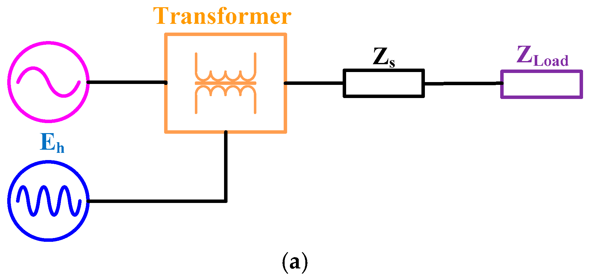
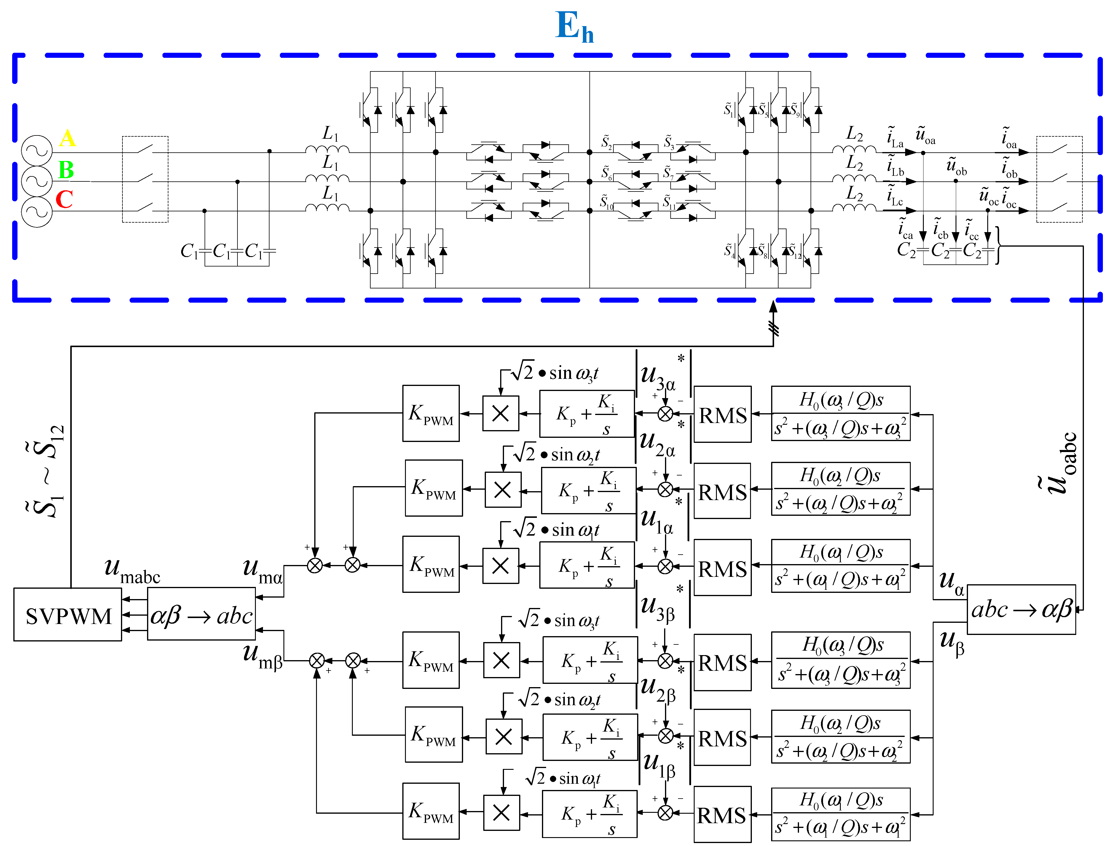
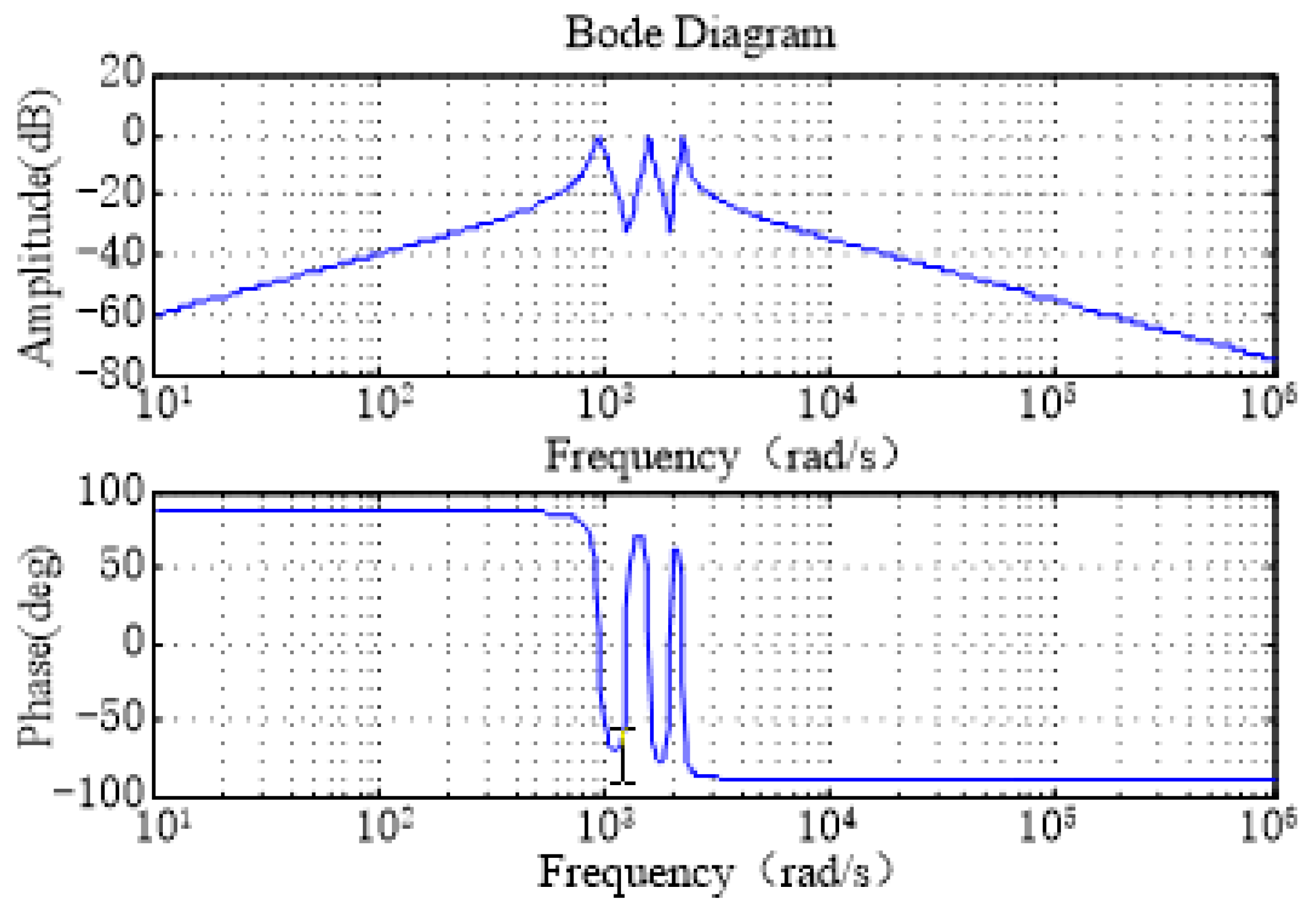
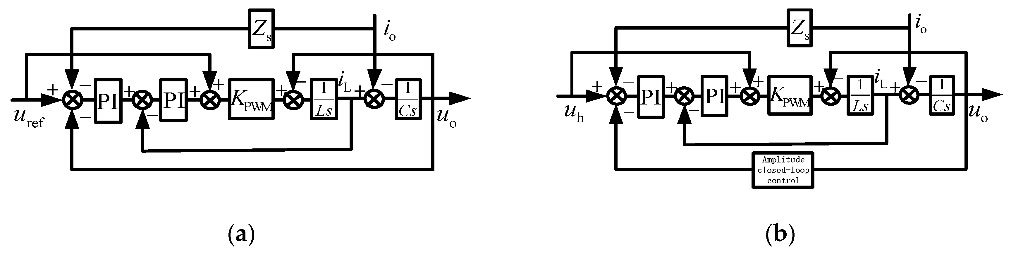
3.2. Control Strategy of the Harmonic Voltage Source E_h

The proposed amplitude closed-loop control is mainly achieved by a band-pass filter and PI controller. Figure 3 shows three harmonic combinations of amplitude closed-loop control. Coordinate transformation simplifies three phases into two phases, separating and extracting harmonics of corresponding frequency segments by using a band-pass filter control, since the amplitude is a scalar so that a PI controller can easily realize zero steady-state error. For example, the transfer function of the control strategy shown in Figure 3 is:

$$H(s)=\frac{H_0({\omega }_1/Q)s}{s^2+({\omega }_1/Q)s+{\omega }_1{}^2}+\frac{H_0({\omega }_2/Q)s}{s^2+({\omega }_2/Q)s+{\omega }_2{}^2}+\frac{H_0({\omega }_3/Q)s}{s^2+({\omega }_3/Q)s+{\omega }_3{}^2}$$

(6)

where ω_n (n = 1,2,3) is central angular frequency; H₀ is the maximum amplitude at the central angular frequency, and the amplitude decreases by 20 dB/dec distance from the central angular frequency; Q_f is the quality factor, which represents the sharpness of the frequency response curve of the filter, usually with a value of 5–10. Figure 4 shows the transfer function bode diagram of the amplitude closed-loop control with three harmonic combinations, among which Q = 5, H₀ = 1, ω₁ = 2π × 150 rad/s, ω₂ = 2π × 250 rad/s, ω₂ = 2π × 250 rad/s. From Figure 4 we can see the voltage at the three central angular frequencies, which is able to be accurately tracked.

Figure 5 shows the simulation waveforms of three harmonic combinations using closed-loop amplitude control. From the waveforms, it can be seen that the proposed control method can accurately separate the combined harmonics and achieve zero error control of the corresponding harmonic voltage amplitude.

3.3. Control Strategy of the Virtual Line Impedance Z_s Imitation

The actual power grid is not an ideal voltage source; the influence of internal resistance and line impedance [19,20,21] of the power grid should be taken into account. At the same time, due to the different impedance of harmonic lines, the problem of uneven power distribution in photovoltaic grid-connected systems needs to be solved urgently. Based on the simulation of ideal voltage source, the multifunctional power grid simulator system proposed in this paper can also simulate the impedance of fundamental and harmonic lines. The control block diagrams are shown in Figure 6a,b, and the closed-loop transfer functions under two control block diagrams are given by Equations (7) and (8).

$$U_o=\frac{((K_{p1}+\frac{K_{i1}}{s})(K_{p2}+\frac{K_{i2}}{s})+1)K_{pwm}}{(K_{p1}+\frac{K_{i1}}{s})(K_{p2}+\frac{K_{i2}}{s})K_{pwm}Cs+L{C}^2{s}^3+Cs+(K_{p2}+\frac{K_{i2}}{s})K_{pwm}}{U}_{ref}-\frac{((K_{p1}+\frac{K_{i1}}{s})(K_{p2}+\frac{K_{i2}}{s})K_{pwm}{Z}_{l}Cs+LC{s}^2+(K_{p2}+\frac{K_{i2}}{s})Cs)}{(K_{p1}+\frac{K_{i1}}{s})(K_{p2}+\frac{K_{i2}}{s})K_{pwm}Cs+L{C}^2{s}^3+Cs+(K_{p2}+\frac{K_{i2}}{s})K_{pwm}}{i}_o$$

(7)

$$U_o=\frac{((K_{p1}+\frac{K_{i1}}{s})(K_{p2}+\frac{K_{i2}}{s})+1)K_{pwm}Chs}{(K_{p1}+\frac{K_{i1}}{s})(K_{p2}+\frac{K_{i2}}{s})K_{pwm}Chs+L{C}^2{h}^2{s}^3+Chs+(K_{p2}+\frac{K_{i2}}{s})K_{pwm}}{U}_h-\frac{((K_{p1}+\frac{K_{i1}}{s})(K_{p2}+\frac{K_{i2}}{s})K_{pwm}{Z}_{l}Chs+LC{h}^2{s}^2+(K_{p2}+\frac{K_{i2}}{s})Chs)}{(K_{p1}+\frac{K_{i1}}{s})(K_{p2}+\frac{K_{i2}}{s})K_{pwm}Chs+L{C}^2{h}^2{s}^3+Chs+(K_{p2}+\frac{K_{i2}}{s})K_{pwm}}{i}_o$$

(8)

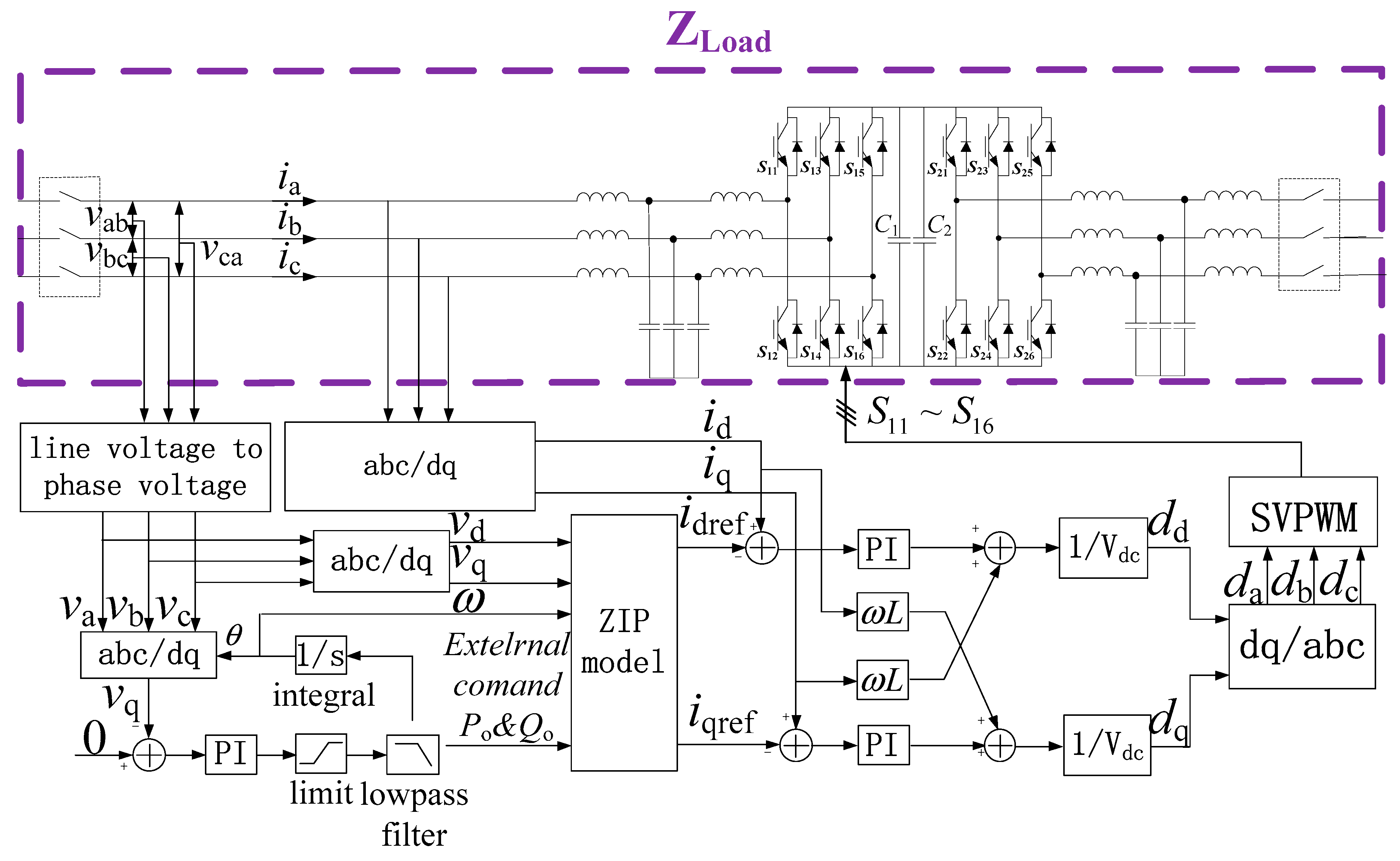
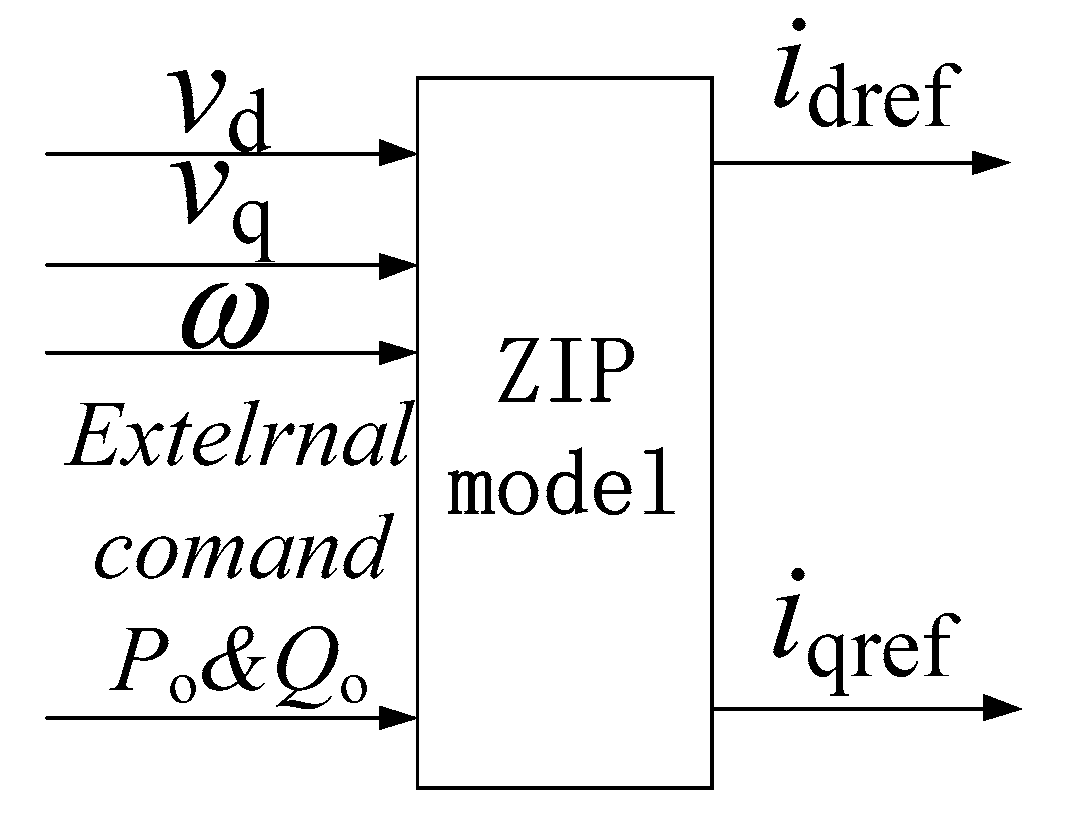
3.4. Control Strategy of the Constant-Impedance, Constant-Current, and Constant-Power (ZIP) Load Z_Load

In power system analysis, the conventional static load model is represented by a series of equations (shown below) which is called ZIP load. They stand for the combination of constant impedance (Z), constant current (I), and constant power (P) loads in both real and reactive power [22,23].

Commonly adopted in power flow calculations, the ZIP model represents the combination of the static characteristics of power system load. Figure 7 shows the control strategy of the ZIP load. The mathematical polynomials are written as (9) and (10) under presumption of minor fluctuation around nominal grid voltage. Also, frequency dependency effect on the load behavior is considered with the coefficients on real and reactive power.

$$P_{\mathrm{ZIP}}=P_{\mathrm{o}}\ast (p_1(\frac{v_{\mathrm{d}}{}^2+v_{\mathrm{q}}{}^2}{V_{\mathrm{o}}{}^2})+p_2(\frac{\sqrt{v_{\mathrm{d}}{}^2+v_{\mathrm{q}}{}^2}}{V_{\mathrm{o}}})+p_3)(1+k_{pf}\Delta f)$$

(9)

$$Q_{\mathrm{ZIP}}=Q_{\mathrm{o}}\ast (q_1(\frac{v_{\mathrm{d}}{}^2+v_{\mathrm{q}}{}^2}{V_{\mathrm{o}}{}^2})+q_2(\frac{\sqrt{v_{\mathrm{d}}{}^2+v_{\mathrm{q}}{}^2}}{V_{\mathrm{o}}})+q_3)(1+k_{\mathrm{qf}}\Delta f)$$

(10)

where P_o and Q_o stand for the real and reactive power reference values, respectively, p₁ and q₁ are coefficients for constant impedance portions for real and reactive power, respectively, while p₂ and q₂ are for constant current portions, p₃ and q₃ are for constant power portions, and k_pf and k_qf are coefficients for the load frequency dependency characteristics.

The ZIP model could be used to fit the power consumption curves for most kinds of power system loads; higher order polynomials are neglected for simplifying the model. In the meantime, the percentage of Z, I, and P for system load could be determined by aggregating different load types and their usage within the grid. By determining the values for p₁, p₂, p₃ and q₁, q₂, q₃, the static load operating state can be specified. It is always set such that the sum of p₁, p₂, p₃ is unity and the sum of q₁, q₂, q₃ is unity.

As presented in Figure 8, the emulated model uses voltages in the dq domain and emulated grid frequency as inputs for the ZIP model. External base real and reactive power commands are given to the model for specifying the actual power desired by customers. Output currents are calculated using the Equations (11) and (12) based on power equivalence relationship in the dq domain. The load emulator current behavior is controlled accurately according to the references so as to ensure the power consumptions at the load bus are the ones described in (13) and (14).

$$i_{\mathrm{dref}}=\frac{v_{\mathrm{q}}{P}_{\mathrm{ZIP}}+v_{\mathrm{d}}{Q}_{\mathrm{Z}\mathrm{I}\mathrm{P}}}{v_{\mathrm{q}}{}^2+v_{\mathrm{d}}{}^2}$$

(11)

$$i_{\mathrm{dref}}=\frac{v_d{P}_{\mathrm{ZIP}}-v_{\mathrm{q}}{Q}_{\mathrm{Z}\mathrm{I}\mathrm{P}}}{v_{\mathrm{q}}{}^2+v_{\mathrm{d}}{}^2}$$

(12)

$$i_{\mathrm{dref}}=\frac{v_{\mathrm{q}}{P}_{\mathrm{o}}(p_1(\frac{v_{\mathrm{q}}{}^2+v_{\mathrm{d}}{}^2}{V_{\mathrm{o}}{}^2})+p_2\frac{\sqrt{v_{\mathrm{q}}{}^2+v_{\mathrm{d}}{}^2}}{V_{\mathrm{o}}}+p_3)(1+k_{\mathrm{pf}}\Delta f)+v_{\mathrm{d}}{Q}_{\mathrm{o}}(q_1(\frac{v_{\mathrm{q}}{}^2+v_{\mathrm{d}}{}^2}{V_{\mathrm{o}}{}^2})+q_2\frac{\sqrt{v_{\mathrm{q}}{}^2+v_{\mathrm{d}}{}^2}}{V_{\mathrm{o}}}+q_3)(1+k_{\mathrm{qf}}\Delta f)}{v_{\mathrm{q}}{}^2+v_{\mathrm{d}}{}^2}$$

(13)

$$i_{\mathrm{qref}}=\frac{v_{\mathrm{d}}{P}_{\mathrm{o}}(p_1(\frac{v_{\mathrm{q}}{}^2+v_{\mathrm{d}}{}^2}{V_{\mathrm{o}}{}^2})+p_2\frac{\sqrt{v_{\mathrm{q}}{}^2+v_{\mathrm{d}}{}^2}}{V_{\mathrm{o}}}+p_3)(1+k_{\mathrm{pf}}\Delta f)-v_{\mathrm{q}}{Q}_{\mathrm{o}}(q_1(\frac{v_{\mathrm{q}}{}^2+v_{\mathrm{d}}{}^2}{V_{\mathrm{o}}{}^2})+q_2\frac{\sqrt{v_{\mathrm{q}}{}^2+v_{\mathrm{d}}{}^2}}{V_{\mathrm{o}}}+q_3)(1+k_{\mathrm{qf}}\Delta f)}{v_{\mathrm{q}}{}^2+v_{\mathrm{d}}{}^2}$$

(14)

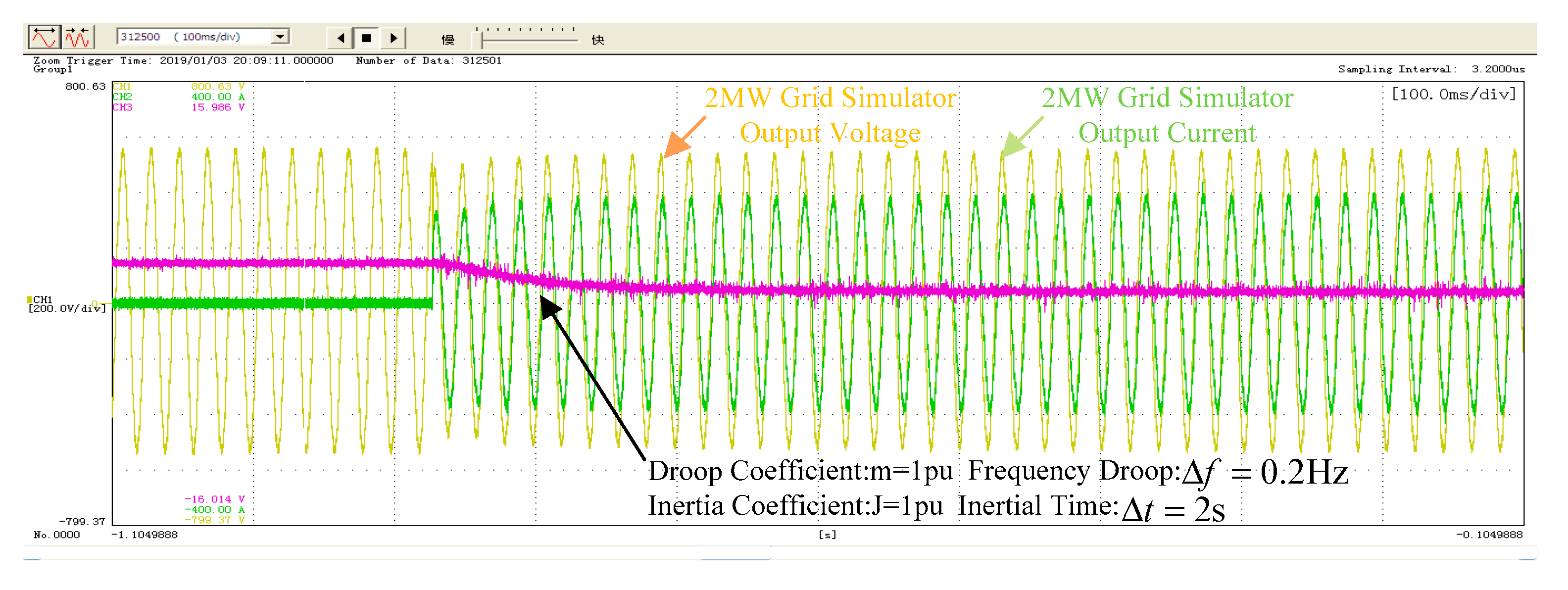
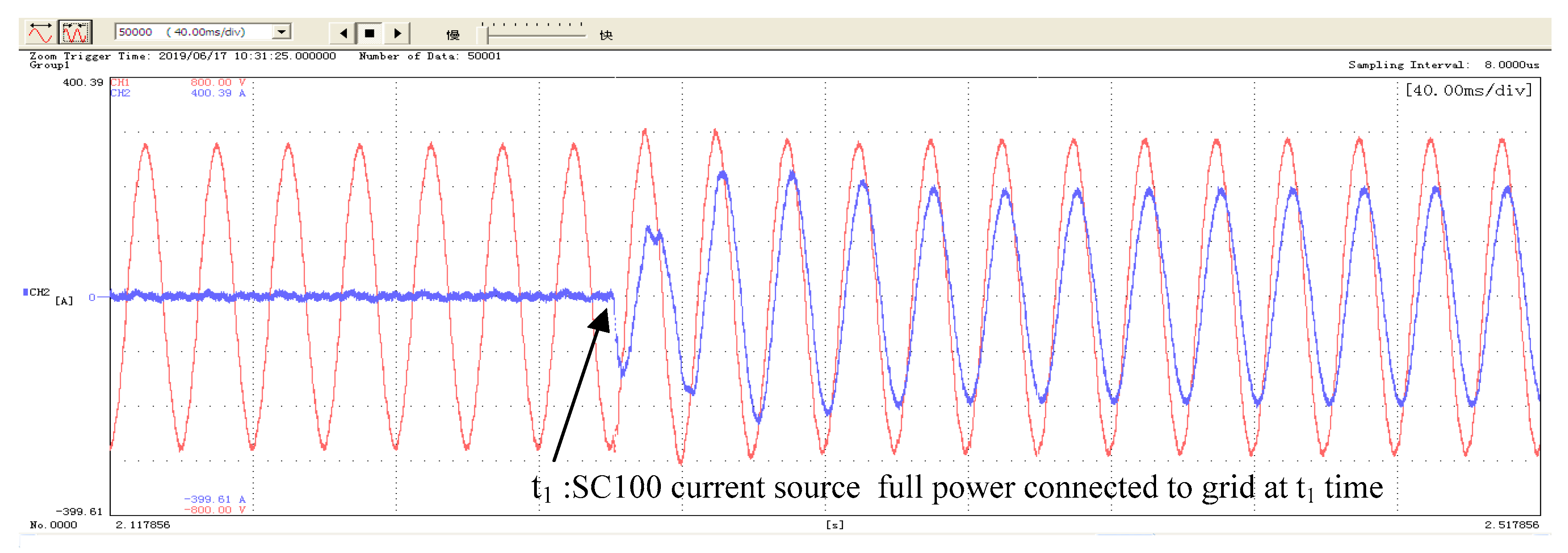
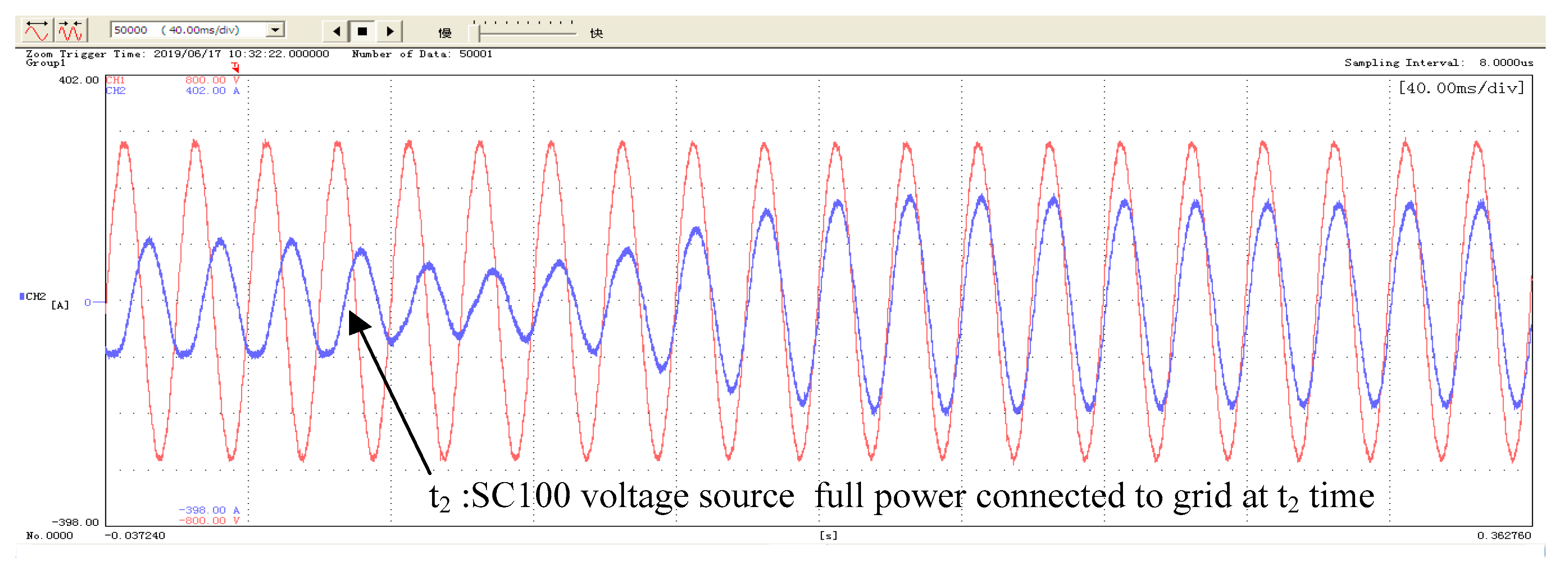
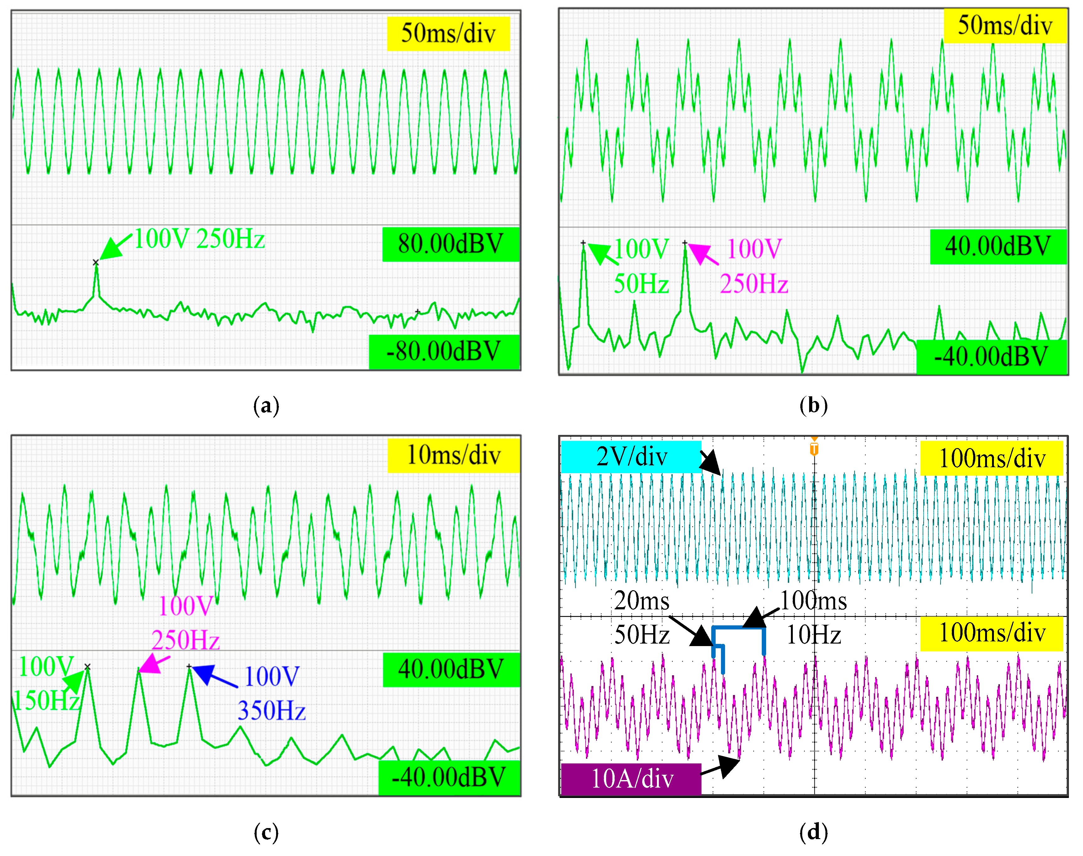
4. Experiment Results

In order to verify the correctness of the theoretical analysis and the feasibility of the design scheme of the MW multifunctional power grid simulator, an experimental platform of a 2MW power grid simulator was built and the corresponding experimental verification was carried out. The platform relies on the National Key R&D Project; Figure 9 is a brief introduction of the whole project. The key technology is the generator-type power grid simulator with complex operating conditions mentioned in this paper. The demonstration project establishes a configuration visualization master control platform shown in Figure 10 based on LabVIEW, and realizes the terminal control of the whole demonstration system through ModBus industrial communication protocol. The experimental platform hardware photos are shown in Figure 11; among them the digital processing chip of the system adopts the TMS320LF283xx produced by Texas Instruments Company located in Dallas, TX, USA.

The power network simulator is power and electronic equipment with a real power grid. The virtual synchronous generator technology is used to simulate the high-order electromagnetic transient characteristics of a synchronous generator and support the operation of the whole system. The output voltage and current waveform of the 2MW grid simulator with dropping control and inertial control characteristics is shown in Figure 12. When the sag coefficient m = 1 p.u., the system frequency decreases by 0.2 Hz; when the inertia coefficient J = 1 p.u., the system recovery time is 2 s.

The SC100 energy storage converter can adaptively switch current source and voltage source control mode to the 2MW grid simulator and finally solve the problem of weak grid instability of the current source converter. Figure 13 and Figure 14 show the voltage and current waveform of SC100 full power current source and voltage source connected to the 2MW grid simulator. As can be seen from the figure, SC100 energy storage inverters are merged into the power grid simulator in the form of current source and voltage source at t₁ and t₂, respectively. After a period of adjustment, the grid connection can be successfully completed.

The harmonic generator is realized by high-power density inverters. A hybrid topology composed of new wide bandgap devices and traditional devices is used to realize the single-machine power of inverters greater than 100 kW, power density greater than 1.0 W/cm³, and efficiency greater than 99%. At the same time, phase-change thermal siphon cooling technology is used to ensure the stable and safe operation of the inverters.

Figure 15a–c respectively show the output of 100 V fifth harmonic voltage waveform; 100 V 50 Hz fundamental wave and 100 V 250 Hz harmonic combined voltage waveform; and 100 V 150 Hz, 100 V 250 Hz, and 100 V 350 Hz harmonic combined voltage waveform of the 2MW multifunctional power grid simulator when no load occurs. From the FFT analysis results in the figure, it can be seen that the 2MW multifunctional power grid simulator can output 100 V 150 Hz, 100 V 250 Hz, and 100 V 350 Hz harmonic combined voltage waveform without load. To simulate the output of specified frequency and amplitude of single or multiple specified harmonic voltage waveforms, Figure 15 shows spectrum analysis of the produced signals. However, the spectrum should be theoretically with discrete values (only the fundamental and harmonics), but the graphs (a), (b), and (c) show continuous spectrum with some peaks; however, with a series of odd harmonic voltages, such big noise in the spectrum is mainly caused by the dead time [24,25,26].

In the full bridge converter composed of full control devices, the dead time must be added to the upper and lower switch signals of the same bridge arm to prevent the switch device from burning due to the through fault of the bridge arm. The existence of this dead time will make the actual output voltage of the inverter deviate from the ideal voltage.

As shown in Figure 16, if the dead time is added to the gate level drive of the upper and lower tubes of the bridge arm, such as the delay opening t_d, the output voltage of the inverter bridge will be different from the ideal command voltage, which is related to the current flow direction. As shown in Figure 17a,b, when the current flows to the middle point O of the bridge arm, during the period when T₃ is normally closed and T₄ is delayed to open, D₁ and D₄ will continue to flow, and the output voltage of the bridge arm is equal to Vdc, that is to say, the output voltage is the same as the ideal command voltage in this dead time. In the second dead time period (i.e., when T₁ is normally closed and T₂ is delayed to open), D₁ and D₄ will continue to flow, and the output voltage of the bridge arm is equal to V_dc. During this period, the output voltage should be zero, which is the error caused by the dead time voltage. In the first T_d, the output voltage is equal to zero, and the deviation from the ideal U_inv is −V_dc.

The error caused by dead time voltage exists in every switching cycle. When analyzing the dead time effect, the average voltage of dead time voltage in a power frequency cycle can be approximately used to describe it. It can be seen from the above analysis that the polarity of the dead time average voltage is opposite to that of the current.

$$U_{dead}=-\frac{t_d}{T_s}{V}_{dc}sgn(i_L)$$

(15)

Therefore, it can be represented by a square wave superimposed on the ideal sinusoidal output voltage, which is opposite to the polarity of the current. By Fourier decomposition of this square wave, a series of odd harmonic voltages are obtained as follows:

$$U_{dead}(t)=\frac{4t_d{V}_{dc}}{\pi T_s}{\displaystyle \sum _{k=1,3,5\dots }^{\infty }\frac{1}{k}}\sin (k{w}_{0}t)$$

(16)

One idea to improve the quality of voltage waveform is to add a harmonic controller which can suppress the corresponding times. Resonance control and repetitive control have similar frequency characteristics, which can generate infinite gain at a specific frequency, so that the voltage instructions at these frequencies can be tracked without static difference or the disturbance at these frequencies can be fully suppressed. Therefore, two kinds of control are widely used to eliminate the specific subharmonic components.

Figure 15d is the output voltage and current waveform of a 2MW multifunctional power grid simulator connected to the stator terminal of a doubly fed machine. From the current waveform, the output current contains 50 Hz fundamental wave and 10 Hz noncharacteristic subharmonics. It is well known that the subsynchronous oscillation (SSO) caused by noncharacteristic subharmonics plays a very important role in motor research, but the existing research is very important. The multifunctional power grid simulator proposed in this paper can provide the necessary research environment for the study of subsynchronous oscillation by giving the frequency and amplitude of the noncharacteristic harmonic voltage below 50 Hz.

Figure 18a is the working voltage waveform of the 2MW power grid simulator with 500 kW inverter load output 315 V 50 Hz; Figure 18b–d are the voltage waveform of power grid simulator with 500 kW inverter output fundamental 315 V and fifth harmonic 25 V combination; output fundamental 315 V, ninth harmonic 15 V, and fourteenth harmonic 15 V combination; and output fundamental 315 V, fifth harmonic 15 V, ninth harmonic 15 V, fourteen harmonic 1 V, respectively. Figure 18 verifies that the 2MW grid simulator can work normally with the inverter load, and provides the fundamental or harmonic combination test conditions for the inverter load.

Figure 19a–c show the output voltage waveforms of the power network simulator when the simulated fundamental resistance is 10 Ω, the inductance of the fundamental line is 0.03 H, and the resistance of the fundamental line is 0.03 H. Figure 19 d–f show the output voltage waveforms of the power network simulator when the simulated fifth harmonic resistance is 10 Ω, the fifth harmonic inductance is 0.03 H, and the fifth harmonic line resistance-inductance is 10 Ω + 0.03 H. According to the experimental waveforms and data, the errors of impedance simulation can be calculated and analyzed as shown in

Table 1. Error analysis of line impedance simulation.

Error	Fundamental Wave	Fifth Harmonic
Resistance	1.1%	1.2%
Inductance	1.2%	0.7%
Resistance–Inductance	0.6%	0.1%

.

Constant impedance, constant current, and constant power modes are adopted. The corresponding coefficients are shown in

Table 2. ZIP load model parameters.

Simulation Parameters	Figure	Simulation Parameters	Figure
$p_1$	0.2	$q_1$	0.2
$p_2$	0.2	$q_2$	0.2
$p_3$	0.2	$q_3$	0.6
$k_{pf}$	1	$k_{qf}$	−1

. From Figure 20, it can be seen that the corresponding impedance, current, and power are almost as constant values. The rectifier side current is fed back to the DC source. The load does not actually consume energy, and the energy is only consumed in power electronic devices and transmission loops.

The experimental verification of the proposed MW multifunctional power grid simulator system with line impedance simulation is carried out from both steady and transient aspects, which fully proves the correctness, effectiveness, and flexibility of the proposed power grid simulator system scheme. Moreover, by setting the parameters of the upper computer control interface, various required power grid faults can be simulated.

5. Conclusions

This work has comprehensively described a multifunctional high-power grid simulator system. A detailed explanation about the hardware implementation has been provided. The control strategy of each part has also been described in detail. The main objective of the setup is to obtain experimental results which can confirm the validity of different control proposals.

• A novel topology for a megawatt high-power grid source simulator is proposed, which solves the problem of control bandwidth limitation in high-power grid simulator systems;
• A closed-loop control strategy using filter to separate harmonics and amplitude is proposed, which can effectively realize zero error harmonic voltage tracking;
• The functions of virtual line impedance simulation and arbitrary harmonic impedance simulation of the MW multifunctional power grid simulator system are realized. By adjusting the line impedance online, the problem of uneven power distribution in photovoltaic grid-connected systems can be solved, and the shortcomings of previous power grid simulators that only simulate ideal voltage sources are perfected.
• A constant-impedance, constant-current, and constant-power load model is adopted. The load does not actually consume energy, and the energy is only consumed in power electronic devices and transmission loops.

A complete experimental section has demonstrated the interesting and flexible behavior of the described grid simulator system, which fully proves the correctness, effectiveness, and flexibility of the proposed power grid simulator system scheme.

References

1. Miret, J.; García de Vicuña, J.; Guzmán, R.; Camacho, A.; Moradi Ghahderijani, M. A Flexible Experimental Laboratory for Distributed Generation Networks Based on Power Inverters. Energies 2017, 10, 1589. [Google Scholar] [CrossRef] [Green Version]
2. Adefarati, T.; Bansal, R.C. Integration of renewable distributed generators into the distribution system: A review. IET Renew. Power Gener. 2016, 10, 873–884. [Google Scholar] [CrossRef]
3. Kahrobaeian, A.; Mohamed, Y.-R. Interactive distributed generation interface for flexible micro-grid operation in smart distribution systems. Sustain. Energy IEEE Trans. 2012, 3, 295–305. [Google Scholar]
4. Montori, F.; Borghetti, A.; Napolitano, F. A Co-Simulation Platform for the Analysis of the Impact of Electromobility Scenarios on the Urban Distribution Network. In Proceedings of the 2nd International Forum on Research and Technologies for Society and Industry (RTSI 2016), Bologna, Italy, 7–9 September 2016; pp. 1–6. [Google Scholar]
5. Commission Regulation (EU). 2016/631 of 14 April 2016 Establishing a Network Code on Requirements for Grid Connection of Generators (Text with EEA relevance) C/2016/2001, OJ L 112, 27.4.2016. pp. 1–68, (BG, ES, CS, DA, DE, ET, EL, EN, FR, HR, IT, LV, LT, HU, MT, NL, PL, PT, RO, SK, SL, FI, SV). Available online: http://eur-lex.europa.eu/legal-content/EN/TXT/?uri=OJ:JOL_2016_112_R_0001 (accessed on 22 November 2019).
6. IEEE. 1547TM Standard for Interconnecting Distributed Resources with Electric Power Systems. Available online: http://www.doc88.com/p-74459601668.html (accessed on 22 November 2019).
7. Yanfeng, M.; Shuju, H.; Xu, L. Research on Wind Power Simulation Technology Applied to Power System Dynamic Simulation Test System. Trans. China Electrotech. Soc. 2016, 31, 130–137. [Google Scholar]
8. Parameters of Non-Exhaustive Requirements ENTSO-E Guidance Document for National Implementation for Network Codes on Grid Connection, ENTSO-E, 16 November 2016. Available online: https://docstore.entsoe.eu/Documents/Network%20codes%20documents/NC%20RfG/161116_IGD_General%20guidance%20on%20parameters_for%20publication.pdf (accessed on 22 November 2019).
9. Bründlinger, R.; Arnold, G.; Schäfer, N.; Schaupp, T.; Graditi, G.; Adinolfi, G. Implementation of the European Network Code on Requirements for Generators on the European national level. In Proceedings of the Solar Integration Workshop, Stockholm, Sweden, 15–19 October 2018. [Google Scholar]
10. Network Code for Requirements For Grid Connection Applicable To All Generators Frequently Asked Questions, 19 June 2012. Available online: https://www.entsoe.eu/fileadmin/user_upload/_library/consultations/Network_Code_RfG/120626_-_NC_RfG_-_Frequently_Asked_Questions.pdf (accessed on 22 November 2019).
11. ENTSO-E Connection Network Codes Implementation Website. Available online: https://docs.entsoe.eu/cnc-al/ (accessed on 22 November 2019).
12. Li, S.; Qin, S.; Wang, R.; Li, Q.; Chen, C. Study on grid adaptability testing methodology for wind turbines. J. Mod. Power Syst. Clean Energy 2013, 1, 81–87. [Google Scholar] [CrossRef] [Green Version]
13. Zhang, R.; Cardinal, M.; Paul, S.; Dame, M. A Grid Simulator with Control of Single-phase Power Converters in D-Q Rotating Frame. In Proceedings of the 2002 IEEE 33rd Annual IEEE Power Electronics Specialists Conference, Cairns, Australia, 23–27 June 2002; pp. 1431–1436. [Google Scholar]
14. Guo, X.; Zhang, X.; Wang, B.; Wu, W.; Guerrero, J.M. Asymmetrical grid fault ride-through strategy of three-phase grid-connected inverter considering network impedance impact in low-voltage grid. IEEE Trans. Power Electron. 2014, 29, 1064–1068. [Google Scholar] [CrossRef] [Green Version]
15. Hu, S.J.; Li, J.L.; Xu, H.H. Review of voltage sag generatator for wind power. Power Syst. Autom. Equip. 2008, 21, 101–103. [Google Scholar]
16. Dingguo, W.; Zhuo, C.; Weizheng, Y.; Gang, L. Analysis of grid-connected PV inverter low voltage ride through testing scheme. Power Syst. Prot. Detect. 2014, 42, 143–147. [Google Scholar]
17. Ying, W.; Li, J.; Liu, F. Research of Multi-Functional Grid Simulator. Power Electron. 2011, 45, 29–34. [Google Scholar]
18. Xu, H.; Zhang, W.; Hu, J.; Zhou, P.; He, Y. Design of a Programmable Grid-Fault Emulating Power Supply. Trans. China Electrotech. Soc. 2012, 27, 91–97. [Google Scholar]
19. Wang, X.; Li, Y.W.; Blaabjerg, F.; Loh, P.C. Research on synchronous voltage source control strategy based on composite virtual impedance in microgrid. Mod. Electr. Power 2014, 2, 60–65. [Google Scholar]
20. Ma, T.; Jin, X.; Liang, J. Hybrid virtual impedance control strategy for islanding mode microgrid converter. Trans. China Electrotech. Soc. 2013, 28, 304–312. [Google Scholar]
21. Bian, X. Simulation and analysis of fundamental current extraction algorithm based on Simulink. Electr. Eng. 2016, 17, 51–55. [Google Scholar]
22. Kundur, P. Power System Stability and Control; McGrawHill: New York, NY, USA, 1994. [Google Scholar]
23. Wang, J.; Yang, L.; Ma, Y.; Wang, J.; Tolbert, L.M.; Wang, F.F.; Tomsovic, K. Static and dynamic power system load emulation in converter-based reconfigurable power grid emulator. Energy Convers. Congr. Expo. 2015, 31, 3239–3251. [Google Scholar]
24. Gong, R.; Shen, C. Analysis of dead band time on the influence of three-phase SPWM inverter output voltage low harmonic. Sci. Technol. Vis. 2014, 27, 22. [Google Scholar]
25. Li, R. Research on the Method of Current Harmonic Suppression in Single-Phase Grid-Connected Inverters. Master’s Thesis, Huazhong University of Science and Technology, Wuhan, China, January 2012. [Google Scholar]
26. Kong, D.; Liu, Y.; Gao, L.; Zhang, Q. Harmonic suppression method of grid connected inverter with virtual harmonic impedance. J. Heilongjiang Inst. Technol. 2015, 29, 3–5. [Google Scholar]
Figure 1. Multifunctional high-power grid source simulator system: (a) schematic; (b) topology.
Energies 12 04657 g001aEnergies 12 04657 g001b
Figure 2. Control strategy of the voltage source Eg.
Energies 12 04657 g002
Figure 3. Amplitude closed-loop control strategy of the harmonic generator.
Energies 12 04657 g003
Figure 4. Bode of amplitude closed-loop control method.
Energies 12 04657 g004
Figure 5. Amplitude closed-loop control simulation waveform of three harmonics combination.
Energies 12 04657 g005
Figure 6. Control diagram of the fundamental and harmonic line impedance simulation: (a) control diagram of the fundamental line impedance simulation; (b) control diagram of the harmonic line impedance simulation.
Energies 12 04657 g006
Figure 7. Control strategy of the ZIP load.
Energies 12 04657 g007
Figure 8. Emulated ZIP model inputs and outputs relationship.
Energies 12 04657 g008
Figure 9. Brief introduction of National Key R&D Program system test platform.
Energies 12 04657 g009
Figure 10. Configuration visualization master control platform based on LabVIEW.
Energies 12 04657 g010
Figure 11. Experimental platform of National Key R&D Program system.
Energies 12 04657 g011
Figure 12. Output voltage and current waveform of 2MW grid simulator with dropping control characteristic.
Energies 12 04657 g012
Figure 13. Voltage and current waveform of SC100 full power current source connected to grid.
Energies 12 04657 g013
Figure 14. Voltage and current waveform of SC100 full power voltage source connected to grid.
Energies 12 04657 g014
Figure 15. Fundamental and characteristic or noncharacteristic harmonic combination voltage of grid simulator without load: (a) no-load output of the simulator 100 V 250 Hz voltage; (b) simulator no-load output 100 V 50 Hz and 100 V 250 Hz combined voltage; (c) simulator no-load output 100 V 150 Hz, 100 V 250 Hz and 100 V 350 Hz combined voltage; (d) the simulator output 50 Hz fundamental wave and 10 Hz noncharacteristic harmonic voltage.
Energies 12 04657 g015
Figure 16. Simplified diagram of single-phase inverter bridge.
Energies 12 04657 g016
Figure 17. Dead time voltage analysis: (a) first dead band; (b) second dead band.
Energies 12 04657 g017
Figure 18. Fundamental and harmonic combination voltage of grid simulator with an inverter load: (a) simulator with 500 kW inverter load output 100 V 50 Hz voltage; (b) load output of simulator with 500 kW inverter 315 V 50 Hz and 25 V 250 Hz voltage combination; (c) voltage combination of 315 V 50 Hz, 25 V 250 Hz, and 15 V 700 Hz load output of simulator with 500 kW inverter; (d) load output of simulator with 500 kW inverter 315 V 50 Hz, 15 V 250 Hz, 15 V 450 Hz, and 10 V 700 Hz voltage combination.
Energies 12 04657 g018
Figure 19. Fundamental and fifth harmonic with resistance and inductance impedance simulation voltage waveform: (a) output voltage and current waveform of imitating circuit at resistance 10 Ω; (b) output voltage and current waveform of imitating circuit inductance at 0.03 H; (c) output voltage and current waveform of imitating line resistance–inductance load at 10 Ω + 0.03 H; (d) output voltage and current waveform of imitating fifth harmonic resistance at 10 Ω; (e) output voltage and current waveform of imitating fifth harmonic circuit inductance at 0.03 H; (f) output voltage and current waveform of imitating fifth harmonic line resistance–inductance load at 10 Ω + 0.03 H.
Energies 12 04657 g019aEnergies 12 04657 g019b
Figure 20. DC voltage, current, and power of ZIP load model: (a) DC output power of ZIP load; (b) DC output power of ZIP load; (c) DC output power of ZIP load.
Energies 12 04657 g020