Article

Comparative Assessment of Priority Listing and Mixed Integer Linear Programming Unit Commitment Methods for Non-Interconnected Island Systems

by
Georgios N. Psarros
* and
Stavros A. Papathanassiou
School of Electrical and Computer Engineering, National Technical University of Athens (NTUA), 15780 Athens, Greece
*
Author to whom correspondence should be addressed.
Energies 2019, 12(4), 657; https://doi.org/10.3390/en12040657
Submission received: 27 December 2018 / Revised: 29 January 2019 / Accepted: 14 February 2019 / Published: 18 February 2019

Abstract

:
The generation management concept for non-interconnected island (NII) systems is traditionally based on simple, semi-empirical operating rules dating back to the era before the massive deployment of renewable energy sources (RES), which do not achieve maximum RES penetration, optimal dispatch of thermal units and satisfaction of system security criteria. Nowadays, more advanced unit commitment (UC) and economic-dispatch (ED) approaches based on optimization techniques are gradually introduced to safeguard system operation against severe disturbances, to prioritize RES participation and to optimize dispatch of the thermal generation fleet. The main objective of this paper is to comparatively assess the traditionally applied priority listing (PL) UC method and a more sophisticated mixed integer linear programming (MILP) UC optimization approach, dedicated to NII power systems. Additionally, to facilitate the comparison of the UC approaches and quantify their impact on systems security, a first attempt is made to relate the primary reserves capability of each unit to the maximum acceptable frequency deviation at steady state conditions after a severe disturbance and the droop characteristic of the unit’s speed governor. The fundamental differences between the two approaches are presented and discussed, while daily and annual simulations are performed and the results obtained are further analyzed.

1. Introduction

Isolated island grids are power systems present particular characteristics compared to larger, robust continental power systems. They are generally systems of limited size (with peak demand typically not exceeding some hundreds of MWs for the largest of them [1,2]) and low inertia, lacking interconnections to large mainland grids, being thus vulnerable to disturbances, such as the unexpected loss of generation, be it thermal or RES units [3,4]. Hence, the integration of intermittent renewables is severely limited by security considerations, as well as other technical constraints, related to the characteristics and management of conventional generation [5,6,7,8,9,10].
In non-interconnected islands (NIIs), advanced generation management concepts and tools are today considered essential both to ensure maximum RES exploitation and to safeguard security of operation and supply of load demand [2]. Still, the generation management practices currently applied in many NII systems are based predominantly on traditional dispatch methods that come from the era before the massive development of renewables [11,12]. They are usually based on simplified security criteria, such as the total spinning reserve of the system, without distinguishing reserves types according to their deployment time [13,14], while unit commitment is typically performed through priority listing (PL) techniques, i.e., merit order classification of available units. This is still the common practice in small and medium-sized islands ([1,2]), where Energy Control Centres (ECCs) are yet to be installed. Modified versions of the PL unit commitment (UC) approach have been recently proposed in the literature [13,15] for island power systems, to deal with renewable-based dispatchable stations and increase the effectiveness of the method.
Such practices, involving empirical UC and economic-dispatch (ED) decisions taken during real-time operation, are hardly suitable to support the future operation of the systems, especially under high RES penetration conditions. More sophisticated UC-ED methods have already been proposed in the literature and in some cases applied in prototype, real-world ECCs for NII systems [16], based on optimization techniques, such as the state-of-the-art mixed integer linear programming (MILP) approach [17,18,19,20,21]. Alternative UC methodologies for application in isolated power systems are described in Reference [22], providing insight to the available techniques to be adopted for generation management in NIIs. In References [23] and [24] a deterministic MILP-UC approach is proposed elaborating frequency constraints to determine the levels of systems reserves. The operation of an island system utilizing MILP-based UC under various wind and photovoltaic (PV) penetration scenarios is also examined in Reference [25]. A stochastic MILP-UC is proposed in References [26] and [27] to evaluate the risk of scheduling decisions under uncertainty and to quantify the levels of load-following reserves in autonomous power systems, respectively. A MILP multi-stage robust optimization method based on Bender’s decomposition technique is investigated in Reference [28] for a small Chinese island, to deal with high RES penetration levels. A coordinated generation management scheme is presented in Reference [29] for the Greek NII power systems and a deterministic MILP-based detailed mathematical formulation of the generation scheduling problem for island systems is proposed for implementation in the ECCs of Greek islands. A more complex MILP-UC method is proposed in Reference [30] to take advantage of the limited underloading capability of base-load units during low-demand hours for achieving economic and feasible UC patterns. Overall, MILP-based UC methods for islands dominate recent literature, being considered suitable for implementation in real-world island ECCs.
The motivation for this work originates from the topical and recurring question of the benefits anticipated from introducing advanced generation management practices in small island systems and whether those benefits outweigh the additional complexity and resources required. Although several papers are available dealing either with simple PL-UC methods or with more sophisticated optimization-based UC methods, their systematic comparison, based on quantitative evidence and taking account of the different objectives to be achieved, is missing in the literature. Therefore, in this paper, the traditional PL-UC approach and a comprehensive MILP optimization-based UC method are implemented and comparatively assessed via simulation for two realistic study-case islands, expanding the work presented in Reference [31]. The mathematical formulation of both methods is presented, while their fundamental differences are identified and highlighted. The typical daily UC pattern is analyzed for both UC alternatives, while annual results are also presented to evaluate their performance in terms of system security, generation cost and RES penetration levels, for a medium and a large-sized island.
An additional contribution of this paper concerns the quantification of primary reserves capabilities of dispatchable units in terms of the droop settings of their speed governors and the acceptable system frequency deviation limits. The established correlation is incorporated in the MILP-UC formulation, transforming it into a frequency constrained problem. The proposed approach allows for an objective comparison of the alternative UC approaches in terms of achieved system security, by quantifying anticipated under-frequency levels following a severe loss of generation disturbance.
The remaining of this paper is organized as follows: The mathematical formulation of the two UC variants under evaluation is described in Section 2 and their differences are discussed. The study-case island systems are presented in Section 3. Daily and annual analysis results are discussed in Section 4 for a variety of scenarios, while the main conclusions are summarized in Section 5.

2. Unit Commitment Variants

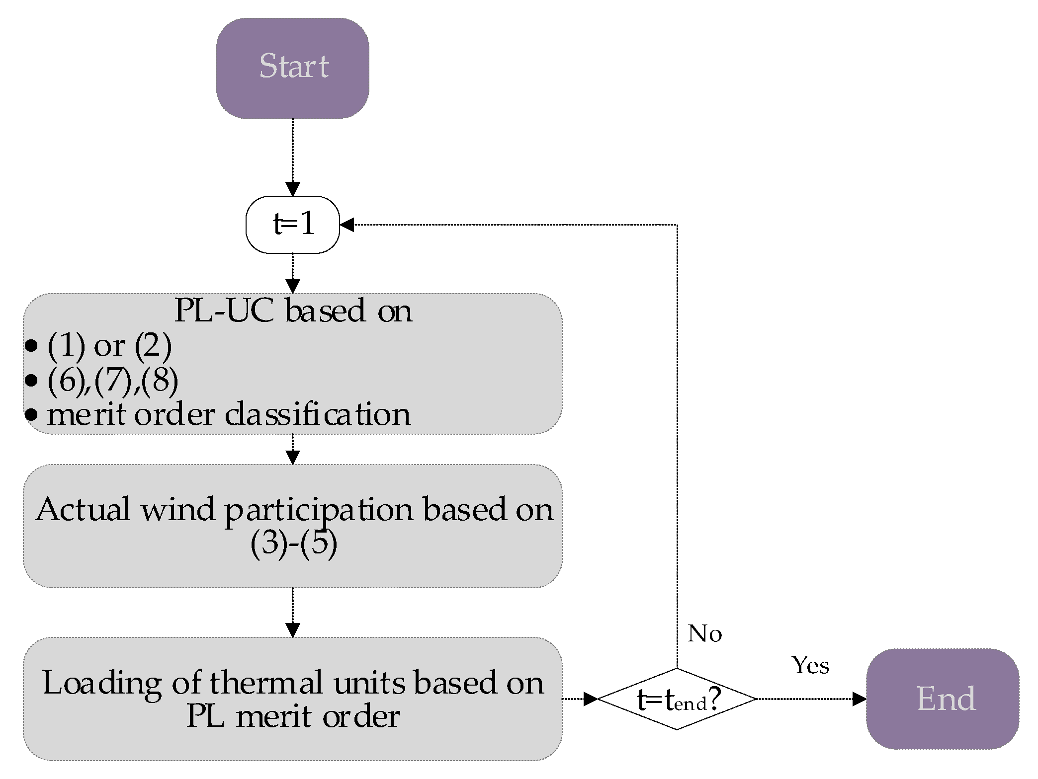
2.1. Priority Listing UC

The PL-UC variant approximates the standard generation scheduling practice, adopted in small and medium-sized NIIs without ECCs, where unit commitment is usually performed based on empirical policies, utilizing a merit order classification of available thermal units.
In the PL-UC method, the commitment order of conventional units is predominantly based on simple economic criteria, where the larger and cheaper units are usually prioritized compared to smaller or more expensive ones, although technical and security constraints may also be taken into account. Unit commitment decisions satisfy only fundamental constraints, such as the active power equilibrium. In the simplest form of the active power equilibrium Equation (1), the production of committed thermal units should equal the load demand per examined time interval, t. Variable x e n s , t , representing the energy not served, is also maintained in Equation (1) for cases where capacity adequacy issues exist in the island system. Small, distributed PV generation is effectively embedded to the load, not being subject to power limitations and curtailments [6], while wind generation is not accounted for, due to the lack of necessary forecasting and management tools.
u P u , t + x e n s , t = P L , t
An improved PL-UC approach would take into account an initial estimate of anticipated wind production. In this case, commitment of thermal units and load dispatch for time interval t is subject to Equation (2), where a level of anticipated wind generation P w , t e is taken into account.
u P u , t + P w , t e + x e n s , t = P L , t
Accountable wind generation, P w , t e , is estimated based on anticipated wind production, possibly limited to reflect security and dependability concerns; it represents the credit attributed to wind power at the UC stage with the PL formulation. Note that Equation (2) becomes equivalent to Equation (1) for P w , t e = 0 , i.e., when no credit can be given to wind power, as would be the case in very small systems.
Actual wind generation at t is given by Equation (3), determined by available wind power, limited by the minimum loading, Equation (4), and dynamic, Equation (5), limitations of conventional units, discussed in References [5,29,32]. The empirical coefficient lw represents in principle the fraction of wind generation that can be lost during operation and therefore needs to be covered by fast operating reserves, as discussed in References [7,29]. For the simplified PL-UC approach, where reserves types are not distinguished according to their deployment time, lw should be quantified more conservatively, so as to further incorporate wind power forecasting errors and variability.
P w , t a = min { P w , t M L , P w , t D , P w , t }
P w , t M L = P L , t u P u min
P w , t D = c D P L , t l w
The power output of each thermal unit is defined by Equation (6) accounting for Equation (2) and the assumed merit order classification. When online, a unit’s loading should not violate its technical minimum and maximum loading level. When a unit is offline, its power output equals to zero.
P u , t { P u max P u min   o n l i n e = 0         o f f l i n e
The operating reserves policy adopted for the PL-UC variant relies only on system spinning reserve, a common practice adopted by NII system operators [13,29]. Constraint (7) estimates the conventional capacity to be committed, so that a spinning reserve of at least ε(%) (e.g., ε = 15%) of net demand to be maintained. In order to ensure that system spinning reserves suffice to meet the loss of largest generator (G-1) criterion, constraint (8) should apply as well.
u P u max ( 1 + ε ) P L , t
u P u max P L , t + max u { P u max }
The PL-UC is simulated according to the flowchart of Figure 1. Initially, conventional units are committed based on their merit order classification, subject to Equation (1) or to Equation (2), depending on whether wind production is accounted for or not, as well as to constraints (7) and (8) to ensure the necessary reserves. Given the UC pattern, the actual wind participation is determined by Equations (3)–(5), while the final loading levels of online thermal units are then deduced based on their merit order. The entire process is repeated adopting an hourly time step, for the entire simulation period (one year).

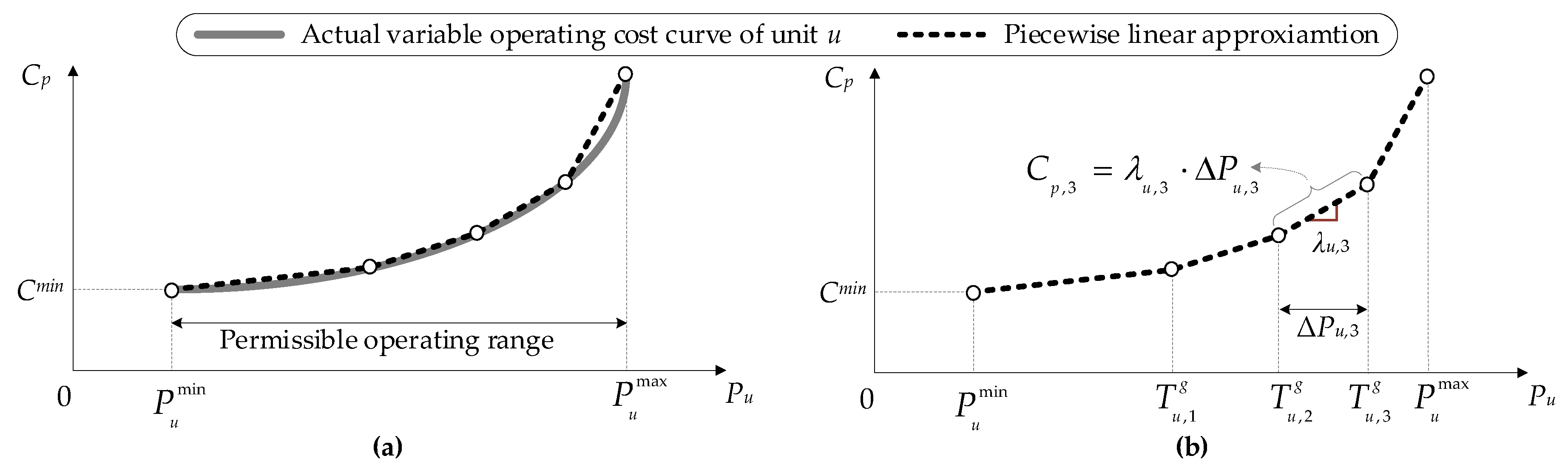
2.2. Deterministic MILP-Based UC

In this section the mathematical formulation of a MILP-based UC-ED optimization method is presented, as a more systematic and coordinated generation management for a NII system. The MILP optimization algorithm is based on Reference [29], aiming at minimizing NII system production cost and maximizing RES penetration, while guaranteeing secure operation via maintaining the required levels of active power reserves [33].
The objective function of the UC problem, given by (9), aims at minimizing the operating costs of conventional units (Cp), including start-up (Csu) and shut-down (Csd) costs [34,35], and maximizing RES penetration. The latter is achieved by assuming in (9) zero cost for RES energy and further penalizing RES curtailments, as discussed in Reference [29]. The leftmost term of (9) reflects the variable operating costs of conventional units, that are generally approximated by a quadratic function [36] (grey line in Figure 2a), that can be piecewise linearized (dashed-black line in Figure 2) and incorporated in the MILP via Constraints (10) to (12).
min { C p + C s u + C s d + C s l }
C p = t ( u ( C u min s t u , t + b ( λ u , b Δ P u , t , b ) ) )
P u , t = P u min s t u , t + b Δ P u , t , b
( T u , b g T u , b 1 g ) v u , b Δ P u , t , b ( T u , b g T u , b 1 g ) v u , b 1
The start-up and shut-down costs of thermal units are respectively defined by Equation (13) and Equation (14). The rightmost term of (9) is further expanded in Equation (15), incorporating the cost of all slack variables (x) introduced in the MILP constraints to ensure feasibility of solution in all cases, though properly appropriately penalized to minimize violations.
C s u = t u C u S U s u u , t
C s d = t u C u S D s d u , t
C s l = t ( κ e n s x e n s , t + u e κ e x u , t , e u p / d n )
Constraint (16) represents the active power equilibrium, including the amount of energy not served, x e n s , t . The logical status of commitment is imposed via Constraints (17) and (18). The binary variables of Constraints (17) and (18) are used for defining the start-up/shut-down decisions. Constraints (19) and (20) delimit the power output of each committed thermal unit by its ramping capabilities, while Constraints (21) and (22) bound the production levels of each unit, according to its maximum power output and its minimum loading. Fulfillment of reserves requirements is achieved through Constraints (23), (24) and (25), adopting the principle of reserves substitutability [37]. Finally, Constraint (26) ensures that the allocated reserves to each thermal unit do not exceed its capability per reserves type (primary, secondary, tertiary).
u P u , t + ( P w , t x w , t ) + x e n s , t = P L , t
s u u , t + s d u , t 1
s u u , t s d u , t = s t u , t s t u , t 1
P u , t P u , t 1 r u u s t u , t
P u , t 1 P u , t r d u s t u , t + P u max s d u , t
P u , t + e { p r , s r , t r } r u , t , e u p P u max s t u , t
P u , t e { p r , s r } r u , t , e d n P u min s t u , t
u r u , t , p r u p / d n + x u , t , p r u p / d n r r t , p r u p / d n
u e { p r , s r } r u , t , e u p / d n + x u , t , s r u p / d n e { p r , s r } r r t , e u p / d n
u e r u , t , e u p + x u , t , t r u p / d n e r r t , e u p
r u , t , e u p / d n R u , e s t u , t
The overall primary up reserves requirements of the system are defined according to Constraint (27), ensuring that sufficient reserves are collectively maintained by all units online to cater for the loss of the largest conventional unit or RES production. Additionally, Constraint (27) implicitly relates the maximum permissible wind penetration levels to the positive primary reserves capabilities of the online units. Secondary reserves requirements account for load and RES variability within a 5-min time window. Tertiary reserves requirements are calculated based on the variabilities of load and renewables for longer time scales (20 min), while accounting for forecasting errors as well. The quantification of secondary and tertiary reserves requirements is discussed more extensively in Reference [29].
r r t , p r u p = max ( max u { P u , t + r u , t , p r u p } , l w ( P w , t x w , t ) )
Actual wind power participation is calculated by Equation (3), as for the PL-UC method. However, the minimum loading and dynamic limitations are now described by Equations (28) and (29) respectively [29].
P W max , t M L = P L , t u P u min s t u , t
P W max , t D = u ( R u , p r s t u , t ) l w
The MILP-UC-ED is implemented in GAMS [38] using the CPLEX optimization solver [39], adopting a 24-h scheduling horizon with hourly dispatch time intervals.

2.3. Essential Differences Between the Examined UC Approaches

A first, rather obvious difference between the two UC approaches is related to the adopted fundamental unit commitment criterion: while in PL-UC a predetermined order governs the commitment priority of thermal units, in the MILP optimization the actual variable operating cost curves of the units are incorporated in the problem to achieve a more accurate representation of unit variable costs.
A subtler, but still fundamental, differentiation concerns the quantification of reserves requirements, which eventually impacts the eventual UC pattern and RES absorption capability of the system. In the MILP problem, reserves are classified according to their deployment time in primary (fast response) and then secondary and tertiary (Constraints (23)–(27)). On the other hand, with the PL-UC method only the aggregate spinning reserves of online thermal units are considered, in order to meet the requirements of the system (Constraints (7), (8)). The underlying assumption is that the entire operating range between the current loading level of an online unit and its maximum permissible power output ( P u max ), as in Figure 3a, is available to deploy in case of system disturbances, ignoring the associated time scales. In spite of its oversimplified nature, the concept of spinning reserves is quite commonly used for NII power systems [13,14,40], even in association with sophisticated UC approaches [28,41,42,43].
The hypothesis that the total amount of available spinning reserves can be released following a severe disturbance (e.g., tripping of a large generating unit) is obviously not valid. The dynamics of frequency regulation in power systems [44], related to the characteristics of prime movers and speed governors, are such that only a fraction of the available spinning reserves of generating units, hereinafter referred to as primary reserves, can be released right after the occurrence of a disturbance in the active power equilibrium of the system [4,24,45,46,47]. Ignoring the transient response of the system in the first few seconds following the disturbance (grey area of Figure 4a,b), the amount of active power released by each unit, before any secondary control corrective action takes place via automated generation control, is directly related to unit’s speed droop characteristic of Figure 4c, given by Equation (30). The primary reserves capability of each unit can be roughly derived from Equation (30), given the maximum acceptable frequency deviation at steady state conditions, Δ f s s , and the droop characteristic of the unit’s speed governor, symbolized by S (droop is generally symbolized by R, however, as R is already used for the reserves capabilities of thermal units, S will represent droop hereinafter instead of R).
R u , p r = Δ P u = Δ f s s / f 0 S u P u max
As illustrated in Figure 3, fast primary reserves are only a subset of the total available spinning reserves of a unit. Following primary regulation, additional reserves, denoted as secondary and tertiary reserves, can be released via slower external regulation action. The respective capabilities of each unit are determined by the ramp rate of the unit (MW/min) and the considered deployment times, e.g., 5 min and 20 min. The MILP-based UC-ED method recognizes this fundamental distinction between reserves types, implementing independent constraints for different reserves classes, whereas the PL-UC method adopts a simplified, aggregate spinning reserves approach.
As regards the participation of wind energy in the energy mix, it is always prioritized against conventional generation in both UC alternatives. However, wind curtailments are frequently inevitable in congested NII systems, whenever technical reasons do not allow the absorption of the total available wind power. Keeping that in mind, a further differentiation between the two UC variants is related to the limitations determining the participation of wind generation in the energy mix of the isolated power system, as explained in the following. The level of wind production that can be accommodated in the system at any operating interval is calculated based on two constraints: the minimum loading and the dynamic limitation. The former bounds wind penetration to avoid violating the minimum loading levels of online regulating units (Figure 5) and it is expressed in a similar manner in the PL- and MILP-UC methods (Equations (4) and (28), respectively). The latter represents the maximum amount of wind power that can be hosted by the system without posing a threat to its stability and it is implemented differently in for the examined UC alternatives. For the MILP-UC method, the dynamic limitation Equation (29) is directly related to the primary reserves capabilities of online thermal units. Thus, it is ensured that sufficient fast reserves are available to compensate any potential loss of wind generation, with no risk of unacceptable under-frequency events. Using Equation (30), Equation (29) can be reformulated as in Equation (31), in order to provide a quantitative relation between the dynamic limitation, the droop characteristics of the units and maximum system frequency deviation.
P W max , t D = Δ f s s f 0 u ( P u max S u s t u , t ) l w
As the PL-UC method does not distinguish between reserves types, the dynamic limitation cannot be implemented as described. Rather, Equation (5) is employed to calculate acceptable wind penetration levels as a fraction of system demand. This approach is common practice in island system analysis [5,48,49,50,51], as it constitutes a necessary compromise when the detailed characteristics of system units are not known [29]. Depending on the values of the empirical coefficients cD and lw, this simplified approach may over- or under-estimate the actual wind hosting capability of the system, with a potentially significant impact on its security.

3. Study-Case Systems

Two indicative NII systems with diversified characteristics will be examined as case studies. The first is a medium-sized island with a peak load demand of 80 MW and a load factor of 50%. The conventional generation portfolio of the island consists of seven heavy fuel oil (HFO) and seven light fuel oil (LFO) units, whose characteristics are presented in the Appendix A. Commitment of the five smallest LFO units is seasonal, limited to the summer peak demand period (July to September). The RES portfolio of the island includes 25 MW of wind farms (WFs), with an average capacity factor (CF) of ~32% before curtailments, as well as 15 MW of PVs with an annual yield of 1640 kWh/kWinstalled, which are embedded to the load. The second system has a peak demand of 220 MW and a load factor of 45%. It comprises 14 HFO units and 4 LFO units, as presented in the Appendix A. Renewables include 55 MW of WFs, with an average CF of ~37% before curtailments, and 36 MW of PVs with an annual yield of 1900 kWh/kWinstalled. For simulation purposes, a crude oil price of 80 $/bbl and a Euro to USD exchange rate of 1.25 $/€ are considered.

4. Results and Discussion

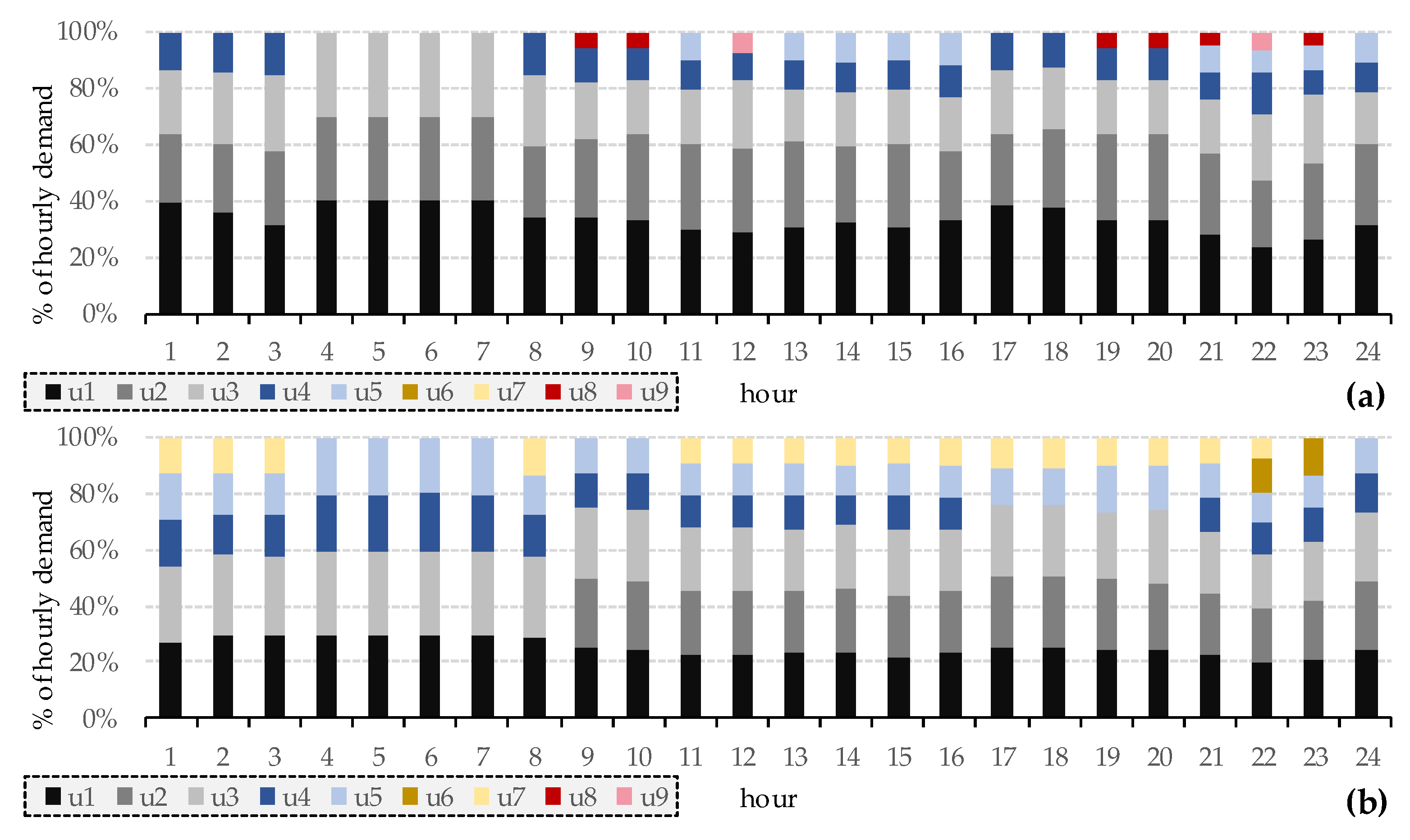
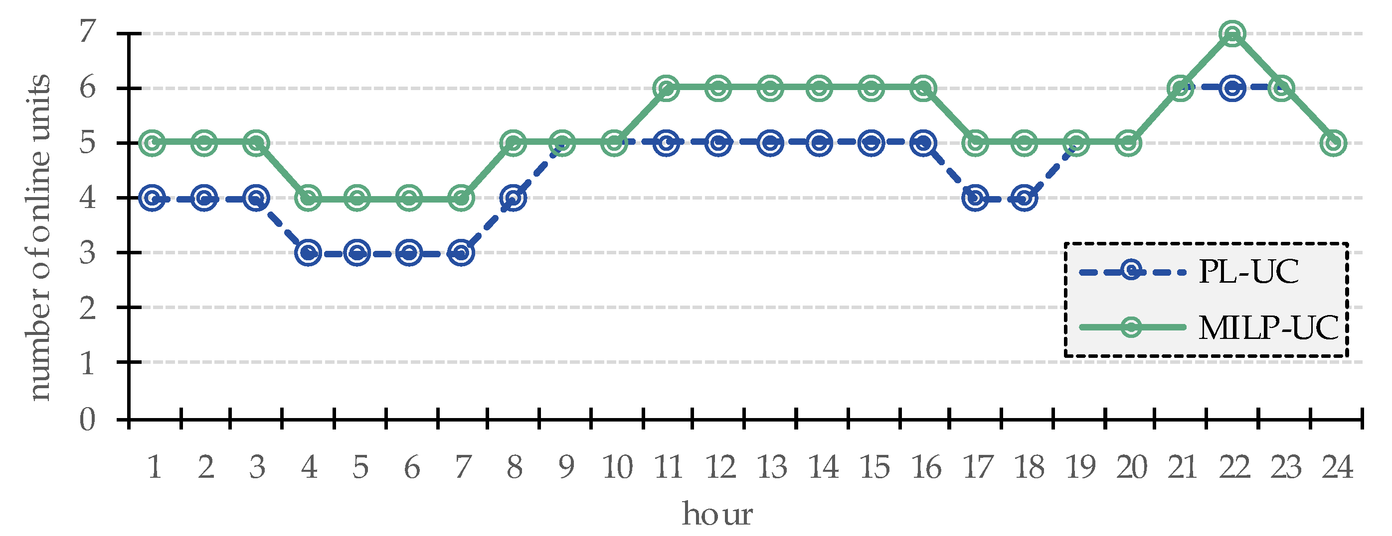
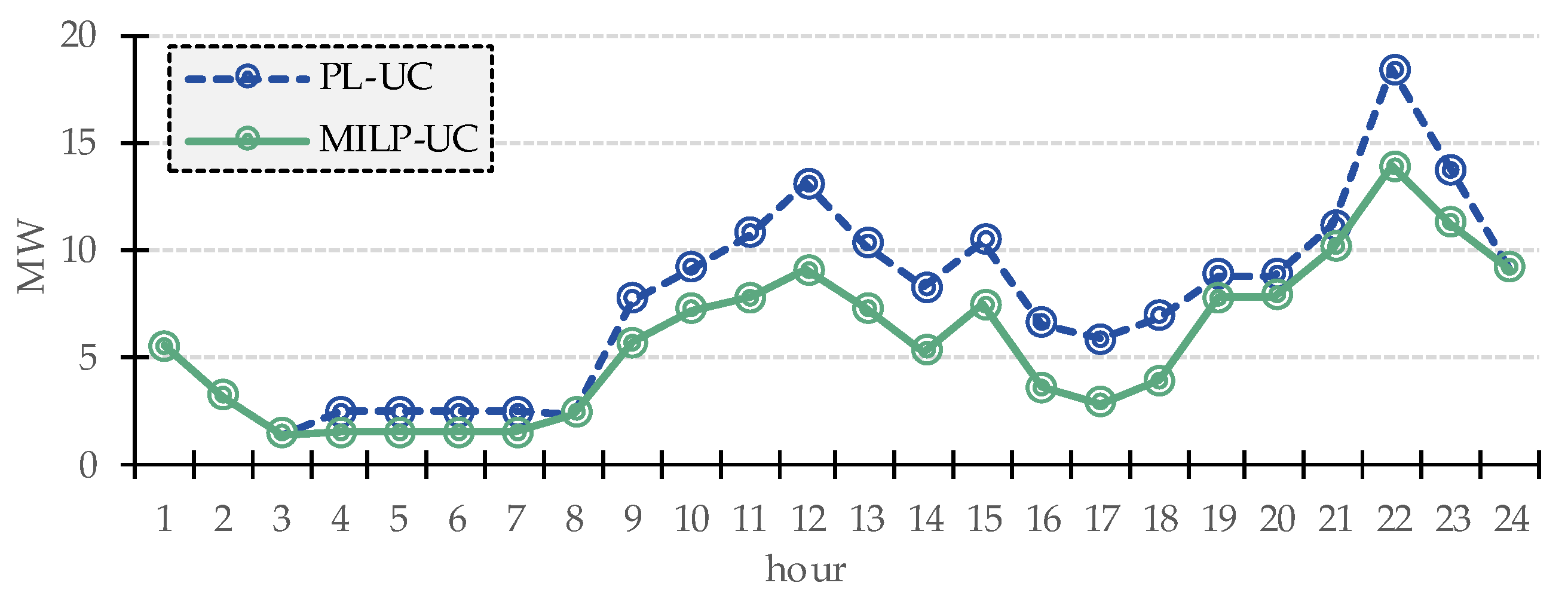
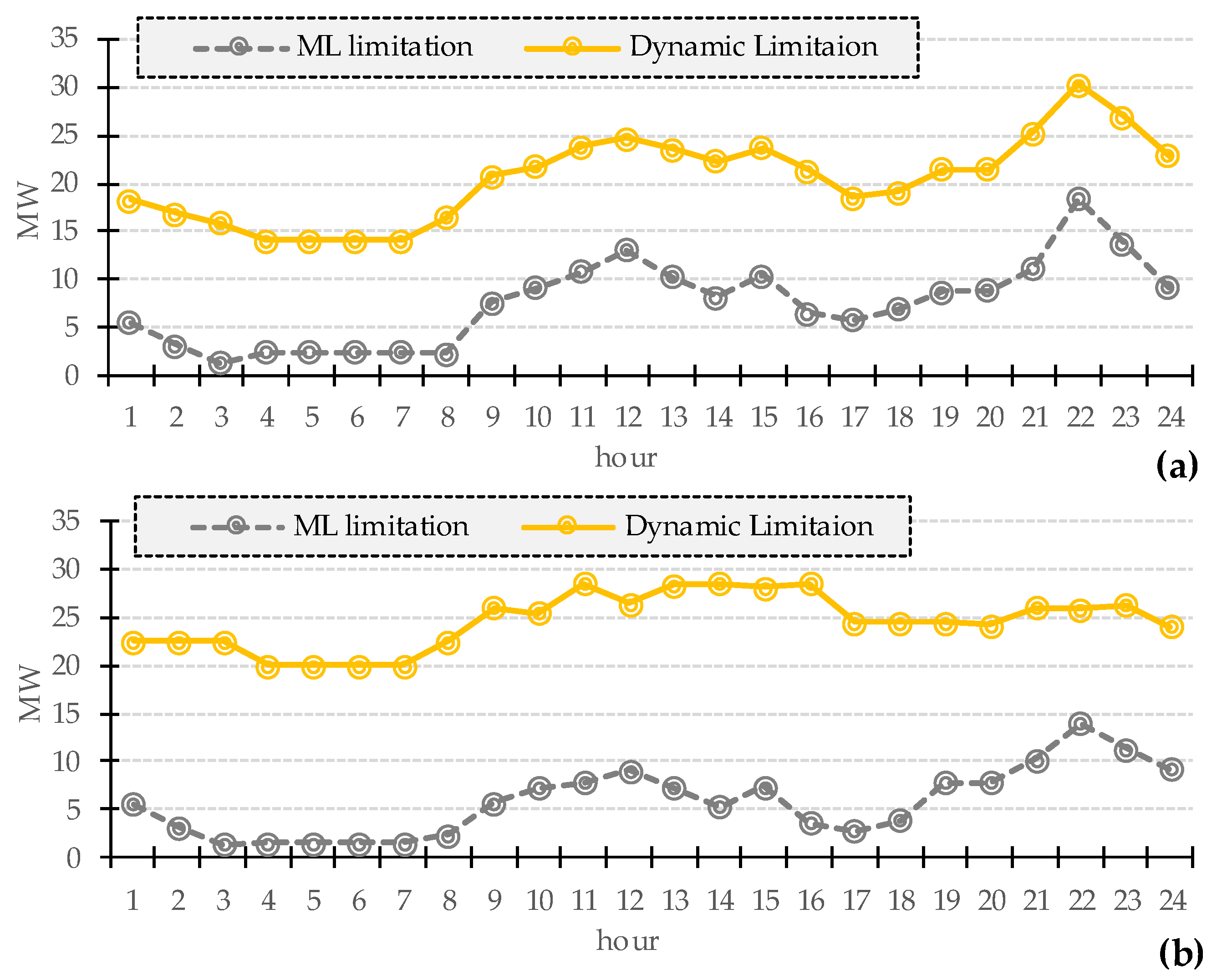
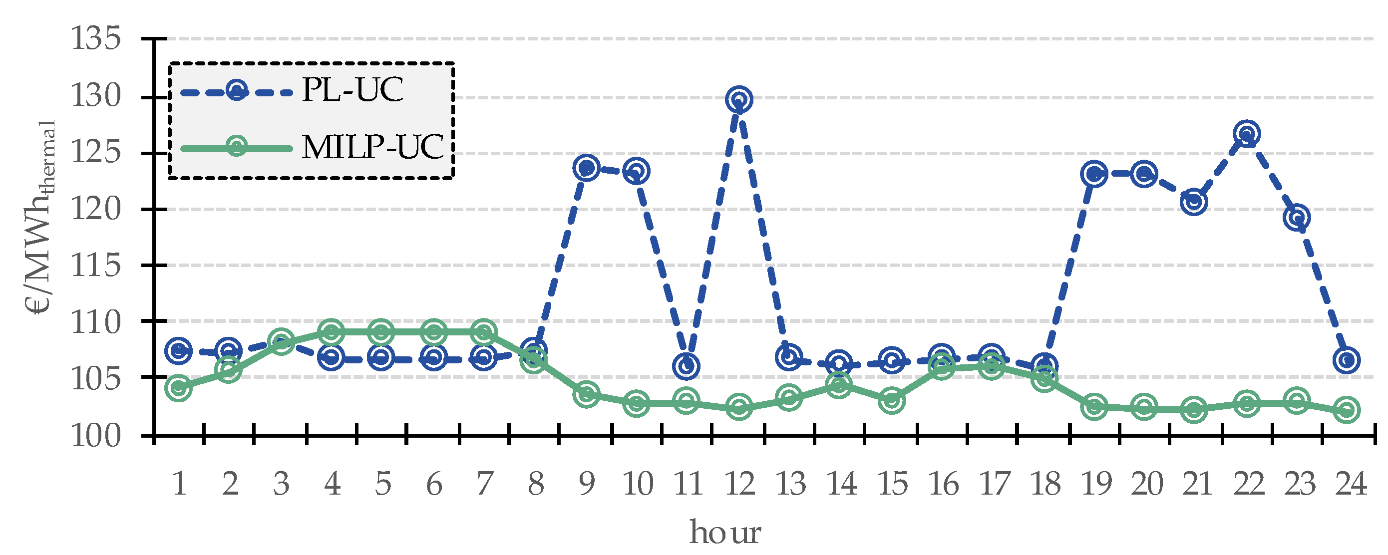
4.1. Operation of the Medium-Size Island System

4.1.1. Daily Operation without Wind Forecasting

Results obtained from the application of PL- and MILP-UC methods to the medium-sized island are first presented for an indicative low-demand day. To facilitate comparison, in both cases UC is performed without wind forecasting, to avoid changes in commitment patterns due to the substitution of thermal by wind production. Hence, the following two scenarios are examined:
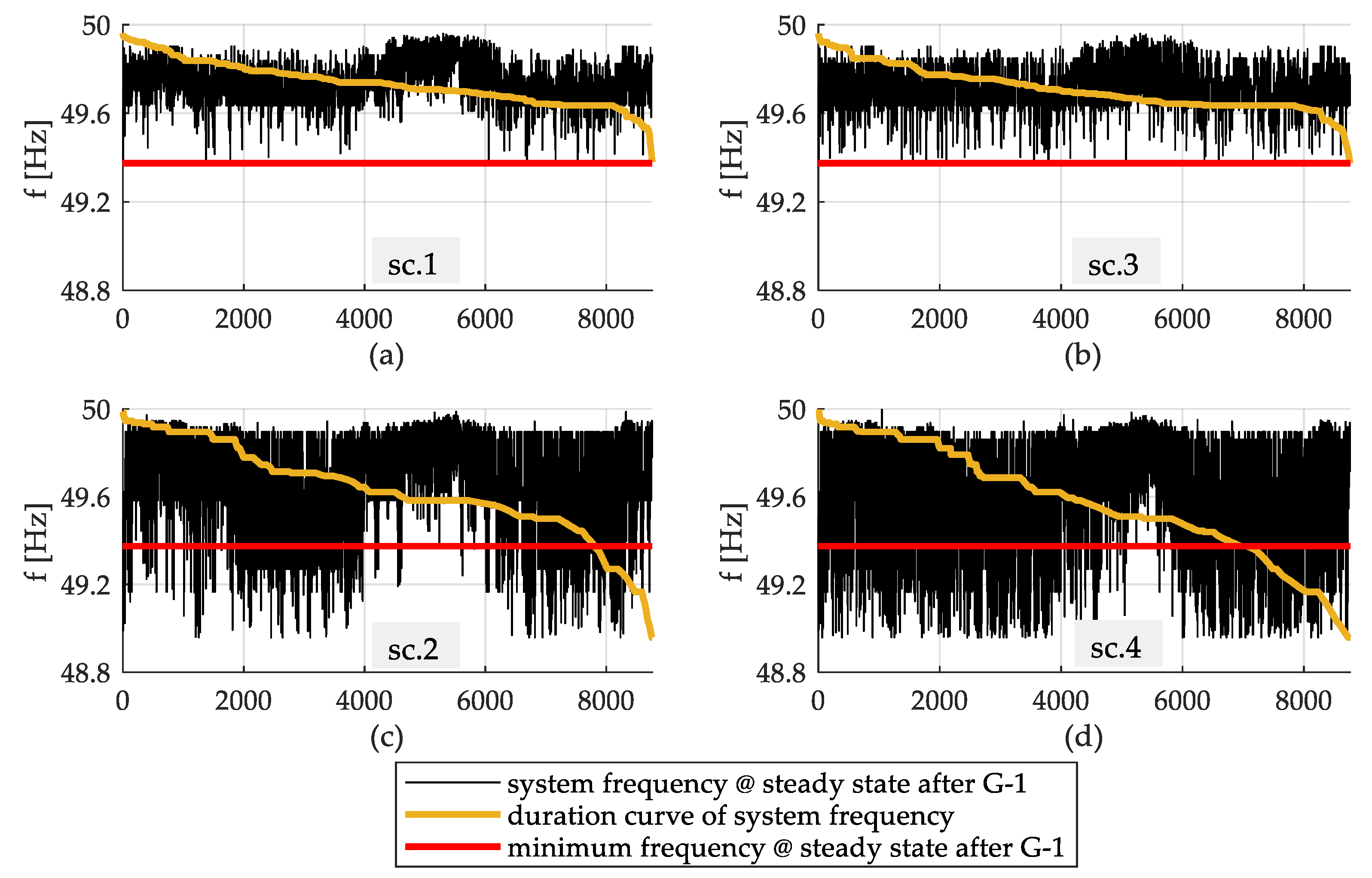
  • Scenario 1: MILP-UC without wind forecasting.
  • Scenario 2: PL-UC without wind forecasting.
The unit commitment derived by each model is depicted in Table 1, while the participation of each unit in meeting the hourly load demand is illustrated in Figure 6. White dots in Table 1 denote online units when PL-UC is applied, while black dots refer to committed units through the MILP-UC approach.
The largest and cheapest units of the system (HFO u1 to u3) are continuously committed by the PL-UC, based on the predefined commitment order (Table A1 and Table A2 of the Appendix A), covering at least 70% of hourly demand (Figure 6a). The expensive LFO units (u8-9, last in the priority list), capable of providing increased spinning reserves due to their low minimum loading (ML), are also frequently dispatched, in order to ensure the spinning reserves required to meet the G-1 criterion; nevertheless, these units are loaded as low as possible, as seen in Figure 6, to avoid further impact on system cost. The total spinning reserves available by all units always suffice to meet the G-1 criterion described by Constraint (8) (black solid line of Figure 7). However, when the actual primary up reserves of online units are considered, a deficit of fast positive reserves occurs over several hours of the day (grey-dashed line in Figure 7). This clearly indicates that scheduling generation based solely on spinning reserves impacts system security.
When the MILP-UC model is applied, the G-1 criterion is fulfilled based on the primary up reserves of committed units (by definition a fraction of available spinning reserves, as discussed in Section 2.3). In this case, the largest unit is the one with the highest loading (contribution to primary up reserves is also accounted for in Equation (27)), which may be other than the unit with the highest capacity. The optimized generation scheduling through the MILP-UC model leads to a higher number of online units, as shown in Figure 8; still, load demand and primary up reserves requirements are met without committing expensive LFO units. Contrary to the PL-UC, the aggregate contribution to load demand of the cheapest and largest HFO units u1, u2 and u3 does not exceed 75% of hourly requirements. The HFO units with lowest ML (u4 and u5) are preferred, whose cost is slightly higher than u1 to u3, yet substantially lower than the peaking LFO units.
Given the UC pattern of thermal units, the wind absorption margin can be calculated ex post via Equation (3). As observed in Figure 9, it is higher when the PL-UC is applied, as less units are then committed (Figure 8) and therefore their cumulative technical minimum is lower. Specifically, the total wind absorption capability of the system during the examined day is 181.5 MWh and 138.5 MWh for PL-UC and MILP-UC respectively. As observed in Figure 10, the technical minimum limitation is always more restrictive than the dynamic limitation in both UC approaches, shaping the final wind penetration margin, according to Equation (3).
Besides wind penetration, system security, as quantified via the reserves requirements, and economic operation need also be considered in order to evaluate the performance of each model. As already discussed, PL-UC fails to maintain an adequate amount of primary reserves to guarantee secure operation (Figure 7), while it commits expensive LFO units more frequently than the MILP-UC. In Figure 11, the variable operating cost of thermal units for the examined day is €92,876 when the PL-UC is applied, against €85,456 for the MILP-UC.
Overall, it appears that there is no model achieves superiority in all respects, as the PL-UC approach provides an increased wind penetration margin. However, this is due to the commitment of less units on average, with a direct impact on system security, while production cost ends up increased as well.

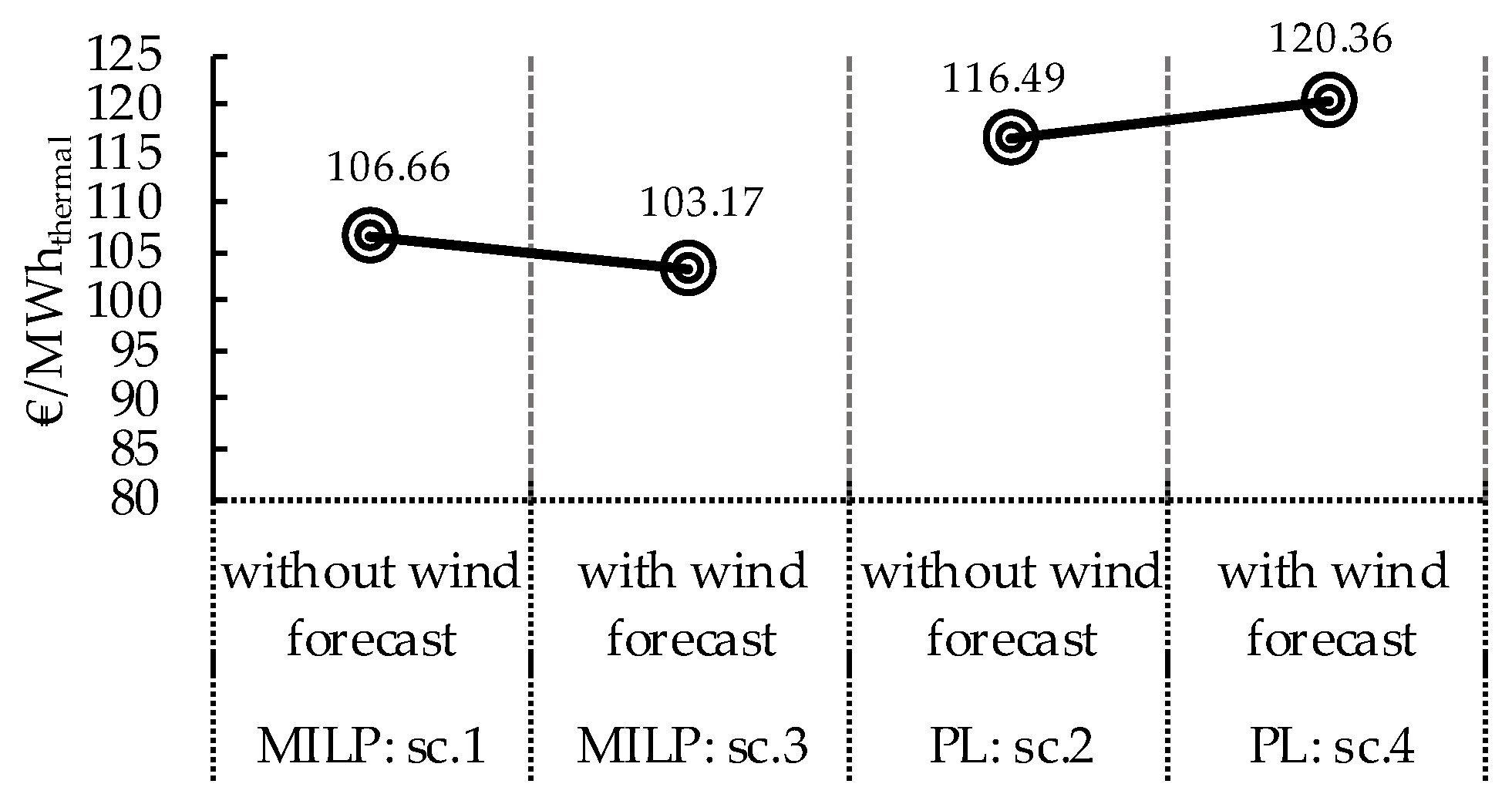
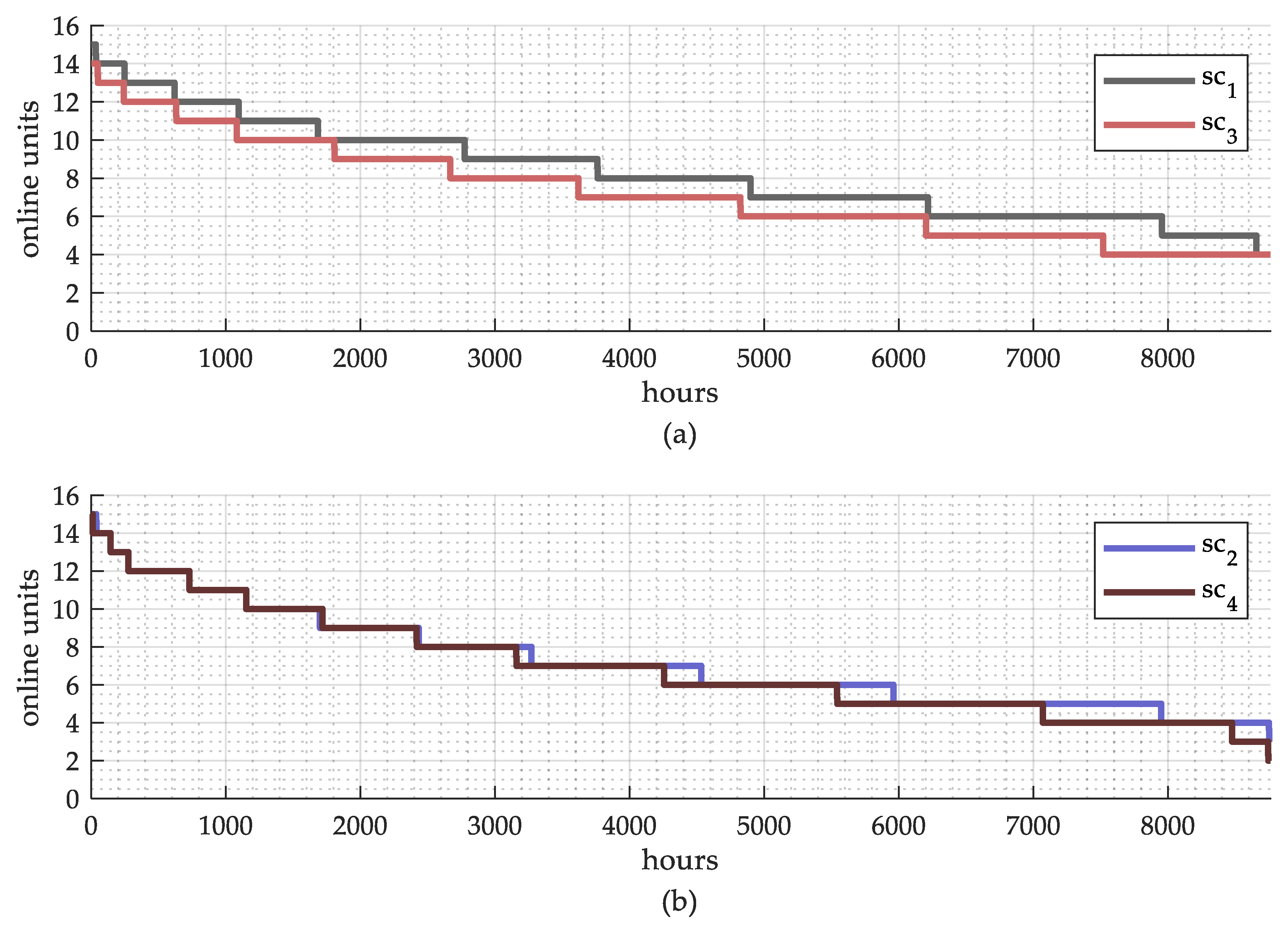
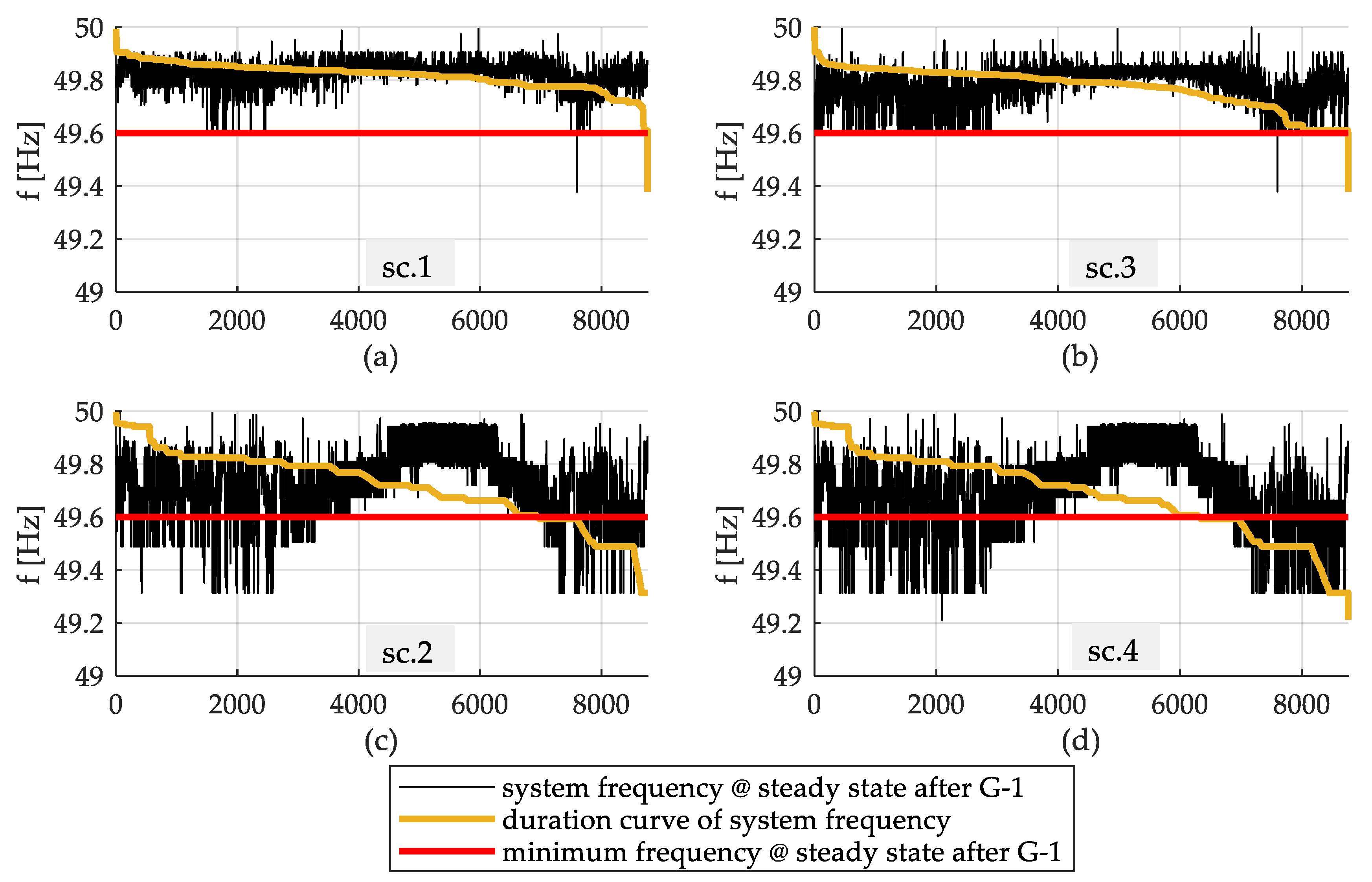
4.1.2. Annual Results

To obtain a more objective basis of comparison, the performance of the PL-UC and MILP-UC models is analyzed for the medium-sized island via annual simulations, taking also account of the effect that wind power forecasting may have on system operation. When a sophisticated UC-ED method is applied, it makes sense to assume that advanced wind prognosis capabilities will also be available in the ECC of the NII system. With simple PL-UC, wind power forecasting may not be available or it may rely on less sophisticated, even empirical, means. Nevertheless, to provide an equal basis for the comparison of the two methods, not biased by wind prognosis sophistication, two additional scenarios are examined involving perfect wind power forecasting. The new scenarios complement Scenarios 1 and 2, introduced in the previous section, to provide the envelope of wind prognosis capabilities:
  • Scenario 3: MILP-UC with perfect wind forecasting
  • Scenario 4: PL-UC with perfect wind forecasting
As observed in Figure 12 and Figure 13, the introduction of wind forecasting always increases wind penetration by 5–6%, greatly reducing wind curtailments, from almost 50% of primarily available wind energy down to 16%. The performance of the two methods is similar, with PL-UC achieving higher penetration in the absence of wind forecasting.
The variable generation cost of thermal units is expectedly lower when optimal management is applied via the MILP-UC method with a substantial reduction of 10-15% compared to the PL-UC method. With MILP-UC, the introduction of wind prognosis benefits generation cost by ~3.5 €/MWhthermal, confirming the significance of wind forecasting for the efficient management of isolated island systems. However, with the simplified PL-UC, the variable cost of conventional units increases by ~4 €/MWhthermal when forecasting is introduced (Figure 13), due to the more frequent commitment of expensive but flexible LFO units. The low ML levels and increased spinning reserves of these units lead to additional room for accommodating anticipated wind power when wind forecasting is applied.
System security is also severely impacted when the PL-UC method is applied. In Figure 14, the anticipated system frequency deviation is shown (cf. Figure 4) following loss of the largest online thermal unit, calculated according to Equation (32) [52]:
f t = f 0 ( 1 ( max u ( P u . t ) / u max u ( P u . t ) ( 1 / S u ) ) )
Assuming a permissible Δfss of 1.25% (or 0.675 Hz, for a 50 Hz system frequency), used also to quantify the primary active power reserves capability of the units, with the MILP-UC approach no violation of Δfss is observed throughout the year in Figure 14a,b, indicating that the method effectively maintains the prescribed security of operation requirements. It is worth noting that frequency deviations on average reach lower levels in Figure 14b, as fewer thermal units are committed in the presence of wind forecasting.
When the PL-UC method is applied (Figure 14c,d), the set frequency limit will potentially be violated over a large part of the year (11% increasing to 19% with wind forecasting) with an anticipated minimum below 49 Hz. Therefore, it is clear that the system is exposed to increased risks, while major disturbances will induce under-frequency load shedding.

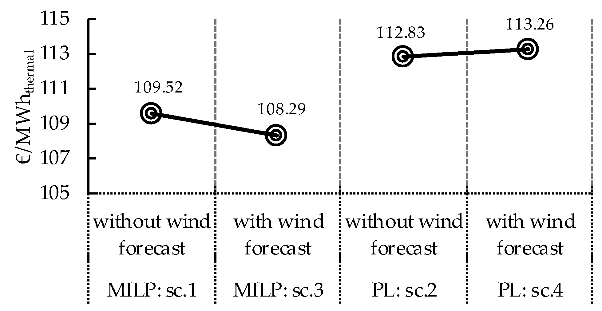
4.2. Annual Operation of Large-Size Island System

In this section, the annual operation of the large island system is investigated for the same scenarios as in the previous section.
In this case, the introduction of wind forecasting in the MILP-UC increases wind penetration only by ~1% point, with a reduction of wind curtailments, and an improvement of ~1 €/MWhthermal in system cost (Figure 15 and Figure 16). With the PL-UC method, wind forecasting achieves even less impressive results, as wind penetration increases by only 0.5% points, while wind curtailments and system cost also change little as well (Figure 15 and Figure 16).
The minor improvement achieved by wind forecasting in the case of the large island system, for both UC models, are mainly attributed to the technical characteristics of the thermal generation fleet (Table A3 and Table A4 of the Appendix A). The low ML levels of the units create enough room to absorb all available RES production, whether the UC pattern is derived employing wind forecasting or not. This indicates that the large NII system is effectively not saturated in terms of installed RES capacity.
Overall, the MILP-UC proves again superior in terms of generation cost, achieving a variable cost reduced by ~4–5 €/MWhthermal compared to the PL-UC (Figure 16). On the other hand, the PL-UC leads to a slightly higher wind penetration and reduced curtailments. This is attributed to the reduced number of committed units (Figure 17), as well as to the fact that the dynamic limitation (Equation (5)) does not account for primary reserves, leading to systematic overestimation of the wind absorption capability of the system (Figure 18). This, in turn, results in the relaxation of the dynamic limitation, with the minimum loading limitation now prevailing to determine the wind hosting capacity of the large NII system (Table 2).
Regarding system security, a permissible Δfss of 0.8% (or 0.4 Hz) is assumed in this case. Figure 19a,b shows that potential Δfss violations are effectively eliminated with the MILP-UC variant, while security of operation is systematically compromised with the PL-UC method (minimum permissible frequency level violated over 1810 to 2449 h per year, Figure 19c,d).

5. Conclusions

In this paper two alternative approaches to the unit commitment problem in NII systems are presented and comparatively assessed. The first model is based on priority listing, resembling the established simple generation scheduling practices in islands without ECC facilities. The second UC variant is based on a MILP optimization approach to determine generation scheduling, incorporating more sophisticated constraints and intended to be implemented within ECCs suitable for medium and large island systems.
Two NII power systems were considered as study cases, to evaluate the performance of the examined UC methods. Based on the annual results obtained by the unit commitment methods, the MILP-based UC proves to be superior in terms of generation cost and security of operation. PL-UC expectedly leads to a higher production cost and, most important, compromises system security, failing to recognize and maintain anticipated frequency excursions in case of major disturbances within applicable limits.
On the other hand, PL-UC is capable of creating more room to host available wind energy, especially in the absence of wind forecasting, by committing a reduced capacity of thermal units to fulfill the imposed spinning reserve criteria, albeit with a negative impact on system security, as well as at increased system operating cost, particularly in the case of the medium-size island. However, similar wind penetration levels are also possible with the MILP-UC, if RES absorption is further prioritized in its objective function, at the expense of higher production cost, as discussed in Reference [29].
Overall, although the PL-UC method is inferior to the MILP approach, it could still be a valid alternative for generation scheduling in islands without an advanced ECC infrastructure, leading to acceptable costs and good RES penetration rates, subject to the reservation of an inherently oversimplified quantification of system security constraints.

Author Contributions

The paper was a collaborative effort among the authors. The authors contributed collectively to the theoretical analysis, modeling, simulation, and manuscript preparation.

Funding

The work of Georgios N. Psarros is financially supported by the Alexander S. Onassis Public Benefit Foundation.

Acknowledgments

This work was partially supported by the Alexander S. Onassis Public Benefit Foundation.

Conflicts of Interest

The authors declare no conflicts of interest.

Nomenclature

Indices
tTime interval (period) of the optimization horizon
uConventional unit
eIndex of reserve types {pr, sr, tr}, for primary, secondary and tertiary reserves
bIndex of blocks of the linearized cost function of each thermal unit
Continuous Variables
C p Total production cost of all operating units
C s u Total start-up cost over the dispatch horizon
C s d Total shut-down cost over the dispatch horizon
C s l Total cost of slack variables
P u , t Production level of unit u
P w , t D 
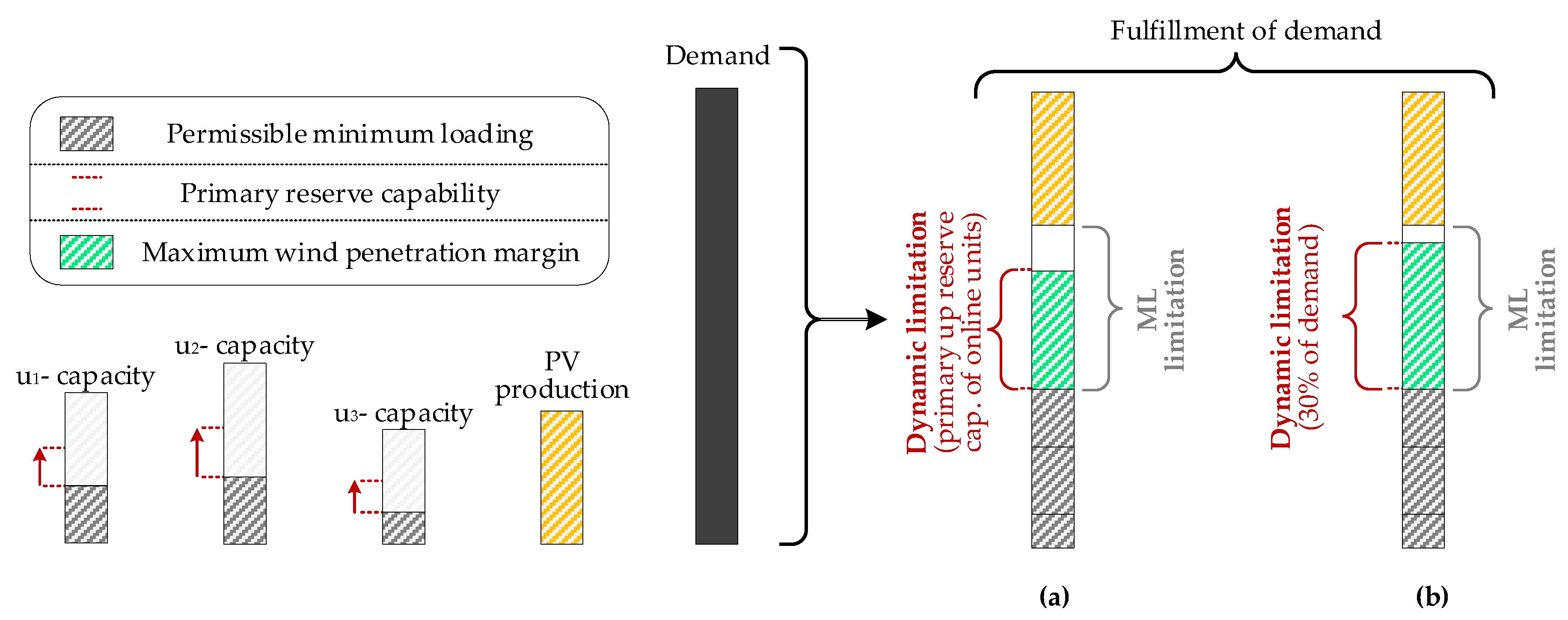
Dynamic limitation of wind power for period t
P w , t M L Minimum loading limitation of wind power for period t
r u , t , e u p / d n Type e reserve (up/down) provided by unit u in period t
r r t , e u p / d n Type e reserve requirements (up/down) in period t
x , t Slack variable for quantity *
Δ P u , t , b Production level of unit u at block b in dispatch period t
Binary Variables
s u u , t Binary variable equal to 1 if unit u starts up at t
s d u , t Binary variable equal to 1 if unit u shuts down at t
s t u , t Binary variable equal to 1 if unit u is online at t
v u , b Binary variable equal to 1 if the power output of unit u at t exceeds block b
Parameters
C u min Variable operating cost of unit u at minimum loading level
C u S U Start-up cost of unit u per start-up event
C u S D Shut-down cost of unit u per shut-down event
f 0 System frequency before disturbance
f t System frequency after the disturbance (loss of largest unit)
P L , t Total demand in period t
P u max Maximum power output of unit u in period t
P u min Minimum power output of unit u in period t
P w , t Total wind production in period t
P w , t e Estimated wind production in period t
P w , t a Actual wind production in period t
R u , e Type e reserves capability of unit u
r d u Ramp down rate of unit u
r u u Ramp up rate of unit u
S u Droop characteristic of unit u
T u , b g Upper limit of block b of the variable cost of unit u
c D Dynamic limitation coefficient for wind penetration in PL-UC
l w Coefficient quantifying the proportion of wind power that may be suddenly lost
Δ f s s Permissible frequency drop at steady state conditions, after a severe disturbance
ε Coefficient expressing the level of load-related spinning reserves in PL-UC
κ * Penalty factor for the relaxation of constraints for quantity x , t in MILP-UC
λ u , b Slope of block b of the variable cost of unit u

Appendix A

The assumed technical and economic parameters of conventional units are presented in Table A1, Table A2, Table A3 and Table A4 for the study-case medium and large island systems. More detailed characteristics for the large NII power system can be found in Reference [7]. Unit u1 of Table A3 and Table A4 is considered “must run”, i.e., maintained online throughout the year.
For the medium-sized island, a permissible frequency drop at steady state conditions after a severe disturbance (Δfss) of 1.25% is assumed, leading to primary reserves capability of the units equal to 25% of their rated capacity. For the large system this limit is set to 0.8%, resulting in 16% and 20% primary reserves capabilities for a 5% and 4% droop respectively.
Table A1. Technical characteristics of conventional units of the medium-sized study-case system.
UnitPrioritySeasonal UsagePmaxPminrurdS (%)
(MW)(MW/min)
1–31–312.07.00.600.605%
4,54,58.04.00.400.405%
667.54.50.280.285%
775.03.00.250.255%
887.52.00.750.755%
9915.03.01.301.305%
10–1410–143.01.00.150.155%
Table A2. Economic characteristics of conventional units of the medium-sized study-case system.
UnitFuelOperating Point (% of Pmax)Fuel Consumption @ Operating Point (kg/kWh)
ABCABC
1–3HFO63%83%100%0.2110.1980.206
4–5HFO50%75%100%0.2200.2080.225
6HFO67%80%93%0.2350.2150.220
7HFO64%80%90%0.2050.1950.201
8LFO33%67%87%0.3600.2900.315
9LFO31%65%100%0.4000.3800.410
10–14LFO50%73%93%0.2650.2600.262
Table A3. Technical characteristics of conventional units of the large-sized study-case system.
Unit PrioritySeasonal UsagePmaxPminrurdS (%)
(MW)(MW/min)
1,21,215.010.00.750.755%
3–615–1825.04.51.251.255%
7–813,1412.05.00.600.605%
9–1110–1223.014.01.151.155%
12–183–917.06.50.850.854%
Table A4. Economic characteristics of conventional units of the large-sized study-case system.
Unit FuelOperating Point (% of Pmax)Fuel Consumption @ Operating Point (kg/kWh)
ABCABC
1,2HFO70%85%100%0.3100.3080.320
3–6LFO30%65%100%0.4000.3500.360
7,8HFO50%75%100%0.2100.2050.204
9–11HFO75%90%100%0.2150.2130.214
12–18HFO45%75%100%0.2250.2150.216

References

  1. Erdinc, O.; Paterakis, N.G.; Catalão, J.P.S. Overview of insular power systems under increasing penetration of renewable energy sources: Opportunities and challenges. Renew. Sustain. Energy Rev. 2015, 52, 333–346. [Google Scholar] [CrossRef] [Green Version]
  2. Hatziargyriou, N.; Margaris, I.; Stavropoulou, I.; Papathanassiou, S.; Dimeas, A. Noninterconnected Island Systems: The Greek Case. IEEE Electrif. Mag. 2017, 5, 17–27. [Google Scholar] [CrossRef]
  3. Egido, I.; Fernandez-Bernal, F.; Centeno, P.; Rouco, L. Maximum frequency deviation calculation in small isolated power systems. IEEE Trans. Power Syst. 2009, 24, 1731–1738. [Google Scholar] [CrossRef]
  4. Delille, G.; François, B.; Malarange, G. Dynamic Frequency Control Support by Energy Storage to Reduce the Impact of Wind and Solar Generation on Isolated Power System’s Inertia. IEEE Trans. Sustain. Energy 2012, 3, 931–939. [Google Scholar] [CrossRef]
  5. Papathanassiou, S.A.; Boulaxis, N.G. Power limitations and energy yield evaluation for wind farms operating in island systems. Renew. Energy 2006, 31, 457–479. [Google Scholar] [CrossRef]
  6. Karamanou, E.; Papathanassiou, S.; Boulaxis, N. Operating policies for autonomous Island grids with PV penetration. In Proceedings of the 4th European PV-Hybrid and Mini-Grid Conference, Athens, Greece, 29–30 May 2008. [Google Scholar]
  7. Psarros, G.N.; Karamanou, E.G.; Papathanassiou, S.A. Feasibility Analysis of Centralized Storage Facilities in Isolated Grids. IEEE Trans. Sustain. Energy 2018, 9, 1822–1832. [Google Scholar] [CrossRef]
  8. Psarros, G.N.; Kokkolios, S.P.; Papathanassiou, S.A. Centrally Managed Storage Facilities in Small Non-Interconnected Island Systems. In Proceedings of the 2018 53rd International Universities Power Engineering Conference (UPEC), Glasgow, UK, 4–7 September 2018. [Google Scholar]
  9. Brown, P.D.; Pecas Lopes, J.A.; Matos, M.A. Optimization of Pumped Storage Capacity in an Isolated Power System With Large Renewable Penetration. IEEE Trans. Power Syst. 2008, 23, 523–531. [Google Scholar] [CrossRef] [Green Version]
  10. Vasconcelos, H.; Moreira, C.; Madureira, A.; Lopes, J.P.; Miranda, V. Advanced Control Solutions for Operating Isolated Power Systems: Examining the Portuguese islands. IEEE Electrif. Mag. 2015, 3, 25–35. [Google Scholar] [CrossRef]
  11. Bakirtzis, A.G.; Dokopoulos, P.S. Short term generation scheduling in a small autonomous system with unconventional energy sources. IEEE Trans. Power Syst. 1988, 3, 1230–1236. [Google Scholar] [CrossRef]
  12. Contaxis, G.C.; Kabouris, J. Short term scheduling in a wind/diesel autonomous energy system. IEEE Trans. Power Syst. 1991, 6, 1161–1167. [Google Scholar] [CrossRef]
  13. Papaefthymiou, S.V.; Karamanou, E.G.; Papathanassiou, S.A.; Papadopoulos, M.P. A wind-hydro-pumped storage station leading to high RES penetration in the autonomous island system of Ikaria. IEEE Trans. Sustain. Energy 2010, 1, 163–172. [Google Scholar] [CrossRef]
  14. Lujano-Rojas, J.M.; Osório, G.J.; Catalão, J.P.S. New probabilistic method for solving economic dispatch and unit commitment problems incorporating uncertainty due to renewable energy integration. Int. J. Electr. Power Energy Syst. 2016, 78, 61–71. [Google Scholar] [CrossRef]
  15. Kazemi, M.; Siano, P.; Sarno, D.; Goudarzi, A. Evaluating the impact of sub-hourly unit commitment method on spinning reserve in presence of intermittent generators. Energy 2016, 113, 338–354. [Google Scholar] [CrossRef]
  16. Papathanassiou, S.; Papalexopoulos, A.D.; Andrianesis, P. Energy Control Centers and Electricity Markets in the Greek Non-Interconnected Islands. In Proceedings of the MedPower 2014, Athens, Greece, 2–5 November 2014; p. 46. [Google Scholar]
  17. Catalão, J.P.S. Electric Power Systems: Advanced Forecasting Techniques and Optimal Generation Scheduling; CRC Press: Boca Raton, FL, USA, 2012; ISBN 978-1-4398-9396-8. [Google Scholar]
  18. Frangioni, A.; Gentile, C.; Lacalandra, F. Tighter Approximated MILP Formulations for Unit Commitment Problems. IEEE Trans. Power Syst. 2009, 24, 105–113. [Google Scholar] [CrossRef] [Green Version]
  19. Padhy, N.P. Unit Commitment—A Bibliographical Survey. IEEE Trans. Power Syst. 2004, 19, 1196–1205. [Google Scholar] [CrossRef]
  20. Morales-Espana, G.; Latorre, J.M.; Ramos, A. Tight and Compact MILP Formulation for the Thermal Unit Commitment Problem. IEEE Trans. Power Syst. 2013, 28, 4897–4908. [Google Scholar] [CrossRef]
  21. Morales-Espana, G.; Latorre, J.M.; Ramos, A. Tight and Compact MILP Formulation of Start-Up and Shut-Down Ramping in Unit Commitment. IEEE Trans. Power Syst. 2013, 28, 1288–1296. [Google Scholar] [CrossRef]
  22. Simoglou, C.K.; Kardakos, E.G.; Bakirtzis, E.A.; Chatzigiannis, D.I.; Vagropoulos, S.I.; Ntomaris, A.V.; Biskas, P.N.; Gigantidou, A.; Thalassinakis, E.J.; Bakirtzis, A.G.; et al. An advanced model for the efficient and reliable short-term operation of insular electricity networks with high renewable energy sources penetration. Renew. Sustain. Energy Rev. 2014, 38, 415–427. [Google Scholar] [CrossRef]
  23. Chang, G.W.; Chuang, C.S.; Lu, T.K.; Wu, C.C. Frequency-regulating reserve constrained unit commitment for an isolated power system. IEEE Trans. Power Syst. 2013, 28, 578–586. [Google Scholar] [CrossRef]
  24. Sokoler, L.E.; Vinter, P.; Baerentsen, R.; Edlund, K.; Jorgensen, J.B. Contingency-Constrained Unit Commitment in Meshed Isolated Power Systems. IEEE Trans. Power Syst. 2016, 31, 3516–3526. [Google Scholar] [CrossRef]
  25. Simoglou, C.K.; Bakirtzis, E.A.; Biskas, P.N.; Bakirtzis, A.G. Optimal operation of insular electricity grids under high RES penetration. Renew. Energy 2016, 86, 1308–1316. [Google Scholar] [CrossRef]
  26. Asensio, M.; Contreras, J. Stochastic Unit Commitment in Isolated Systems With Renewable Penetration Under CVaR Assessment. IEEE Trans. Smart Grid 2016, 7, 1356–1367. [Google Scholar] [CrossRef]
  27. Ntomaris, A.V.; Bakirtzis, E.A.; Chatzigiannis, D.I.; Simoglou, C.K.; Biskas, P.N.; Bakirtzis, A.G. Reserve Quantification in Insular Power Systems with High Wind Penetration. In Proceedings of the IEEE PES Innovative Smart Grid Technologies, Europe, Istanbul, Turkey, 12–15 October 2014; pp. 1–6. [Google Scholar]
  28. Tian, Y.; Fan, L.; Tang, Y.; Wang, K.; Li, G.; Wang, H. A Coordinated Multi-Time Scale Robust Scheduling Framework for Isolated Power System With ESU Under High RES Penetration. IEEE Access 2018, 6, 9774–9784. [Google Scholar] [CrossRef]
  29. Psarros, G.N.; Nanou, S.I.; Papaefthymiou, S.V.; Papathanassiou, S.A. Generation scheduling in non-interconnected islands with high RES penetration. Renew. Energy 2018, 115, 338–352. [Google Scholar] [CrossRef]
  30. Psarros, G.N.; Papathanassiou, S.A. Bi-level Minimum Loading Unit Commitment for Small Isolated Power Systems. In Proceedings of the MedPower 2018, Dubrovnik, Croatia, 12–15 November 2018. [Google Scholar]
  31. Psarros, G.N.; Papathanassiou, S.A. Comparative Assessment of Unit Commitment Methods for Isolated Island Grids. In Proceedings of the 2018 53rd International Universities Power Engineering Conference (UPEC), Glasgow, UK, 4–7 September 2018. [Google Scholar]
  32. Caralis, G.; Christakopoulos, T.; Karellas, S.; Gao, Z. Analysis of energy storage systems to exploit wind energy curtailment in Crete. Renew. Sustain. Energy Rev. 2019, 103, 122–139. [Google Scholar] [CrossRef]
  33. Kundur, P.; Paserba, J.; Ajjarapu, V.; Andersson, G.; Bose, A.; Van Cutsem, T.; Canizares, C.; Hatziargyriou, N.; Hill, D.; Vittal, V.; et al. Definition and Classification of Power System Stability IEEE/CIGRE Joint Task Force on Stability Terms and Definitions. IEEE Trans. Power Syst. 2004, 19, 1387–1401. [Google Scholar] [CrossRef]
  34. Arroyo, J.M.; Conejo, A.J. Optimal response of a thermal unit to an electricity spot market. IEEE Trans. Power Syst. 2000, 15, 1098–1104. [Google Scholar] [CrossRef]
  35. Carrion, M.; Arroyo, J.M. A Computationally Efficient Mixed-Integer Linear Formulation for the Thermal Unit Commitment Problem. IEEE Trans. Power Syst. 2006, 21, 1371–1378. [Google Scholar] [CrossRef]
  36. Wood, A.; Wollenberg, B.; Shebleeacute, G. Power Generation, Operation and Control, 3rd ed.; Wiley: Hoboken, NJ, USA, 2013; ISBN 9780471790556. [Google Scholar]
  37. Shahidehpour, M.; Yamin, H.; Li, Z. Market Operations in Electric Power Systems: Forecasting, Scheduling, and Risk Management; Wiley: Hoboken, NJ, USA, 2009; ISBN 9781424442416. [Google Scholar]
  38. General Algebraic Modeling System (GAMS). Available online: https://www.gams.com/ (accessed on 19 December 2016).
  39. IBM CPLEX Optimizer. Available online: https://www-01.ibm.com/software/commerce/optimization/cplex-optimizer/ (accessed on 19 December 2016).
  40. Thomas, D.; Deblecker, O.; Ioakimidis, C.S. Optimal design and techno-economic analysis of an autonomous small isolated microgrid aiming at high RES penetration. Energy 2016, 116, 364–379. [Google Scholar] [CrossRef]
  41. Miranda, I.; Silva, N.; Leite, H. A Holistic Approach to the Integration of Battery Energy Storage Systems in Island Electric Grids with High Wind Penetration. IEEE Trans. Sustain. Energy 2016, 7, 775–785. [Google Scholar] [CrossRef]
  42. Kuo, M.; Lu, S.-D.; Tsou, M.-C. Considering Carbon Emissions in Economic Dispatch Planning for Isolated Power Systems: A Case Study of the Taiwan Power System. IEEE Trans. Ind. Appl. 2018, 54, 987–997. [Google Scholar] [CrossRef]
  43. Solanki, B.V.; Bhattacharya, K.; Canizares, C.A. A Sustainable Energy Management System for Isolated Microgrids. IEEE Trans. Sustain. Energy 2017, 8, 1507–1517. [Google Scholar] [CrossRef]
  44. Andersson, G. Dynamics and Control of Electric Power Systems; EEH-Power Systems Laboratory ETH: Zurich, Switzerland, 2012. [Google Scholar]
  45. Lee, Y.; Baldick, R. A Frequency-Constrained Stochastic Economic Dispatch Model. IEEE Trans. Power Syst. 2013, 28, 2301–2312. [Google Scholar] [CrossRef]
  46. Ahmadi, H.; Ghasemi, H. Security-constrained unit commitment with linearized system frequency limit constraints. IEEE Trans. Power Syst. 2014, 29, 1536–1545. [Google Scholar] [CrossRef]
  47. Wen, Y.; Li, W.; Huang, G.; Liu, X. Frequency Dynamics Constrained Unit Commitment With Battery Energy Storage. IEEE Trans. Power Syst. 2016, 31, 5115–5125. [Google Scholar] [CrossRef]
  48. Hansen, C.W.; Papalexopoulos, A.D. Operational Impact and Cost Analysis of Increasing Wind Generation in the Island of Crete. IEEE Syst. J. 2012, 6, 287–295. [Google Scholar] [CrossRef]
  49. Dokopoulos, P.S.; Saramourtsis, A.C.; Bakirtzis, A.G. Prediction and evaluation of the performance of wind-diesel energy systems. IEEE Trans. Energy Convers. 1996, 11, 385–393. [Google Scholar] [CrossRef]
  50. Andrianesis, P.; Liberopoulos, G.; Varnavas, C. The impact of wind generation on isolated power systems: The case of Cyprus. In Proceedings of the 2013 IEEE Grenoble Conference, Grenoble, France, 16–20 June 2013; pp. 1–6. [Google Scholar]
  51. Papalexopoulos, A.; Vitellas, I.; Hatziargyriou, N.D.; Hansen, C.; Patsaka, T.; Dimeas, A.L. Assessment and economic analysis of wind generation on the ancillary services and the unit commitment process for an isolated system. In Proceedings of the 2011 16th International Conference on Intelligent System Applications to Power Systems, Hersonissos, Greece, 25–28 September 2011; pp. 1–6. [Google Scholar]
  52. Kundur, P. Power System Stability and Control, 1st ed.; McGraw-Hill Education: New York, NY, USA, 1994; ISBN 978-0070359581. [Google Scholar]
Figure 1. Logical process for simulating the PL-UC.
Energies 12 00657 g001
Figure 2. (a) Actual variable operating cost curve of a thermal unit in grey line; (b) piecewise linearization of cost curve to be implemented in the MILP-UC.
Energies 12 00657 g002
Figure 3. (a) Spinning and (b) primary up reserves capabilities of the online units u1 and u2.
Energies 12 00657 g003
Figure 4. (a) System frequency response, (b) power output of a single thermal unit, and (c) speed droop characteristic of the unit.
Energies 12 00657 g004
Figure 5. Illustrative representation of wind absorption margin employing the minimum loading and dynamic limitations, employing (a) the MILP-UC and (b) the PL-UC method.
Energies 12 00657 g005
Figure 6. Participation of each thermal unit in meeting system demand when (a) PL-UC and (b) MILP-UC is applied.
Energies 12 00657 g006
Figure 7. Spinning and primary up reserves surplus/deficit when the PL-UC variant is applied for an indicative low-demand day. Positive/negative values denote surplus/deficit.
Energies 12 00657 g007
Figure 8. Number of committed units per time interval, for the PL- and MILP-UC models.
Energies 12 00657 g008
Figure 9. Maximum wind penetration margin per time interval, for the PL and MILP UC model formulations.
Energies 12 00657 g009
Figure 10. Minimum loading and dynamic limitation for the examined day, assuming lw = 50%. (a) PL-UC based on (4), (5) and (b) MILP-UC based on (28), (29).
Energies 12 00657 g010
Figure 11. Variable cost of thermal units in €/MWh, per time interval, for the PL- and MILP-UC model Figure 4.
Energies 12 00657 g011
Figure 12. Medium-sized NII system. (a) Annual wind penetration levels in % of total demand, and (b) Wind curtailments in % of available wind energy, per examined scenario.
Energies 12 00657 g012
Figure 13. Medium-sized NII system. Variable cost of thermal units in €/MWhthermal, per examined scenario.
Energies 12 00657 g013
Figure 14. Medium-size NII system. Anticipated frequency deviations should a severe disturbance take place (loss of largest online unit), as calculated by Equation (32), with (a), (b) the MILP and (c), (d) the PL-UC approach (Scenarios 1, 3 and 2, 4 respectively).
Energies 12 00657 g014
Figure 15. Large-sized NII system. (a) Annual wind penetration levels in % of total demand, and (b) Wind curtailments in % of available wind energy, per examined scenario.
Energies 12 00657 g015
Figure 16. Large-sized NII system. Variable cost of thermal units in €/MWhthermal, per examined scenario.
Energies 12 00657 g016
Figure 17. Large-sized NII system. (a) Duration curve of online unit number for Scenarios 1 and 3 (MILP-UC); (b) Duration curve of online units for Scenarios 2 and 4 (PL-UC).
Energies 12 00657 g017
Figure 18. Large-sized NII system. Duration curve of dynamic limitation estimation differences by Equations (5) and (29). Positive values denote overestimation by PL-UC compared to MILP-UC.
Energies 12 00657 g018
Figure 19. Large-sized NII system. Anticipated frequency deviations should a severe disturbance take place (loss of largest online unit), as calculated by Equation (32), with (a), (b) the MILP and (c), (d) the PL-UC approach (Scenarios 1, 3 and 2, 4 respectively).
Energies 12 00657 g019
Table 1. PL-UC vs MILP-UC during a low-demand day, for the medium-sized island.
h/uu1u2u3u4u5u6u7u8u9Net Load (MW)
1○ ●○ -○ ●○ ●- ●- -- ●- -- -31
2○ ●○ -○ ●○ ●- ●- -- ●- -- -28
3○ ●○ -○ ●○ ●- ●- -- ●- -- -26
4○ ●○ -○ ●- ●- ●- -- -- -- -23
5○ ●○ -○ ●- ●- ●- -- -- -- -23
6○ ●○ -○ ●- ●- ●- -- -- -- -23
7○ ●○ -○ ●- ●- ●- -- -- -- -23
8○ ●○ -○ ●○ ●- ●- -- ●- -- -28
9○ ●○ ●○ ●○ ●- ●- -- -○ -- -34
10○ ●○ ●○ ●○ ●- ●- -- -○ -- -36
11○ ●○ ●○ ●○ ●○ ●- -- ●- -- -40
12○ ●○ ●○ ●○ ●- ●- -- ●- -○ -41
13○ ●○ ●○ ●○ ●○ ●- -- ●- -- -39
14○ ●○ ●○ ●○ ●○ ●- -- ●- -- -38
15○ ●○ ●○ ●○ ●○ ●- -- ●- -- -39
16○ ●○ ●○ ●○ ●○ ●- -- ●- -- -35
17○ ●○ ●○ ●○ -- ●- -- ●- -- -31
18○ ●○ ●○ ●○ -- ●- -- ●- -- -32
19○ ●○ ●○ ●○ -- ●- -- ●○ -- -36
20○ ●○ ●○ ●○ -- ●- -- ●○ -- -36
21○ ●○ ●○ ●○ ●○ ●- -- ●○ -- -42
22○ ●○ ●○ ●○ ●○ ●- ●- ●- -○ -50
23○ ●○ ●○ ●○ ●○ ●- ●- -○ -- -45
24○ ●○ ●○ ●○ ●○ ●- -- -- -- -38
○ PL-UC with G-1 criterion; ● MILP-UC; - not committed.
Table 2. Prevalent limitation (dynamic or technical minimum) for determining the wind hosting capacity of the large NII system, per examined scenario.
Scenario1234
UC variantMILPPLMILPPL
Minimum loading limitation (h)7914876040828760
Dynamic limitation (h)846046780

