Performance Comparison of Mismatch Power Loss Minimization Techniques in Series-Parallel PV Array Configurations

Abstract

The mismatch in current-voltage (I-V) characteristics of photovoltaic (PV) modules causes significant power loss in a large PV array, which is known as mismatch power loss (MML). The PV array output power generation can be improved by minimizing MML using different techniques. This paper investigates the performance of different module arrangement techniques to minimize MML both for long series string (LSS) and long parallel branch (LPB) in series-parallel (SP) array configurations at uniform irradiance condition. To investigate the significance of MML LSS-SP configuration with dimensions: 1 × 40, 2 × 20, 4 × 10, 5 × 8 and LPB-SP configuration with dimensions: 40 × 1, 20 × 2, 10 × 4, 8 × 5 were used. A comparative analysis is made to find the effectiveness of MML reduction techniques on PV arrays with three different power ratings. Simulation results show that the PV modules arrangement obtained by the genetic algorithm (GA) and current based arrangement (Im) performed better than the arrangements obtained by all other techniques in terms of PV array output power and MML minimization. The performance of the proposed technique was analyzed for both LSS-SP and LPB-SP array configurations in 400 W, 3400 W, and 9880 W arrays. To substantiate the simulation results experiment was performed using a 400 W PV array in outdoor weather condition and obtained similar results. It was also observed that the percentage of recoverable energy (%RE) obtained by arranging the modules using the GA method was higher than Im based method for both LSS-SP and LPB-SP array configurations. A maximum %RE of 4.159 % was recorded for a 5 × 8 LSS-SP array configuration by applying the GA based MML reduction method.

1. Introduction

The utilization of solar energy has received remarkable attention across the globe over the last decade [1]. Researchers are constantly working to find the means and ways for further improving the performance of the existing technologies and developing more efficient methods of utilization of solar energy. Currently, PV technology is one of the widely used renewable energy technologies that is being motivated by the global scenario of increasing energy demand. In many applications, such as hybrid solar power plants [2], building-integrated photovoltaic (BIPV) systems [3,4,5], solar-powered vehicle battery charging systems [6], grid-connected PV systems [7,8,9], solar powered water pumping systems [10], micro-grid PV systems [11], solar PV arrays are used in different dimensions and configurations according to the system requirements. There are various configurations possible to arrange PV modules in an array such as SP, total cross tied (TCT), bridge-linked (BL) [12], and honey-comb (HC), but most practically used configuration is SP.

The MML of a PV array modules depends on several factors such as the availability of solar radiation and its spectral distribution, PV module operating temperature (causes 9% power loss due to a 20-degree temperature differences between hot and cold modules), shading, uneven soiling (causes 1% to 4% power loss) PV modules manufacturing tolerance (causes 4% to 7% power loss in a new array), and PV power degradation (averagely 0.7% per year) [13] by aging [14,15]. Among them, MML due to manufacturing tolerance is one of the significant factors. MML is caused by the I-V characteristics mismatch of PV modules, which is a common phenomenon in a PV array [16].

Besides, the shape of the I-V curve of a PV module depends on the series and shunt resistances [17,18]. The effect of series resistance, Rs and shunt resistance, Rp on the I-V curve, is explained elaborately in References [19,20] with graphical representation both for two diode model and simplified one diode model. In Reference [21], a novel simplified two diode model of PV module is developed by neglecting the Rs and Rp in order to reduce computational time with accurate output response during temperature and radiation changes. Therefore, the simplified PV model can be useful for design a PV array and also for MML analysis.

In an array, the output power is undoubtedly less than the summation of individual module’s power because new PV modules with the same power rating and even from the same manufacturer are not precisely identical due to manufacturing tolerances. In PV modules manufacturing technology, manufacturing tolerances of ±3% to ±5% in their maximum power rating are generally allowed [22]. MML is recognized and investigated by many researchers on different size of PV array configurations using different reconfiguration techniques of PV modules [23,24,25].

To maximize the PV array output power, by minimizing MML, module sorting techniques had gained popularity among the researchers. To obtain minimum MML, photovoltaic maximum power parameters, such as max-power current, Im; short circuit current, Isc; max-power point power, Pm; max-power voltage, Vm; and open circuit voltage, Voc are typically used as PV module sorting parameters for the arrangement of newly installed PV array at uniform radiation condition. This approach is similar to cell sorting for modules to minimize the MML [26,27] during module manufacturing,

In the work in Reference [28], MML due to I-V mismatch in PV modules is first introduced, where the parameters Im and Vm are used to analyze both series and parallel PV string power losses at uniform radiation condition. In Reference [29], three max-power parameters Im, Vm and Pm are used as a module sorting variables for a 700 V, 400 kW PV array, where the result shows that Im based method reduces MML and produces more array power than Vm and Pm methods. In the work in Reference [30], MML is compared by arranging 40 PV modules between Im based arrangement with most commonly used random arrangement technique. Here, the result shows that minimum MML is obtained by Im based method. In above literature, it is clear that MML in PV array depends on modules sorting (arrangement) technique, hence, further investigation is required to find an optimal arrangement technique to achieve minimum MML in array output.

The GA based optimal arrangement technique was first adopted in Reference [31] for arranging new PV modules in an array to minimize MML at uniform irradiance condition. A simulation-based performance was investigated by using different LSS-SP array (3 × 6, 4 × 10, 5 × 13 and 5 × 18) configurations of 95 W modules and compared with conventional module arrangement techniques (Im, Isc, and Pm). In Reference [31], simulation results show that MML can be minimized less than 1% using GA technique whereas MML is always higher than 1.02% for other conventional module arrangement techniques by Im, Isc, and Pm.

In the work in Reference [32], a (9 × 9) TCT PV array reconfiguration is arranged using GA based technique under partial shading conditions to minimize MML. In Reference [33], the concept of standard deviation (SD) and GA based methods are applied in a (9 × 9) TCT PV array reconfiguration to minimize MML at partial shading condition. In Reference [34], a (3 × 2) SP PV array reconfiguration is compared between GA and Brute Force (BF) techniques during partial shading, where results show a very superior performance of GA for output power. In the work in Reference [35], an adaptive GA based reconfiguration technique is applied to a (4 × 4) SP PV array to maximize the output power of the PV array under the different pattern of partial shading conditions. In Reference [36], a GA based optimal reconfiguration technique is applied to a PV array to maximize the output power at partial shading condition. There are some other reconfiguration techniques are developed in References [25,37], to reduce MML due to partial shading.

The above literature review shows that PV modules arrangement technique using maximum power parameters is a prevalent practice to reduce MML in SP PV array configurations. Besides, GA also gained popularity as a PV array modules reconfiguration technique mostly at partial shading condition. To the author’s knowledge, to minimize the MML in a large PV generation at uniform irradiance condition the GA based module arrangement technique has only investigated on LSS-SP array configurations, not for LPB-SP array configurations. Furthermore, experimental validation for the latter has not been performed yet [31]. Therefore, applying and experimentally validating GA as a module arrangement technique is one of the main objectives of this work.

This paper presents simulation and experimental comparison of MML reduction in SP PV arrays using different techniques of module arrangement. The comparison has been made with the performance GA technique and other conventional techniques using 400 W, 3400 W, and 9880 W arrays each consists of 40 PV modules of 10 W, 85 W, and 247 W, respectively. The corresponding array output power and MML are calculated for both LSS-SP and LPB-SP arrays. For this work, 1 × 40, 2 × 20, 4 × 10 and 5 × 8 (parallel × series) array arrangements are used as LSS-SP array while 40 × 1, 20 × 2, 10 × 4 and 8 × 5 array arrangements are considered as LPB-SP array configurations. Finally, the experimental %RE is calculated and compared for 400 W (LSS-SP and LPB-SP) array configurations by applying GA based method and Im based method.

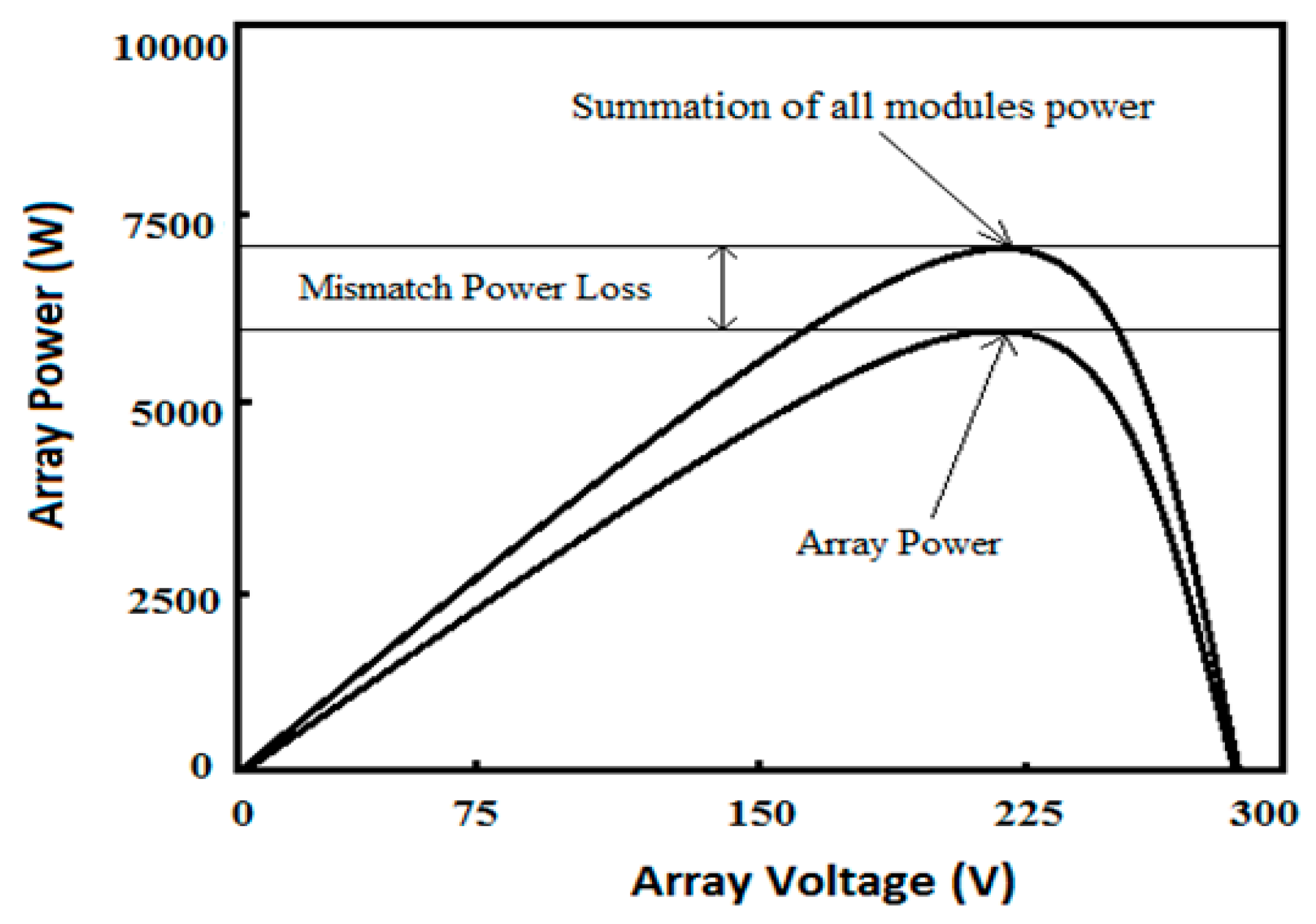
2. Mismatch Power Loss in PV Array

In a PV array, all modules do not have identical I-V characteristics even from the same manufacturer and same power ratings. I-V characteristic parameters are considered as Voc, Isc, Vm, Isc, and Pm. The I-V mismatch means differences of these I-V parameters between individual modules, which cause MML in a PV array. There are some constant factors such as manufacturer tolerance, light-induced power degradation, uneven surface soiling, discoloration, and cracking are responsible for I-V mismatch in new PV array modules; causes typically 4%–7% energy loss [38].

On the other hand, non-uniform irradiance or partial shading is considered as momentary factors of I-V mismatch in PV array modules [39,40,41]. It might occur by fallen leaves of trees, suddenly moving clouds over the photovoltaic array, the shadow of anything situated near the PV plant. All these factors are causes difference in modules I-V parameters, and this dissimilitude is the critical source of MML in PV array. Shading is a widespread issue for MML in PV array [42], and different novel algorithms and techniques have already been developed to reduce MML due to shading effects [43,44]. The manufacturing process of PV modules are developing competitively day by day to minimize the manufacturing variance of I-V parameters in same power rated modules, but still, now the available crystalline PV modules in the market contain manufacturing tolerances of ±3% to ±5% in their power rating. Due to this manufacturing tolerance level in case of high volume of PV modules in an array, the MML increases significantly. Hence, in this work MML are considered as coming from manufacturing tolerances.

Figure 1 shows that before connecting the modules in the array, the summation of individual modules power is higher than the array power and their corresponding power difference is defined as mismatch power. Therefore, to minimize MML due to manufacturing I-V mismatch in PV modules, this is essential to maximize the array power, by arranging array modules applying optimal configuration technique.

3. Mathematical Model of MML in SP Configuration

In SP array configurations, series connected modules work at the same amount of current in a string, and parallel strings work at the same amount of voltage at a time. As a rule, the Kirchhoff voltage law (KVL) is applied for string voltage calculation, and the Kirchhoff current law (KCL) is used for the array current calculation. Therefore, according to KVL, the string voltage equals the summation of modules voltage in the string, and according to KCL, the array current equals the summation of string current in the array [31]. However, in a practical PV array, a central maximum power point tracker (MPPT) [45,46,47,48] is used to get its global maximum power (GMPP) [49,50,51,52]. Therefore, all modules are led to work at their maximum potential, which is not exactly same for all modules even from same power rating due to the manufacturing tolerances, which causes MML in the PV array. For example, if two modules are connected in series having non-identical Im, then they compromise to operate at lower Im and similarly two parallel connected modules are having different Vm operate at lower Vm [31,53,54].

Now, consider a PV string be made up of X series-connected PV modules, with string voltage, $V_{String}^{mpp}$ and string current, $I_{String}^{mpp}$ The string voltage and current of the Pth PV module can be denoted by $V_{Module,P}^{mpp}$ and $I_{Module,P}^{mpp}$ respectively. With this notation, maximum string voltage and current can be expressed as follows.

$$V_{String}^{mpp}={\displaystyle \sum _{P=1}^X{V}_{Module,P}^{mpp}}$$

(1)

$$I_{String}^{mpp}\le \min \left\{I_{Module,P}^{mpp}:1\le P\le X\right\}.$$

(2)

Again, consider a PV array has Y number of parallel connected string; identify its terminal voltage, and current for Qth PV string are $V_{String,Q}^{mpp}$ and $I_{String,Q}^{mpp}$ respectively. With this notation maximum array current and maximum array voltage can be expressed as

$$I_{Array}^{mpp}={\displaystyle \sum _{Q=1}^Y{I}_{String,Q}^{mpp}}$$

(3)

$$V_{Array}^{mpp}\le \min \left\{V_{String,Q}^{mpp}:1\le Q\le Y\right\}.$$

(4)

Now, consider an X × Y PV array has X number of series connected modules in a string and Y number of parallel connected strings; identify its output terminal power, and the Zth PV module are $P_{Array}^{mpp}$ and $P_{Module,Z}^{mpp}$ respectively. With this notation maximum array output power, the summation of modules power and percentage of MML in the PV array can be expressed as

$$P_{Array}^{mpp}=V_{Array}^{mpp}\times I_{Array}^{mpp}$$

(5)

$$P_{Module}^{Sum}={\displaystyle \sum _{Z=1}^{XY}{P}_{Module,Z}^{mpp}}$$

(6)

$$MML \%=\frac{P_{Module}^{Sum}-P_{Array}^{mpp}}{P_{Module}^{Sum}}\times 100.$$

(7)

The array power decreases because the array voltage is equal to the minimum voltage of the string connected in parallel and array string current is equal to the minimum current of the module connected in series. Therefore, array output power is always less than the summation of individual modules power in the array.

4. Simulation Work

To make a comparative analysis among the different module arrangement techniques, regarding array output power and MML, three different power 400 W, 3400 W, and 9880 W arrays are used in this work. Where, each array contains 40 PV modules of 10 W, 85 W, and 247 W respectively. Therefore, three datasets are collected from a PV module manufacturer company. These datasets are used in simulation work to calculate array output power and MML using NetBins software. Consequently, after collecting the datasets, the PV modules are arranged with different LSS-SP array arrangements (1 × 40, 2 × 20, 4 × 10, 5 × 8) and LPB-SP array arrangements (40 × 1, 20 × 2, 10 × 4, 8 × 5) according to the different arrangement techniques. The techniques of PV modules arrangement are described in the following section. For each PV array arrangement, array output voltage, current, and power are calculated to find out the MML of that array arrangement. The mathematical model of MML and corresponding MML calculation process are already described in the above section. Finally, the performance of MML reduction techniques are compared by using three different case studies on 400 W, 3400 W and 9880 W arrays are described in the following sections.

4.1. Datasets of Three Different Arrays

In this work, three different flash test datasets of 40 polycrystalline PV modules of three different power rating, 10 W, 85 W, and 247 W are collected from a PV manufacturer company, Electro Solar Power Limited (ESPL). PV modules are tested using the PV test system in ESPL at a standard test condition (STC), 25 °C, 1000 W/m², AM 1.5G, according to the IEC 60904-1 standard [55,56]. The tested data of three datasets have been tabulated in

Table 1. Datasets of 10 W, 85 W and 247 W modules for generating 400 W, 3400 W, and 9880 W PV array respectively.

PV Array Power	PV Module Power	PV Module No	Electrical Characteristics of PV Modules
			Voc (V)	Isc (A)	Pm (W)	Vm (V)	Im (A)
400 W	10 W	1	10.464	1.309	10.118	8.569	1.181
		2	10.396	1.295	10.032	8.570	1.171
		3	10.454	1.307	10.150	8.588	1.182
		⋮	⋮	⋮	⋮	⋮	⋮
		40	10.453	1.320	10.238	8.630	1.186
		Average	10.425	1.295	10.191	8.617	1.183
		SD	0.116	0.020	0.194	0.123	0.013
3400 W	85 W	1	21.241	5.298	85.133	16.925	5.03
		2	21.492	5.314	86.392	17.147	5.038
		3	21.299	5.328	85.198	16.906	5.04
		⋮	⋮	⋮	⋮	⋮	⋮
		40	21.339	5.347	86.569	16.988	5.096
		Average	21.382	5.354	86.035	16.995	5.063
		SD	0.064	0.031	0.407	0.075	0.022
9880 W	247 W	1	40.556	7.516	249.606	34.62	7.21
		2	40.599	7.512	245.324	33.858	7.246
		3	40.665	7.545	247.991	33.788	7.34
		⋮	⋮	⋮	⋮	⋮	⋮
		40	40.763	7.487	250.885	34.628	7.245
		Average	40.538	7.544	247.107	34.094	7.248
		SD	0.173	0.088	2.305	0.385	0.039

, which contains the values of the electrical characteristics Voc, Isc, Pm, Vm and Im for each PV modules. In addition, their average value and standard deviation (SD) are calculated and tabulated in the following table.

The correlation between the parameters Vm and Im of the datasets of 10 W, 85 W, and 247 W PV modules are shown in Figure 2, Figure 3 and Figure 4, respectively. The dotted line in the figures represents the trend line of the dataset. Figure 2 shows the positive correlation and the value of the correlation coefficient is +0.148 and Figure 3 and Figure 4 show the negative correlation and the value of correlation coefficients are −0.435 and −0.567, respectively.

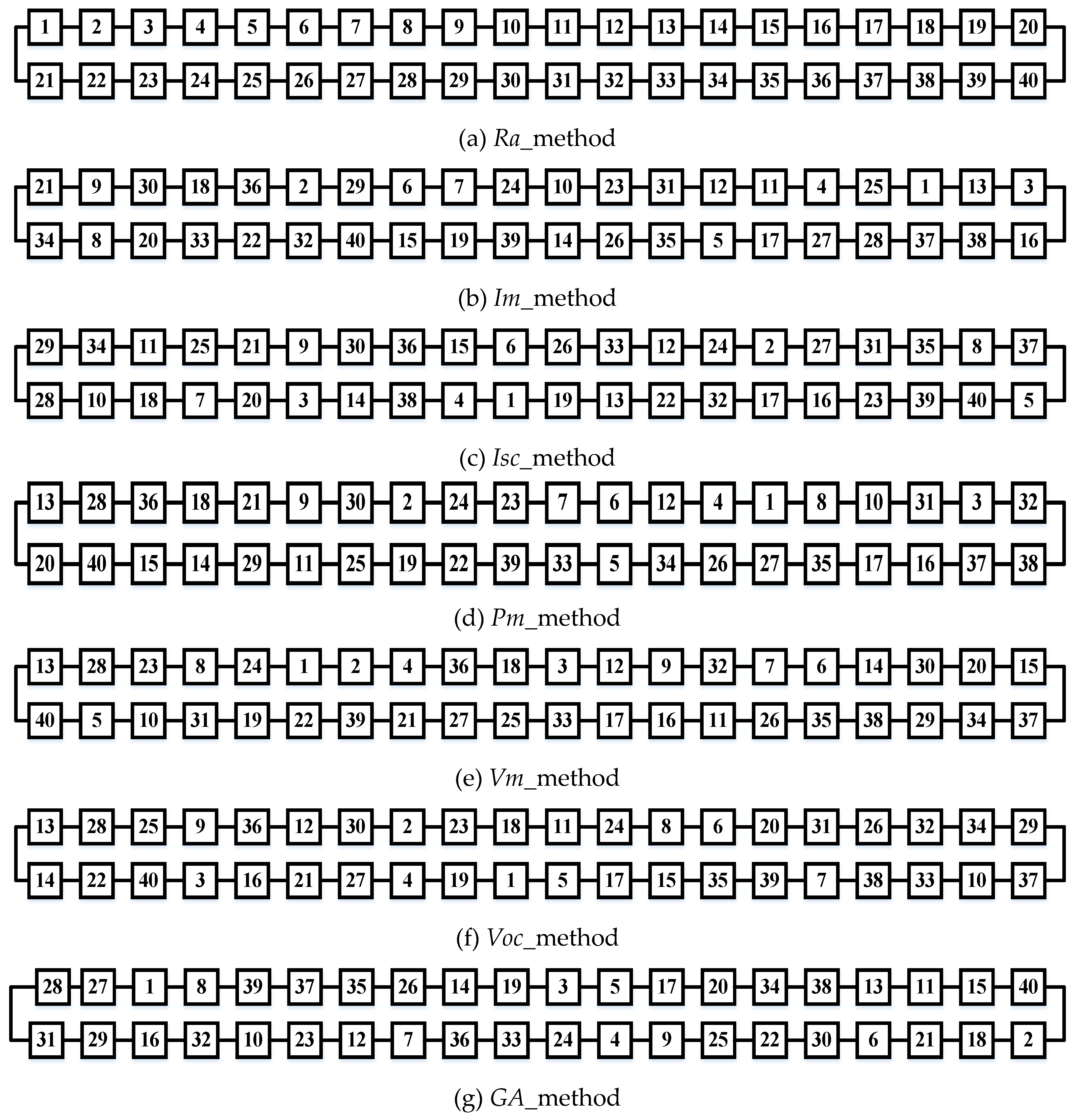
4.2. Conventional Techniques of Module Arrangement

The conventional techniques of SP PV array modules arrangement are based on I-V parameters such as Im, Isc, Pm, Vm or Voc [29,57,58]. Therefore, the arrangement techniques are named according to the selected I-V parameter: i) Im_method; ii) Isc_method; iii) Pm_method; iv) Vm_method and v) Voc_method. For Im based method, let’s consider an LSS-SP array of dimension, 4 × 10 with 40 modules as shown in Figure 5, which are arranged by Im values. The arrangement has been made from lower values to higher values of Im; as a result, module number 1 has the lowest value of Im while module number 40 has the highest. The similar process is also used to arrange the modules by the other methods sated above. The difference of $I_{Module}^{mpp}$ in strings and difference of $V_{Module}^{mpp}$ of strings are the factors causing MML in an array [28,59]. The current-based module arrangement techniques (Im and Isc) minimize MML by greedily reducing the difference of $I_{Module}^{mpp}$ in strings [29,58]. Consequently, the string current ($I_{String}^{mpp}$) increases gradually from the first row to the last row. This arrangement increases the total array current ($I_{Array}^{mpp}$) as in Equation (3) and consequently, the output power increases. The voltage-based modules arrangement techniques (Vm and Voc) reduce the differences of $V_{Module}^{mpp}$ in strings but increases the string voltage ($V_{String}^{mpp}$) from the first row to the last row. Consequently, the array voltage ($V_{Array}^{mpp}$) decreases as in Equation (4). Therefore, the array output power in voltage based methods (Vm and Voc) are comparatively smaller than current based methods (Im and Isc) [28,29]. On the other hand, in power-based method Pm, both array voltage and array current increase averagely, hence the array power increases than voltage-based method but not more than current based method elaborately described in Reference [31]. Another typical technique of module arrangement is the random method (Ra_method), which is mostly used in the small size PV array. In this method, modules are arranged randomly by considering all modules with identical power in the PV array.

4.3. Proposed GA Technique for Module Arrangement

To address the problem of minimizing the MML in SP PV array, GA is used find an optimum arrangement of modules with the expectation that if the array output power can be maximized, the MML will be minimized. Therefore, in this optimization problem, the fitness function of GA is defined as the array output power, $P_{Array}^{mpp}$ that is to be maximized. The expression of the fitness function, FF as follows.

$$FF=P_{Array}^{mpp}.$$

(8)

The total procedure is divided into three steps: selection, crossover, and mutation. Initially, a random number of setups are generated. For generosity, it is considered N numbers of setups are generated. By setup, it means a matrix of r × c consisting of a fixed number of modules. Where ‘r’ is the number of rows, and ‘c’ is the number of columns. Each setup is a sample in the solution space of the optimization problem. The objective of the problem is to find out the best sample with maximum fitness value. The process is illustrated with a flowchart shown in Figure 3.

As in the flowchart in Figure 6, it is started with the phase of selection. In the selection phase, parent samples are selected through some criterion function. In this case, the criterion function is the average of the fitness values of the samples generated randomly. If any sample has a fitness greater or equal to the average of the fitness values of the samples, it is selected as a parent of the current generation. Initially, the average value of the fitness function of the samples is termed as global best, BG. Usually, this process reduces the population size to less than N.

Now, in the following phase known as crossover, it crosses the parent samples and generated new samples. However, the newly generated samples are included in the current generation if they excel in fitness value compared to the best fitness value of the parent samples. The best fitness value of the current parent samples is termed as local best, ‘BL’. The process is terminated when the population size is increased to N again. While selecting a pair of parents for crossover, Roulette wheel selection is used [35].

If FF_i is the fitness of an individual sample, ‘i’ in the population, its probability of being selected is as follows:

$$P_i=\frac{F{F}_i}{{\displaystyle \sum _{j=1}^{N}F{F}_j}}$$

(9)

where ‘N’ denotes as the number of individuals in the population, while any candidate solution with a higher fitness will make less likely to be eliminated, there is still a chance that they may be. Again, with this type of selection, there is a chance some weaker solutions may survive the selection process which serves as an advantage. These retain some feeble properties of weak solutions those could prove useful in the following steps.

For the crossover phase, the order one crossover technique is used in this work because of its simplicity and faster operation. To the best of the author knows, this is the first-time order one crossover technique has been applied to this type of GA based optimal process of module arranged in an SP PV array. During the crossover process, after generating every child sample, a small mutation at a rate of ‘m’ is introduced. This threshold is tuned during simulations. Finally, the procedure stops whenever the global best, ‘BG’ is stabilized for a predefined number of iterations. Otherwise, the current population is again reassessed using the selection procedure and passed through the crossover and mutation phases until the stopping criterion is met. The GA process takes a data set of PV modules with a determined row-column dimension and returns an optimal arrangement of modules position in the array as output.

5. Simulation Result Analysis

5.1. Case Study on a 400 W PV Array

In this section, seven different methods (Ra_method, Vm_method, Voc_method, Pm_method, Isc_method, Im_method, and GA_method) are applied on a 400 W PV array with 40 modules of 10 W each for arranging the modules accordingly to get maximum array output power. Figure 7 shows the optimal arrangement of modules is obtained for LSS-SP (2 × 20) array arrangements using conventional techniques (a–f) and the proposed GA technique (g). The same methods are also performed for 1 × 40, 2 × 20, 4 × 10, 5 × 8, 40 × 1, 20 × 2, 10 × 4, and 8 × 5 array configurations and simulation results of array output power are calculated using a mathematical model described in Section 3. The array output power is depicted in

Table 2. Array output power for 400 W LSS-SP array configurations.

Array Size	Array Output Power (W) by Using Different Techniques for 400 W LSS-SP Array
	Ra_method	Vm_method	Voc_method	Pm_method	Isc_method	Im_method	GA_method
1 × 40	398.125	398.125	398.125	398.125	398.125	398.125	398.125
2 × 20	396.659	396.499	398.072	397.711	398.341	401.544	402.067
4 × 10	395.028	395.132	396.728	397.978	400.086	402.693	403.059
5 × 8	394.340	394.476	396.086	397.630	400.228	403.754	403.785

for four different LSS-SP array arrangments (1 × 40, 2 × 20, 4 × 10, 5 × 8). The results show that power generation by arranging module using GA based method is the maximum for all array arrangements and the maximum array power is 403.785 W for the 5 × 8 array arrangement. An interesting observation is that for a 1 × 40 array arrangement, the array power remains the same for all techniques because the array voltage and the array current remain same arrangement. 4 × 10 and 5 × 8 array arrangements are generating different output power for different methods, and the result shows that the current based methods (Im and Isc) are producing more power than voltage-based methods (Vm and Voc).

Table 3. Array output power for 400 W LPB-SP array configurations.

Array Size	Array Output Power (W) by Using Different Techniques for 400 W LPB-SP Array
	Ra_method	Vm_method	Voc_method	Pm_method	Isc_method	Im_method	GA_method
40 × 1	383.643	383.643	383.643	383.643	383.643	383.643	383.643
20 × 2	392.090	383.978	383.978	385.219	394.482	394.657	398.356
10 × 4	391.648	391.166	393.361	393.845	397.598	400.556	402.729
8 × 5	392.807	392.503	395.221	395.821	399.553	401.379	402.827

shows the array output power for four different LPB-SP array arrangements (40 × 1, 20 × 2, 10 × 4, and 8 × 5). Where the 8 × 5 array output power is 402.827 W, which is the maximum power generated by using GA based method. The array power remains the same for a 40 × 1 array arrangement. Though the power generation by Pm based technique is higher than voltage-based methods (Vm, Voc) but it is lower than the current based methods (Im, Isc) both for LSS-SP and LPB-SP array arrangements. By comparing Table 2 and Table 3, LSS-SP arrays output powers are always higher than LPB-SP arrays for the corresponding module arrangement techniques. However, the lowest array output power 383.643 W is obtained for the 40 × 1 array arrangement.

Figure 8 shows the %MML in the 400 W array both for LSS-SP (1 × 40, 2 × 20, 4 × 10, 5 × 8) and LPB-SP (40 × 1, 20 × 2, 10 × 4, 8 × 5) array arrangements are obtained by using different module arrangement methods. In one hand, minimum %MML are achieved by GA based method both for LSS-SP and LPB-SP array arrangements and the minimum values are 0.94% and 1.18% for 5 × 8 and 8 × 5 arrays, respectively. On the other hand, the Vm based method gives a higher %MML for 20 × 2, 10 × 4, 8 × 5 and 2 × 20 array arrangements. For the 4 × 10 and 5 × 8 array arrangements the random method gives even more %MML than the Vm based method. However, for the 1 × 40 and 40 × 1 array arrangements the %MML are unchanged for all the methods and the maximum MML obtained is 5.89% in 40 × 1 array arrangements. Though the %MML obtained by all techniques are following a similar pattern for LPB-SP (20 × 2, 10 × 4, and 8 × 5) array arrangements as shown in Figure 8, the values of %MML for LPB-SP array arrangements are always higher than LSS-SP array arrangements for each method.

5.2. Case Study on 3400 W PV Array

A 3400 W PV array is made by using 40 modules of 85 W rating using the datasets from Table 1. The array is arranged in 1 × 40, 2 × 20, 4 × 10, 5 × 8, 40 × 1, 20 × 2, 10 × 4, and 8 × 5 array arrangements by using all seven module arrangement methods. The corresponding array power is calculated and tabulated in

Table 4. Array output power for 3400 W LSS-SP array configurations.

Array Size	Array Output Power (W) by Using Different Techniques for 3400 W LSS-SP Array
	Ra_method	Vm_method	Voc_method	Pm_method	Isc_method	Im_method	GA_method
1 × 40	3415.950	3415.950	3415.950	3415.950	3415.950	3415.950	3415.950
2 × 20	3405.038	3405.528	3409.419	3412.54	3418.861	3422.724	3424.072
4 × 10	3402.887	3401.572	3405.725	3412.003	3419.048	3425.178	3426.417
5 × 8	3403.273	3400.943	3405.158	3408.437	3414.527	3426.038	3427.430

and

Table 5. Array output power for 3400 W LPB-SP array configurations.

Array Size	Array Output Power (W) by Using Different Techniques for 3400 W LPB-SP Array
	Ra_method	Vm_method	Voc_method	Pm_method	Isc_method	Im_method	GA_method
40 × 1	3407.484	3407.484	3407.484	3407.484	3407.484	3407.484	3407.484
20 × 2	3410.415	3405.485	3410.201	3406.900	3409.463	3414.522	3426.913
10 × 4	3407.268	3403.179	3406.017	3411.639	3412.906	3424.642	3425.935
8 × 5	3405.368	3401.627	3406.7	3408.674	3415.815	3425.138	3426.92

. The results are similar like 400 W array because the GA based method is again performed better by generating higher array power than all other methods. While Vm based method shows poor performances by generating lower output power for almost all array arrangements. The highest output power, 3427.43 W is obtained by 5 × 8 array arrangement using GA based method and the lowest output power, 3400.94 W is received by Vm based technique for the same array. For 8 × 5 array arrangement by GA based technique output power is 3425.13 W which is the maximum and by Vm based technique output is 3401.62 W which is the minimum. By comparing Table 4 and Table 5 results show that GA based technique is superior for both LSS-SP and LPB-SP array arrangements. However, LSS-SP arrangements are generating more output power than LPB-SP array arrangements.

The %MML in 3400 W PV array for LSS-SP arrays (1 × 40, 2 × 20, 4 × 10, 5 × 8) and LPB-SP arrays (40 × 1, 20 × 2, 10 × 4, 8 × 5) are illustrated in Figure 9. Figure 9 shows that the GA based module arrangement method is performed as the best method for both LSS-SP and LPB-SP array arrangements. The minimum MML is 0.41% and 0.42% obtained by the GA method for 5 × 8 and 8 × 5 array respectively. The Vm based method shows higher %MML for both LSS-SP and LPB-SP array arrangements. The highest values are 1.176% and 1.156% for 5 × 8 and 8 × 5 array arrangements respectively obtained by Vm based method.

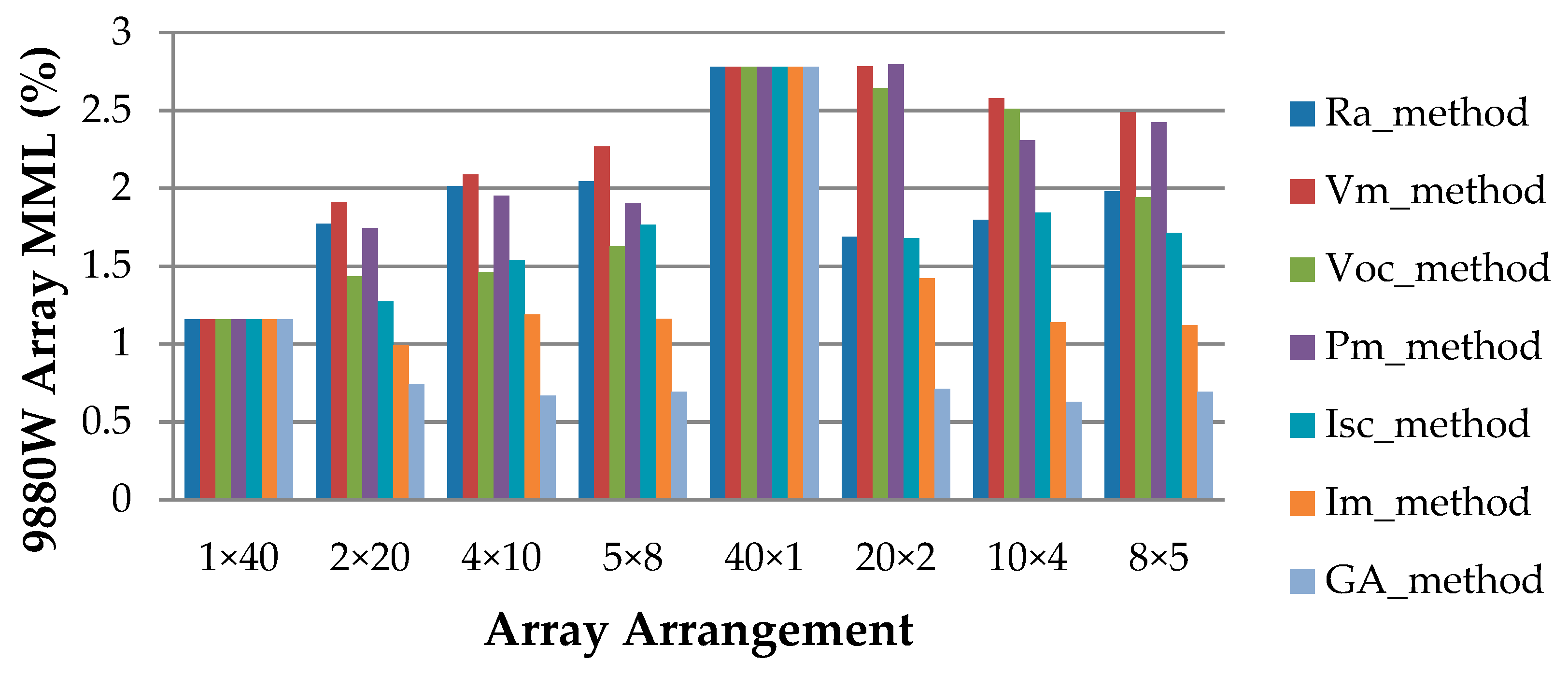
5.3. Case Study on 9880 W PV Array

In this section, module arrangement methods are investigated on a 9880 W PV array. A 9880 W array is developed by using 40 modules of 247 W using datasets from Table 1. At first, 9880 W array is arranged in LSS-SP arrangements (1 × 40, 2 × 20, 4 × 10, 5 × 8) and LPB-SP array arrangements (40 × 1, 20 × 2, 10 × 4, 8 × 5) by using all module arrangement techniques. After that, array output power is calculated by simulation and tabulated in

Table 6. Array output power for 9880 W LSS-SP array configurations.

Array Size	Array Output Power (W) by Using Different Techniques for the 9880 W LSS-SP Array
	Ra_method	Vm_method	Voc_method	Pm_method	Isc_method	Im_method	GA_method
1 × 40	9769.912	9769.912	9769.912	9769.912	9769.912	9769.912	9769.912
2 × 20	9709.074	9695.554	9742.637	9712.042	9758.631	9786.046	9810.914
4 × 10	9685.239	9678.068	9740.016	9691.434	9732.185	9766.97	9818.371
5 × 8	9682.299	9660.148	9723.505	9696.234	9709.943	9769.702	9816.904

and

Table 7. Array output power for 9880 W LPB-SP array configurations.

Array Size	Array Output Power (W) by Using Different Techniques for the 9880 W LPB-SP Array
	Ra_method	Vm_method	Voc_method	Pm_method	Isc_method	Im_method	GA_method
40 × 1	9609.63	9609.63	9609.63	9609.63	9609.63	9609.63	9609.63
20 × 2	9717.518	9609.245	9622.994	9608.048	9718.273	9743.883	9814.136
10 × 4	9706.703	9629.607	9636.243	9656.269	9702.061	9771.7	9822.291
8 × 5	9688.570	9638.369	9692.488	9644.886	9715.177	9773.501	9815.887

. For 1 × 40 and 40 × 1 array arrangements the output power is 9769.91 W and 9609.63 W, respectively. Table 6 shows that the GA based method has a significant role to generate maximum output power for 2 × 20, 4 × 10, and 5 × 8 array arrangements. While the Vm based method generates the lowest output power for the same array arrangements. In this case, the highest array output power is 9818.371 W obtained by the GA based method for 4 × 10 array arrangement. The lowest array output power is 9660.148 W obtained by Vm based technique for 5 × 8 array arrangement.

Table 7 shows that maximum output power is achieved by GA based method for 20 × 2, 10 × 4 and 8 × 5 array arrangements and minimum output powers are obtained by Vm based method for the same array arrangements. The highest power is 9822.291 W in 10 × 4 arrays while the lowest power is 9609.245 W for the 20 × 2 array. By comparing Table 6 and Table 7, it is found that the GA based method is generating higher power than other methods for both LSS-SP and LPB-SP arrays.

For both LSS-SP and LPB-SP array arrangements of 9880 W array, the %MML are illustrated in Figure 10. Figure 10 shows that %MML is always higher for Vm based method and the higher value is 2.78 % for 20 × 2 array arrangements. The lowest value is 0.628 % for 10 × 4 array obtained by GA based method. The lower values of MML are 0.66 % and 0.69 % also acquired for 4 × 10 and 8 × 5 array arrangements respectively by GA based technique. Figure 6 shows that the highest MML is 2.8% achieved by the Pm based technique for 20 × 2 arrays. However, the LSS-SP array arrangements are performed better than LPB-SP array arrangements for GA based method to lower %MML. The current based methods (Im and Isc) are also performed better for both LSS-SP (2 × 20, 4 × 10, 5 × 8) and LPB-SP (20 × 2, 10 × 4, 8 × 5) array arrangements with lower %MML than the random (Ra) and the power-based method (Pm).

5.4. Comparative Analysis of MML in 400 W, 3400 W, and 9880 W Systems

Figure 11 shows the %MML obtained by GA based method for different array configurations (1 × 40, 2 × 20, 4 × 10, 5 × 8, 40 × 1, 20 × 2, 10 × 4, 8 × 5) of 400 W, 3400 W, and 9880 W arrays. The results show that each array configurations have an influence on the %MML and it follows a similar trend for three different PV power systems. In LSS-SP configurations (1 × 40, 2 × 20, 4 × 10, 5 × 8) the highest %MML is found for the longest LSS-SP array (1 × 40), and the %MML are gradually decreasing with the decreasing number of series modules in the array. Hence, the lowest %MML is obtained for a 5 × 8 array. On the other hand, in LPB-SP array configurations (40 × 1, 20 × 2, 10 × 4, 8 × 5) the highest %MML is found for the longest LPB-SP array (40 × 1), and the %MML is decreasing with decreasing the parallel branches in the array. An interesting observation is found between the %MML and the correlation coefficient of Vm and Im of the corresponding datasets. The correlation coefficient of 400 W, 98800 W, and 3400 W arrays are positive (+0.148), negative (−0.567) and negative (−0.435) respectively. The maximum %MML found in 400 W arrays at positive correlation and the minimum is in 3400 W arrays at negative correlation.

Finally, The simulation results show that GA based method is performed better than Im based method for higher output power and lower %MML, while Im is better than Pm and Vm for all three different power ratted arrays (400 W, 3400 W, and 9880 W). Another important observation is that LSS-SP configurations are generating higher power than LPB-SP array configurations. Therefore, these research results will help to take the correct decision about the selection of array size (LSS-SP and LPB-SP) and module rearrangement techniques (GA, Im, Pm, Vm) for future research on this field. The PV system configurations (LSS-SP and LPB-SP) are used basically based on the load voltage and current. For high voltage PV system such as water pumping, grid tie system, LSS-SP is suitable and for a low voltage PV system, such as battery charging for electric vehicles, LPB-SP is suitable. For both the cases, GA and Im based module arrangement techniques can perform better to maximize the array output power.

6. Experimental Validation

In order to validate the simulation results, experimental investigations are carried out using the 400 W array for LSS-SP (4 × 10, 5 × 8) and LPB-SP (10 × 4, 8 × 5) configurations. The experimental setup and the corresponding results are presented in this section.

6.1. Experimental Setup

A 400 W PV array system is composed of 40 poly-crystalline PV modules of 10 W each are placed on the structures with a fixed tilt angle of 23.5°, shown in Figure 12. The array consists of four parallel PV strings of ten PV modules in series. All the PV modules are south facing and are mounted on a rooftop, geographical location of latitude is 23°43′ N and longitude is 90°25′ E, where direct sunlight is available during the daytime. The PV modules are collected from Electro Solar Power Limited with flash test dataset, and their electrical characteristics are already shown in Table 1.

The current-voltage and power-voltage characteristics curves for the 400 W array modules with LSS-SP and LPB-SP configurations are measured and recorded in different atmospheric conditions. To determine the I-V and P-V characteristics, irradiance and temperature corrections are performed according to IEC 60904-1 standard [55].

The I-V and P-V characteristic measurements are performed using the photovoltaic system analyzer (PVSA), PROVA 1011 from the TES Electrical Electronic Corp. The PVSA device measures the electrical characteristics curves of PV module as well as of string or array. It also regulates and calculates efficiency, temperature, irradiance, series resistance of the PV system at outdoor operating condition (OPC). The PVSA device can convert I-V and P-V curves under OPC to data STC based upon IEC standard.

Figure 13 shows the PVSA device, PROVA 1011, a remote solar detector (RSD) 1012 with a thermometer. The analyzer device and RSD rare connected by Bluetooth wireless communication. The RSD device is fully moisture-proof. The maximum power rating of the PVSA device is 12000 W and accuracy for the I-V curve measurement is ±1%.

Table 8. Specifications of the analyzer, irradiance sensor and temperature sensor.

Measurement	Range	Resolution	Accuracy
DC Voltage	1–1000 V	0.01 V/0.1 V/1 V	±1% ± (1% of Voc ± 0.1 V)
DC Current	0.1–12 A	1 mA/10 mA	±1% ± (1% of Isc ± 9 mA)
Irradiance	0–2000 W/m2	1 W/m2	± 3 % ± 20 dgts
Temperature	−22–85 °C	0.1 °C	± 1 % ± 1 °C

shows the technical specifications of the analyzer, Irradiance sensor and temperature sensor. The four-wire to two-wire connecting cables are used to eliminate the systematic errors in voltage measurement, and the measuring interval is 0.02–2 s for a single measure. The PVSA device waits and tests the PV system automatically until appropriate sunlight irradiance is detected.

6.2. Experimental Measurement Procedure

The experimental data measurements of the PV array configurations are carried out in real atmospheric weather conditions throughout the middle of a sunny day and clear sky. By maintaining standard test conditions at outdoor, are described in Reference [60], a single test for I-V characteristics measurement of the PV array is carried out by less than 30 s using the PVSA device, PROVA 1011. As stated by IEC 60904-1 standards [55], photovoltaic I-V characteristic curve measurement can be performed in natural outdoor sunlight during one percent variation of global solar radiation. The incident solar radiation should be at least 800 W/m² [56]. Therefore, in this work, the experimental data recorded within the radiation range between 800 W/m² and 900 W/m² considering no temperature variations. Hence, no temperature correction is proposed in this work. However, the irradiance values are corrected considering 1000 W/m² as the reference irradiance. Consequently, the second procedure of irradiance correction is used in this work, among the three correction procedures proposed in IEC 60891 [56]. The simplified irradiance correction procedure [60] is as follows:

$$I_{mpp}^{reference}=I_{mpp}^{measured}\times \frac{G_{reference}}{G_{measured}}$$

(10)

$$V_{mpp}^{reference}\cong V_{mpp}^{measured}$$

(11)

$$P_{mpp}^{reference}=P_{mpp}^{measured}\times \frac{G_{reference}}{G_{measured}}$$

(12)

where ‘I’ is array current; ‘V’ is array voltage; ‘G’ is irradiance; ‘P’ is array power. The PVSA device is intelligent to measure and store the values of array current, array voltage, array power and irradiance under fast-changing weather conditions. Hence, the reference power in Equation (12) does not represent the maximum power measured at STC. It is the value considered for the performance comparison of array configurations under the same irradiance and temperature conditions.

The objective of the experimental investigation is to record and compare the array output power obtained under different module arrangement methods applied to the LSS-SP (4 × 10, 5 × 8) and LPB-SP (10 × 4, 8 × 5) array configurations. The simulation result shows that the GA based arrangement method and Im based arrangement methods are outperforming than other PV array modules arrangement methods. The random arrangement method is usually used as a conventional PV array module arrangement method. Therefore, these three PV array module arrangement methods are experimentally compared using a 400 W PV array at uniform irradiance condition. Hence shading effects are not considered in this work. All experiments are performed under real operating conditions, and the measured OPC data is processed before being compared using Equation (12). Before each experimental test, the front side of all the PV modules are cleaned, and the module positions are rearranged according to the arrangement results obtained by simulation.

6.3. Experimental Results

In

Table 9. Array output power obtained by experimental work.

Array Configuration	Array Size	400 W Array Output Power Obtained by Experimental Work (W)
		Ra_method	Im_method	GA_method
LSS-SP	4 × 10	378.201	388.110	390.559
	5 × 8	377.06	389.312	392.743
LPB-SP	10 × 4	375.421	386.502	388.648
	8 × 5	376.733	386.919	389.781

, the experimental array output power is obtained for four different array configurations (4 × 10, 5 × 8, 10 × 4 and 8 × 5) using three techniques. Maximum output power was obtained using GA based arrangement for all these array configurations, and the highest power of 392.559 W is obtained in a 5 × 8 configuration. Besides, the Im based technique also performed well by generating higher output power than Ra_method. However, the output power is lower than that obtained using the GA method. Hence, the %RE is calculated with respect to the most conventional Ra_method of module arrangement. Therefore, %RE by Im based method, (%RE_Im), and %RE by GA based method (%RE_GA) are calculated for both Im and GA based techniques, comparing with random based arrangement technique as follows.

$$\%RE\_Im=\frac{P\_Im-P\_Ra}{P\_Ra}\times 100$$

(13)

$$\%RE\_GA=\frac{P\_GA-P\_Ra}{P\_Ra}\times 100$$

(14)

where P_Ra, P_Im, and P_GA are denoted as PV array output power measured by arranging modules using the random method, Im method, and GA method, respectively. The calculated values of %RE_Im and %RE_GA are tabulated in

Table 10. Comparison of recoverable energy between Im based method and GA based method.

Array Configuration	Array Size	Recoverable Energy Obtained by Experimental Work
		%RE_Im	%RE_GA
LSS-SP	4 × 10	2.620	3.267
	5 × 8	3.249	4.159
LPB-SP	10 × 4	2.951	3.523
	8 × 5	2.703	3.463

for both LSS-SP (4 × 10, 5 × 8) and LPB-SP (10 × 4, 8 × 5) configurations. The minimum and maximum value of %RE_Im are 2.62 % and 3.249 %, respectively. On the other hand, by the GA method, the minimum and maximum amount of %RE_GA are 3.267% and 4.159%, respectively. In both cases, the maximum values are obtained by LSS-SP (5 × 8) configuration. The result shows that average %RE obtained by LSS-SP configuration is higher than LPB-SP configurations for both Im and GA based techniques. The average %RE obtained by Im method is 2.88%, and by GA method is 3.60%. Therefore, the GA based technique is performed better than Im based technique for both LSS-SP and LPB-SP configurations.

The %MML obtained by the experimental work for 400 W array is shown in Figure 14. The experimental %MML for LSS-SP (4 × 10, 5 × 8) and LPB-SP (10 × 4, 8 × 5) configurations are calculated by using Equation (7). Where the value of modules power is used 407.63 W, as used in the simulation and the array output power is used from Table 9 for each array configuration. The experimental results show that the minimum %MML are obtained by GA based method both for LSS-SP and LPB-SP configurations which is similar to simulation results.

7. Conclusions

In this work, a new technique of module sorting of PV arrays using GA is experimentally validated both for LSS-SP (4 × 10, 5 × 8) and LPB-SP (10 × 4, 8 × 5) configurations in minimizing MML. The performance of the proposed GA technique regarding total output power and %MML are compared with other conventional module sorting techniques. The conventional current-based methods (Im, Isc) show better performance than the voltage-based methods (Vm, Voc); however, the proposed technique outperforms the conventional ones in every array configuration. The GA technique minimizes the MML by maximizing the array output power, thus increases %RE, both for LSS-SP and LPB-SP array configurations. Additionally, it is observed that the LSS-SP configurations are providing significantly lower %MML than the LPB-SP configurations.

References

1. Hu, Y.; Zhang, J.; Wu, J.; Cao, W.; Tian, G.Y.; Kirtley, J.L. Efficiency improvement of nonuniformly aged PV arrays. IEEE Trans. Power Electron. 2017, 32, 1124–1137. [Google Scholar] [CrossRef]
2. Osório, G.J.; Shafie-khah, M.; Lujano-Rojas, J.M.; Catalão, J.P. Scheduling Model for Renewable Energy Sources Integration in an Insular Power System. Energies 2018, 11, 144. [Google Scholar] [CrossRef]
3. Zhang, T.; Xie, L.; Li, Y.; Mallick, T.; Wei, Q.; Hao, X.; He, B. Experimental and Theoretical Research on Bending Behavior of Photovoltaic Panels with a Special Boundary Condition. Energies 2018, 11, 3435. [Google Scholar] [CrossRef]
4. Ren, G.; Zhao, X.; Zhan, C.; Jin, H.; Zhou, A. Investigation of the Energy Performance of a Novel Modular Solar Building Envelope. Energies 2017, 10, 880. [Google Scholar] [CrossRef]
5. Zhang, T.; Wang, M.; Yang, H. A Review of the Energy Performance and Life-Cycle Assessment of Building-Integrated Photovoltaic (BIPV) Systems. Energies 2018, 11, 3157. [Google Scholar] [CrossRef]
6. Lotfy, M.E.; Senjyu, T.; Farahat, M.A.-F.; Abdel-Gawad, A.F.; Matayoshi, H. A polar fuzzy control scheme for hybrid power system using vehicle-to-grid technique. Energies 2017, 10, 1083. [Google Scholar] [CrossRef]
7. Subramani, G.; Ramachandaramurthy, V.K.; Padmanaban, S.; Mihet-Popa, L.; Blaabjerg, F.; Guerrero, J.M. Grid-tied photovoltaic and battery storage systems with Malaysian electricity tariff—A review on maximum demand shaving. Energies 2017, 10, 1884. [Google Scholar] [CrossRef]
8. Su, M.; Luo, C.; Hou, X.; Yuan, W.; Liu, Z.; Han, H.; Guerrero, J.M. A Communication-Free Decentralized Control for Grid-Connected Cascaded PV Inverters. Energies 2018, 11, 1375. [Google Scholar] [CrossRef]
9. Viinamäki, J.; Kuperman, A.; Suntio, T. Grid-forming-mode operation of boost-power-stage converter in PV-generator-interfacing applications. Energies 2017, 10, 1033. [Google Scholar] [CrossRef]
10. Priyadarshi, N.; Padmanaban, S.; Mihet-Popa, L.; Blaabjerg, F.; Azam, F. Maximum Power Point Tracking for Brushless DC Motor-Driven Photovoltaic Pumping Systems Using a Hybrid ANFIS-FLOWER Pollination Optimization Algorithm. Energies 2018, 11, 1067. [Google Scholar] [CrossRef]
11. Jeong, D.-K.; Kim, H.-S.; Baek, J.-W.; Kim, H.-J.; Jung, J.-H. Autonomous Control Strategy of DC Microgrid for Islanding Mode Using Power Line Communication. Energies 2018, 11, 924. [Google Scholar] [CrossRef]
12. Tubniyom, C.; Chatthaworn, R.; Suksri, A.; Wongwuttanasatian, T. Minimization of Losses in Solar Photovoltaic Modules by Reconfiguration under Various Patterns of Partial Shading. Energies 2019, 12, 24. [Google Scholar] [CrossRef]
13. Gomez, A.; Sanchez, S.; Campoy-Quiles, M.; Abate, A. Topological distribution of reversible and non-reversible degradation in perovskite solar cells. Nano Energy 2018, 45, 94–100. [Google Scholar] [CrossRef]
14. Udenze, P.; Hu, Y.; Wen, H.; Ye, X.; Ni, K. A Reconfiguration Method for Extracting Maximum Power from Non-Uniform Aging Solar Panels. Energies 2018, 11, 2743. [Google Scholar] [CrossRef]
15. Kropp, T.; Schubert, M.; Werner, J.H. Quantitative Prediction of Power Loss for Damaged Photovoltaic Modules Using Electroluminescence. Energies 2018, 11, 1172. [Google Scholar] [CrossRef]
16. Gasparin, F.P.; Bühler, A.J.; Rampinelli, G.A.; Krenzinger, A. Statistical analysis of I–V curve parameters from photovoltaic modules. Sol. Energy 2016, 131, 30–38. [Google Scholar] [CrossRef]
17. Garrido-Alzar, C. Algorithm for extraction of solar cell parameters from I–V curve using double exponential model. Renew. Energy 1997, 10, 125–128. [Google Scholar] [CrossRef]
18. Ciulla, G.; Brano, V.L.; Cellura, M.; Franzitta, V.; Milone, D. A finite difference model of a PV-PCM system. Energy Procedia 2012, 30, 198–206. [Google Scholar] [CrossRef]
19. Franzitta, V.; Orioli, A.; Gangi, A.D. Assessment of the Usability and Accuracy of Two-Diode Models for Photovoltaic Modules. Energies 2017, 10, 564. [Google Scholar] [CrossRef]
20. Franzitta, V.; Orioli, A.; Di Gangi, A. Assessment of the usability and accuracy of the simplified one-diode models for photovoltaic modules. Energies 2016, 9, 1019. [Google Scholar] [CrossRef]
21. Babu, B.C.; Gurjar, S. A novel simplified two-diode model of photovoltaic (PV) module. IEEE J. Photovolt. 2014, 4, 1156–1161. [Google Scholar] [CrossRef]
22. Bany, J.; Appelbaum, J.; Braunstein, A. The influence of parameter dispersion of electrical cells on the array power output. IEEE Trans. Electron. Devices 1977, 24, 1032–1040. [Google Scholar] [CrossRef]
23. Gonzalez Montoya, D.; Bastidas-Rodriguez, J.D.; Trejos-Grisales, L.A.; Ramos-Paja, C.A.; Petrone, G.; Spagnuolo, G. A Procedure for Modeling Photovoltaic Arrays under Any Configuration and Shading Conditions. Energies 2018, 11, 767. [Google Scholar] [CrossRef]
24. Ji, D.; Zhang, C.; Lv, M.; Ma, Y.; Guan, N. Photovoltaic Array Fault Detection by Automatic Reconfiguration. Energies 2017, 10, 699. [Google Scholar] [CrossRef]
25. Serna-Garcés, S.I.; Bastidas-Rodríguez, J.D.; Ramos-Paja, C.A. Reconfiguration of Urban Photovoltaic Arrays Using Commercial Devices. Energies 2016, 9, 2. [Google Scholar] [CrossRef]
26. Saha, H.; Bhattacharya, G.; Mukherjee, D. Mismatch losses in series combinations of silicon solar cell modules. Sol. Cells 1988, 25, 143–153. [Google Scholar] [CrossRef]
27. Bishop, J. Computer simulation of the effects of electrical mismatches in photovoltaic cell interconnection circuits. Sol. Cells 1988, 25, 73–89. [Google Scholar] [CrossRef]
28. Bucciarelli, L.L., Jr. Power loss in photovoltaic arrays due to mismatch in cell characteristics. Sol. Energy 1979, 23, 277–288. [Google Scholar] [CrossRef]
29. Webber, J.; Riley, E. Mismatch loss reduction in photovoltaic arrays as a result of sorting photovoltaic modules by max-power parameters. ISRN Renew. Energy 2013, 2013, 327835. [Google Scholar] [CrossRef]
30. Lorente, D.G.; Pedrazzi, S.; Zini, G.; Dalla Rosa, A.; Tartarini, P. Mismatch losses in PV power plants. Sol. Energy 2014, 100, 42–49. [Google Scholar] [CrossRef]
31. Shirzadi, S.; Hizam, H.; Wahab, N.I.A. Mismatch losses minimization in photovoltaic arrays by arranging modules applying a genetic algorithm. Sol. Energy 2014, 108, 467–478. [Google Scholar] [CrossRef]
32. Deshkar, S.N.; Dhale, S.B.; Mukherjee, J.S.; Babu, T.S.; Rajasekar, N. Solar PV array reconfiguration under partial shading conditions for maximum power extraction using genetic algorithm. Renew. Sustain. Energy Rev. 2015, 43, 102–110. [Google Scholar] [CrossRef]
33. Rajan, N.A.; Shrikant, K.D.; Dhanalakshmi, B.; Rajasekar, N. Solar PV array reconfiguration using the concept of Standard deviation and Genetic Algorithm. Energy Procedia 2017, 117, 1062–1069. [Google Scholar] [CrossRef]
34. Camarillo-Peñaranda, J.R.; Ramírez-Quiroz, F.A.; González-Montoya, D.; Bolaños-Martínez, F.; Ramos-Paja, C.A. Reconfiguration of photovoltaic arrays based on genetic algorithm. Revista Facultad de Ingeniería Universidad de Antioquia 2015, 75, 95–107. [Google Scholar] [CrossRef]
35. Harrag, A.; Messalti, S. Adaptive GA-based reconfiguration of photovoltaic array combating partial shading conditions. Neural Comput. Appl. 2018, 30, 1145–1170. [Google Scholar] [CrossRef]
36. Tazehkand, M.Z.; Fathi, S.H.; Eskandari, A.; Milimonfared, J. Optimal reconfiguration of PV modules in an array without any constraint on structure by the use of genetic algorithm. In Proceedings of the 2018 9th Annual Power Electronics, Drives Systems and Technologies Conference (PEDSTC), Tehran, Iran, 13–15 February 2018; pp. 145–150. [Google Scholar]
37. Chen, P.-Y.; Chao, K.-H.; Liao, B.-J. Joint Operation between a PSO-Based Global MPP Tracker and a PV Module Array Configuration Strategy under Shaded or Malfunctioning Conditions. Energies 2018, 11, 2005. [Google Scholar] [CrossRef]
38. Deline, C.; Marion, B.; Granata, J.; Gonzalez, S. A performance and economic analysis of distributed power electronics in photovoltaic systems. Contract 2011, 303, 275–3000. [Google Scholar]
39. Teo, J.; Tan, R.; Mok, V.; Ramachandaramurthy, V.; Tan, C. Impact of Partial Shading on the PV Characteristics and the Maximum Power of a Photovoltaic String. Energies 2018, 11, 1860. [Google Scholar] [CrossRef]
40. Seyedmahmoudian, M.; Mekhilef, S.; Rahmani, R.; Yusof, R.; Renani, E.T. Analytical modeling of partially shaded photovoltaic systems. Energies 2013, 6, 128–144. [Google Scholar] [CrossRef]
41. Farh, H.; Othman, M.; Eltamaly, A.; Al-Saud, M. Maximum Power Extraction from a Partially Shaded PV System Using an Interleaved Boost Converter. Energies 2018, 11, 2543. [Google Scholar] [CrossRef]
42. Babu, T.S.; Ram, J.P.; Dragičević, T.; Miyatake, M.; Blaabjerg, F.; Rajasekar, N. Particle swarm optimization based solar PV array reconfiguration of the maximum power extraction under partial shading conditions. IEEE Trans. Sustain. Energy 2018, 9, 74–85. [Google Scholar] [CrossRef]
43. Zhao, J.; Zhou, X.; Ma, Y.; Liu, Y. Analysis of Dynamic Characteristic for Solar Arrays in Series and Global Maximum Power Point Tracking Based on Optimal Initial Value Incremental Conductance Strategy under Partially Shaded Conditions. Energies 2017, 10, 120. [Google Scholar] [CrossRef]
44. Gutiérrez Galeano, A.; Bressan, M.; Jiménez Vargas, F.; Alonso, C. Shading Ratio Impact on Photovoltaic Modules and Correlation with Shading Patterns. Energies 2018, 11, 852. [Google Scholar] [CrossRef]
45. Du, Y.; Yan, K.; Ren, Z.; Xiao, W. Designing localized MPPT for PV systems using fuzzy-weighted extreme learning machine. Energies 2018, 11, 2615. [Google Scholar] [CrossRef]
46. Ramos-Paja, C.; Gonzalez Montoya, D.; Bastidas-Rodriguez, J. Sliding-Mode Control of Distributed Maximum Power Point Tracking Converters Featuring Overvoltage Protection. Energies 2018, 11, 2220. [Google Scholar] [CrossRef]
47. Islam, H.; Mekhilef, S.; Shah, N.; Soon, T.; Seyedmahmousian, M.; Horan, B.; Stojcevski, A. Performance evaluation of maximum power point tracking approaches and photovoltaic systems. Energies 2018, 11, 365. [Google Scholar] [CrossRef]
48. Hammami, M.; Grandi, G. A Single-Phase Multilevel PV Generation System with an Improved Ripple Correlation Control MPPT Algorithm. Energies 2017, 10, 2037. [Google Scholar] [CrossRef]
49. Chang, L.-Y.; Chung, Y.-N.; Chao, K.-H.; Kao, J.-J. Smart Global Maximum Power Point Tracking Controller of Photovoltaic Module Arrays. Energies 2018, 11, 567. [Google Scholar] [CrossRef]
50. Chao, K.-H.; Wu, M.-C. Global maximum power point tracking (MPPT) of a photovoltaic module array constructed through improved teaching-learning-based optimization. Energies 2016, 9, 986. [Google Scholar] [CrossRef]
51. Pei, T.; Hao, X.; Gu, Q. A Novel Global Maximum Power Point Tracking Strategy Based on Modified Flower Pollination Algorithm for Photovoltaic Systems under Non-Uniform Irradiation and Temperature Conditions. Energies 2018, 11, 2708. [Google Scholar] [CrossRef]
52. Koutroulis, E.; Blaabjerg, F. A new technique for tracking the global maximum power point of PV arrays operating under partial-shading conditions. IEEE J. Photovolt. 2012, 2, 184–190. [Google Scholar] [CrossRef]
53. Spertino, F.; Akilimali, J.S. Are Manufacturing IV Mismatch and Reverse Currents Key Factors in Large Photovoltaic Arrays? IEEE Trans. Ind. Electron. 2009, 56, 4520–4531. [Google Scholar] [CrossRef]
54. Zilles, R.; Lorenzo, E. Statistical analysis of current voltage characteristics of PV modules. Int. J. Sol. Energy 1991, 9, 233–239. [Google Scholar] [CrossRef]
55. Standard, I. 60904-1, Photovoltaic Devices, Part 1: Measurement of Photovoltaic Current-Voltage Characteristics; International Electrotechnical Commission: Geneva, Switzerland, 2006; Volume 2. [Google Scholar]
56. Standard, I. 60891. Photovoltaic Devices. Procedures for Temperature and Irradiance Corrections to Measured IV Characteristics; International Electrotechnical Commission: Geneva, Switzerland, 2009. [Google Scholar]
57. Sonnenenergie, D.G.F. Planning and Installing Photovoltaic Systems: A Guide for Installers, Architects and Engineers; Routledge: Abingdon-on-Thames, UK, 2013. [Google Scholar]
58. Bakas, P.; Marinopoulos, A.; Stridh, B. Impact of PV module mismatch on the PV array energy yield and comparison of module, string and central MPPT. In Proceedings of the 2012 38th IEEE Photovoltaic Specialists Conference (PVSC), Austin, TX, USA, 3–8 June 2012; pp. 001393–001398. [Google Scholar]
59. Kaushika, N.; Rai, A.K. An investigation of mismatch losses in solar photovoltaic cell networks. Energy 2007, 32, 755–759. [Google Scholar] [CrossRef]
60. Bana, S.; Saini, R. Experimental investigation on power output of different photovoltaic array configurations under uniform and partial shading scenarios. Energy 2017, 127, 438–453. [Google Scholar] [CrossRef]
Figure 1. Mismatch power loss (MML) in PV array due to modules I-V mismatch at uniform irradiance.
Energies 12 00874 g001
Figure 2. Correlation between Vm and Im of 10 W modules in 400 W array.
Energies 12 00874 g002
Figure 3. Correlation between Vm and Im of 85 W modules in a 3400 W array.
Energies 12 00874 g003
Figure 4. Correlation between Vm and Im of 247 W modules in a 9880 W array.
Energies 12 00874 g004
Figure 5. 4 × 10 LSS-SP array configuration.
Energies 12 00874 g005
Figure 6. Flowchart of the genetic algorithm based PV modules arrangement technique.
Energies 12 00874 g006
Figure 7. 2 × 20 array modules are arranged by: (a) Ra, (b) Im, (c) Isc, (d) Pm, (e) Vm, (f) Voc and (g) GA methods.
Energies 12 00874 g007
Figure 8. MML for LSS-SP and LPB-SP array configurations of 400 W array.
Energies 12 00874 g008
Figure 9. MML for LSS-SP and LPB-SP array configurations of 3400 W array.
Energies 12 00874 g009
Figure 10. MML for LSS-SP and LPB-SP array configurations of 9880 W array.
Energies 12 00874 g010
Figure 11. MML obtained by GA based method for different configurations of 400 W, 3400 W, and 9880 W array.
Energies 12 00874 g011
Figure 12. Experimental setup of 400 W array for comparing maximum array output power using different methods of modules arrangement.
Energies 12 00874 g012
Figure 13. PV system analyzer: (a) PROVA 1011, (b) remote solar detector and (c) thermometer.
Energies 12 00874 g013
Figure 14. MML obtained by an experiment using three different techniques for 400 W array configurations.
Energies 12 00874 g014