Abstract
In the optimized design of power converters, loss analysis of power devices is important. Compared with estimation methods, measuring the power device loss directly in the circuit under test is more accurate. The loss measurement method can be divided into two categories: electrical measurement and calorimetric measurement. The accuracy of the electrical measurement result is restricted to the accuracy of the measurement equipment and parasitic parameters, especially for fast switching devices like SiC devices. The results obtained from calorimetric measurement are more convincing. Based on the measurement principle, calorimetric measurement can be divided into four categories: flow density measurement, temperature equivalent measurement, double jacket measurement, and temperature sensor measurement. This paper proposes an optimized temperature sensor measurement method, which has shorter time consumption, a simpler setup, and lower cost. The principles of the optimized method are described and compared with the traditional ways in detail to show its advantages. The loss measurement and error analysis are carried out in a three-level ANPC (active neutral-point-clamped) topology experiment platform based on the SiC&Si hybrid module to prove the accuracy and practicability of this method.
1. Introduction
Power device loss analysis is an important part of the optimized design of power converters. A general and convenient method is to extract the on-state and switching characteristics from the datasheet provided by the supplier and then estimate the total power device loss through an analytical formula and modeling [1,2]. However, switching loss data are not always available in datasheets. Even if the data are given, the test conditions are inconsistent with the actual circuit operating conditions. Therefore, the error obtained by this estimation method can be very large.
Compared to the analytical results, the power loss measured from the actual operating circuit under test is more convincing. Loss measurement methods can be divided into two categories: electrical measurement and calorimetric measurement. A common electrical measurement method is named the double pulse test [3]: giving the device under test (DUT) a pulse signal and measuring the voltage and current curve during turn-on and turn-off process, integrating them to obtain switching loss. This method requires the insertion of probes for measuring voltage and current in the circuit. The insertion of these probes introduces unnecessary parasitic parameters, which can affect the switching curves of the power devices (especially in the case of high-frequency switches), causing distortion of the measured voltage and current curves. Because the switching process time is very short, this test requires high bandwidth for the measuring equipment. Another commonly-used electrical method in engineering is to measure directly the input and output power of the circuit; the loss of the circuit under test can be obtained by subtraction. In addition to power device losses, the losses measured by this method may also include drive losses, passive device losses, and so on.
Since power loss is dissipated as heat, it can be determined indirectly by measuring the temperature change caused by heat dissipation, which is called calorimetric measurement. According to the different measurement principles, calorimetric measurement can be divided into four categories [4]: flow density measurement, temperature equivalent measurement, double jacket measurement, and temperature sensor measurement. The first type of flow density measurement is obtained by testing the mass flow rate and temperature rise. For example, the method in [5] was to measure the air temperature difference before and after cooling by an air flowmeter and then calculate the corresponding loss through the inherent parameters such as density and specific heat of the air flow. In [6,7], the temperature difference between the inflow and the outflow was measured by a water cooling device. The method in [8] was to measure the temperature difference between the inside and outside of the isolation box. This measurement method needs to know the intrinsic parameters of the selected cooling medium accurately, and the accuracy of the test results is closely related to the accuracy of the measurement device. Therefore, if we want to achieve high-precision test results, the cost of the measurement device can be high. The temperature equivalent measurement needs to design a temperature insulation box with good isolation performance (i.e., heat exchanger) to carry out two experiments, namely calibration experiment and main experiment [9,10,11,12]. In the main test, while the circuit under test is normally operating, the steady temperature of the air in the calorimeter is recorded. Then, in the calibration experiment, the circuit under test stops operating, and heat is accurately injected into the insulation box through a known heater. In calibration experiments, when the steady temperature of the air in the insulation box is the same as the previous main experiment, the power consumed by the circuit under test can be obtained equivalently. However, due to the larger heat capacity of the air, the experimental process has a long time consumption. The two methods mentioned above both require an important measurement device: a temperature isolation box. The better the insulation of the temperature isolation box is, the less the heat loss is, and the higher the accuracy of the measurement results is. Thus, there is a third method called the double jacket test, which is actually an optimum design for the temperature isolation box [13,14].
In order to simplify the measurement device and reduce the cost, the works in [15,16,17,18,19,20,21,22,23,24,25,26] only needed to test the temperature of a certain point through temperature sensors on the power devices with heat sinks to achieve power losses indirectly. We call this method temperature sensor measurement. The measurement device is simple and requires only temperature sensors and DUT with heat sinks. This paper analyzes the principle of this measurement method and compares the advantages and disadvantages of the traditional methods belonging to this category. An optimized temperature sensor measurement method is proposed, where the measurement time consumption is short, the setup is simple, and the cost is low. Therefore, it is more suitable for engineering applications. The measurement method was applied to the SiC&Si hybrid module three-level ANPC single-phase inverter experimental platform, and error analysis was performed. In order to verify the accuracy of this method, an electrical loss measurement was carried out for comparative analysis and verification. In the second section, the principle analysis, advantages, and disadvantages of the traditional measurement methods are described through the thermal-circuit model. The optimized measurement method is proposed. The third section introduces the measurement platform and experimental steps of the proposed optimized measurement method. In the fourth section, the loss measurement of both electrical and calorimetric methods is proposed in a three-level ANPC topology experiment platform based on the SiC&Si hybrid module. Error analysis is also carried out. The fifth section is the conclusion.
2. Temperature Sensor Measurement Method
In this section, we proposed an optimized temperature sensor loss measurement method. In order to highlight the advantages of the proposed method, we demonstrate the principle of the traditional temperature sensor loss measurement method and the optimized method proposed in this paper by establishing a thermal-circuit model of the universally-applicable power device heat dissipation structure. The advantages and disadvantages of these methods are summarized.
2.1. Thermal-Circuit Model and Principle Analysis
In engineering applications, power devices are generally cooled by air-cooled heat sinks. A layer of silicone grease is applied between the bottom of the DUT and heat sink to ensure good thermal contact. In this heat dissipation structure, the DUT is like a heat source, and the heat flux mainly has three conduction paths, as shown in Figure 1a: (1) diffusion into the air through the PCB; (2) diffusion into the air through the outer casing of the DUT; (3) diffusion into the air through the heat sink. The thermal model was established as shown in Figure 1b. In Path (1), the connection between PCB and power device does not fit closely, and there is air thermal resistance in the gap between them. Due to the small thermal conductivity of the air, the air thermal resistance is very large. Thus, there is very little heat flowing through Path (1) and Path (2). In Path (3), the heat sink provides a low thermal resistivity path for the heat produced by DUT. Therefore, Path (3) will flow through most of the heat.
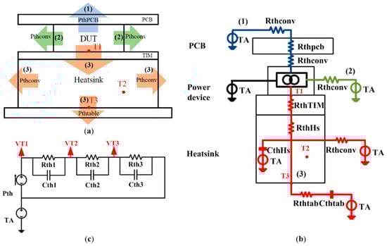
Figure 1.
(a) Schematic diagram of DUT with heat sink; (b) thermal model of DUT with heat sink; (c) simplified thermal-circuit model of DUT with heat sink.
There are usually two strategies to model the thermal behavior of a power electronic module: distributed parameter approach and lumped parameters approach [27]. The Foster-type network topology is one of the lumped parameters approach, which has nothing to do with the actual physical layer and material. The number of thermal resistances and impedances in the Foster model can be determined according to the number of measurement points, and their values are determined by actual measurement. In order to find out the relationship between the power dissipation of DUT and the temperature change, we set three temperature measurement points (, , and ) on Path (3). , , and respectively correspond to: a point on the contact surface of DUT and the heat sink, a point inside the heat sink, and a point on the bottom of the heat sink. The simplified Foster network thermal-circuit model is shown in Figure 1c, where , , and respectively correspond to the voltage values of , , and . In the Foster network thermal-circuit model, represents the power dissipated form DUT, corresponding to the current in the model; represents the ambient temperature, corresponding to the constant voltage source in the model; ~ and ~ respectively represent thermal resistance and capacitance between and , and , and and , corresponding to the resistance and capacitance in the model. , , and can be expressed as:
where () denotes the transient thermal impedances, which are RC low-pass circuits constructed by thermal resistance () and thermal capacitance () of the corresponding part. () can be expressed as:
The time constant () is similar to that defined in electrical engineering.
The transient process time of () is (), which represents the time reaching the final value of 0~99.3%. When the time exceeds or the value reaches 99.3%, it is regarded as the steady state (thermal balance) conditions, that is equal to the final value. The steady state values are , , and respectively. As for a fixed power device with heat sink, the value of the thermal impedance of each part is also fixed. Then, there are one-to-one correspondences between the steady state value of , , , and . The relationship between the steady state value of , , , and can be plotted through a calibration experiment. Then, in the actual circuit loss measurement experiment, the power loss can be obtained through temperature measuring.
2.2. Traditional Temperature Sensor Measurement Methods
According to the difference between the temperature measurement point positions and the temperature data processing methods, the traditional measurement methods based on the temperature sensor can be divided into two categories. One is to achieve the relationship between the steady state temperature and the power dissipated by DUT. We call this method steady state temperature measurement. As in [17], by measuring the steady state temperature of the intersection of the heat sink and DUT (referred to as in Figure 1), the loss of the DUT can be achieved indirectly. The steady state temperature can also be measured at and . In addition to the temperature measurement points on the main heat-dissipation path mentioned above, some temperature sensors are set at other locations. In [19], the steady state temperature point was on the heat dissipation path through the PCB (Path (1) shown in Figure 1). Since most of the heat flow of DUT does not pass through this point, when the measured power is low, the temperature change is small. Then, the temperature measurement result error at this point is large. In [23,24,25,26], a heat flow sensor consisting of two thermocouples and a substrate was inserted at the intersection of the heat sink and DUT, and the power loss was obtained indirectly by the temperature difference between the heat flow sensor when the power device with heat sink reaching thermal balance with the environment. For the methods mentioned above, it cost a long time for the temperature to be measured as reaching the steady state value; because the steady state value can only be obtained at the thermal balance between DUT with the heatsink and environment. For example, it took more than one hour to reach the steady state in [17]. The long time consumption limits the wide application in engineering.
However, it was found that when the time to reach the steady state is long, the initial phase of the curve can be approximated as monotonous change. The slope of the monotonic curve is constant, and the amount of change in temperature is the same in the same period. We call this method instantaneous temperature measurement. The methods in [15,18] were to measure the amount of temperature change over a fixed small period of time in the initial phase of and plot the relationship with the given power. The method in [16] was to obtain the relationship between the slope of this approximate monotonic curve and given power. The method in [20,21] was to measure the amount of temperature change in a small period of time in the initial stage of . Compared with steady state temperature measurement, this instantaneous temperature measurement has a relatively short test time. However, since this curve is not actually monotonously changed, in order to obtain an accurate temperature change, the measurement time control is stringent. Moreover, due to the low temperature change of the initial stage of temperature curves, if the accuracy of the temperature measuring device is not high enough, the measurement result may fluctuate, affecting the data processing result. In addition to the above two methods, the work in [22] inserted a semiconductor refrigerating sheet between the heat sink and DUT to measure the heat flux and used the Seebeck and Peltier effect formula to obtain the dissipated power. However, this formula calculation involves the estimation of various parameters, which is complicated and has large errors.
2.3. Optimized Measurement Method: Steady State Temperature Difference Measurement
In the most ideal method, the temperature to be tested can reach the steady state value quickly, and the measurement device used should be simple. By analyzing Equation (1), we find that if they are subtracted from each other, the resulting temperature differences have a smaller steady state value and shorter transition process time. The resulting temperature difference can be expressed as:
Figure 2 shows the schematic diagram of the , , , and change with time, where , , are changed from ambient temperature and is changed from 0. The temperature measured points of the steady state temperature measurement method and instantaneous temperature measurement method are also noted in Figure 2. It can be seen that reaching the steady state value consumed much shorter time. Therefore, we can indirectly measure power loss by obtaining the steady state temperature difference between the top and bottom of the heat sink. In fact, the principle of measuring the temperature difference between a certain point inside the heat sink and the upper or lower sides is the same. Here, the upper and lower surfaces of the heat sink are selected for the convenience of the arrangement of thermocouples. We call this optimized method the steady state temperature difference measurement method. The steady state temperature difference measurement does not need to wait for thermal balance between DUT with the heat sink and environment. The temperature difference to be measured can reach the steady state very quickly. Therefore, this optimized measurement method is fast and stable. The comparison of this method with traditional loss measurement methods is shown in Table 1.
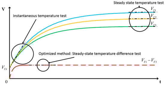
Figure 2.
Schematic diagram of the traditional measurement method and the optimized measurement method.

Table 1.
Comparison of loss measurement methods.
The Foster model of Figure 1c was parameterized in Section 4.2 through actual measurement data. Through simulation, the speedup of the optimized method can be quantified, as shown in Figure 3. It can be seen that in the optimized method, only 240 s were needed to reach the steady state, while the traditional steady state measurement required 1750–2100 s.
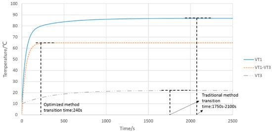
Figure 3.
Simulation diagram of the traditional measurement method and the optimized measurement method.
3. Loss Measurement Device and Experimental Steps
In this section, the available DUT of the proposed method is first explained, and then, the settings of DUT and its heat sink in this experiment are explained. This loss measurement includes two parts: calibration experiments and main experiments. The measurement principle and procedure are described.
3.1. Loss Measurement Device
The commonly-used power devices are discrete devices and power modules, shown in Figure 4a,b. Figure 4c is a power electronic device structure including a DCB (direct copper bonding) substrate. In low-power applications, when the blocking voltage is between 600 V and 1200 V, discrete devices in the TO247 package, power modules, and IPMs (intelligent power modules) are commonly used. IPM refers to power semiconductor modules that integrate electronic circuits that provide additional functions such as drive circuitry and signal processing. For medium-power applications, standard modules dominate. However, in high-power applications, high-reliability IPM modules are more widely used. This loss measurement method is applicable to any discrete device and power module, either individually or collectively. Select the appropriate heat sink according to the size and power level of DUT, and perform calibration experiments, then the power loss can be achieved by the loss measurement experiments.
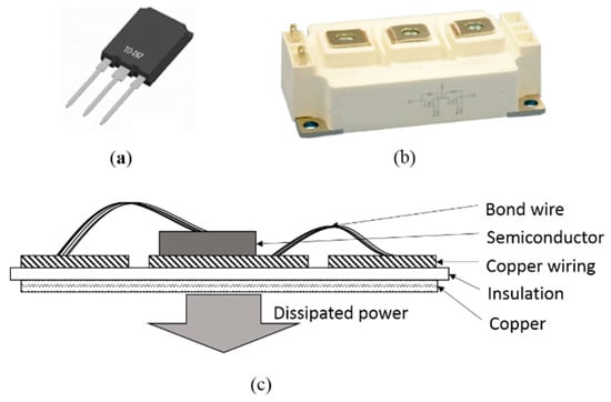
Figure 4.
(a) Discrete device; (b)Power module; (c) Power electronic device structure containing direct copper bonding (DCB) substrate.
In this measurement, we want to analyze the loss distribution of the six discrete devices in the TO247 packages in the ANPC topology, so it is necessary to obtain the losses of the individual switches separately. Therefore, the conventional integral heat sink cannot be used for heat dissipation in this measurement. By analyzing the board layout, discrete device dimensions, and power level for each switch, we designed six copper blocks of 2 cm × 3 cm × 5 cm and fixed them to the bottom of DUT. The measurement device schematic diagram is shown in Figure 5. Common temperature acquisition devices include thermocouples, fiber optic sensors, and thermal imagers. Under normal conditions, thermocouples can achieve temperature measurements well. Fiber optic temperature sensors can achieve better test accuracy in special conditions and environments. The thermal imager is a good way to observe the temperature distribution. In [28], by combining fiber optic sensors with thermal imagers, more specific test results could be obtained. In this experiment, because the position of the temperature points to be measured is not conducive to the placement of fiber optic sensor probes, nor is it suitable for thermal imager observation (temperature test points are coincident in any direction), the thermocouples are used for the temperature test. At the interface between the copper block and DUT, we fixed a thermocouple A. The thermocouple B was fixed at the bottom of the copper block. In this way, we can perform loss measurement by testing the temperature difference between Thermocouples A and B. In addition, since the loss of a single power device is small and the thermal energy converted into the copper block is small, the temperature change is not obvious, which may cause a large temperature test error. Therefore, we wrapped the copper block in a layer of insulation material to reduce the heat loss to the air. Silicone grease was applied between DUT and the copper block and was fixed by a high-temperature-resistant rubber band.
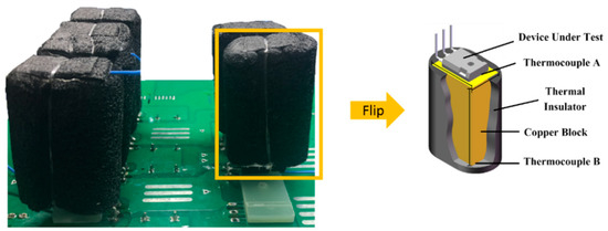
Figure 5.
Loss measurement device.
3.2. Experimental Principles and Steps
This loss measurement includes two parts: calibration experiments and main experiments. The calibration experiment was to obtain the relationship between temperature to be measured and power loss. In this article, the temperature to be measured refers to the temperature difference between the two thermocouples fixed on the upper and lower surfaces of the copper block, shown as:
By inputting known power () to DUT, the corresponding steady state temperature difference () can be obtained. By repeating the above experiment at different powers, we can plot the relationship of and . It can be seen from Equation (3) that in the case where the measurement device is fixed (the thermal impedance value is constant), the relationship between steady state temperature difference and is linear, that is:
where () is the relationship coefficient. The ultimate goal of the calibration experiment was to get as accurate as possible.
First, by simply estimating the power loss of DUT, the approximate power interval can be obtained. The given power should be taken in this interval. Then, according to the on-state voltage given in the datasheet of DUT, the current output range () of the DC source can be estimated. Give a constant conduction signal to the DUT, so that the given current flows through it. Simultaneously measure the on-state voltage () of DUT. The value of the given power is . Simultaneously measure the temperature changes of the upper and lower surfaces of the copper block at a given power . Finally, through data processing, the relationship between and can be obtained. Shown in Figure 6 is the calibration experiment wiring diagram: the constant current source current was directly introduced into the two ends of the DUT, and the multimeter measured its on-state voltage, while the temperature collection was to measure temperatures. The circuit under test was placed in a box to reduce the influence of the external environment on the temperature measuring device.

Figure 6.
Calibration experiment wiring diagram.
Pay attention to the following two points during the calibration experiment. First, during the first calibration experiment, the test time should be slightly longer to determine when the temperature difference reaches steady state. It can be seen from Equation (2) that the time when the temperature difference reaches the steady state at different input powers is the same. In the subsequent experiments, the experimental time can be shortened based on the steady state time obtained in the first calibration experiment. In addition, the position of the thermocouple cannot be changed in the calibration experiment and main experiment. Otherwise, a change in the impedance value in Equation (2) will cause changes in the coefficient of the relationship of and .
In the main experiment, the experiment platform worked normally, and the steady state temperature difference was tested. Corresponding to the calibration curve of and obtained before, the corresponding power can be obtained.
4. Experiment
The loss measurement was operated on a three-level ANPC topology experiment platform based on the SiC&Si hybrid module. This section begins with a brief introduction to the operation of the ANPC topology. Then, the steady state temperature difference versus power curves of each DUT was obtained through calibration experiments, and the comparison verification was carried out through the Foster model simulation. Then, the calorimetric loss measurement was carried out on the three-level ANPC topology experiment platform based on the SiC&Si hybrid module and compared with the results of the electrical power loss measurement; the correctness of the proposed method was proven. Finally, an error analysis was carried out to illustrate the accuracy of this method.
4.1. Operating Principle of the ANPC Topology
The loss measurement was carried out in a three-level ANPC topology experiment platform based on the SiC&Si hybrid module. The single-phase ANPC topology has six switching devices, as shown in Figure 7a. Since the active clamp power devices (T5 and T6) have the ability to flow in both directions, in addition to the P and N output states, the ANPC three-level inverter has four zero-state output modes OU1, OU2, OL1, and OL2. As shown in Table 2. The ANPC topology has two traditional modulation strategies, which we call SPWM1 and SPWM2 [29]. In the SPWM2 modulation, in the positive half cycle of the modulation voltage, when the modulated wave is larger than the upper carrier, the bridge arm outputs the P state; when the modulated wave is smaller than the upper carrier, the bridge arm outputs the OL2 state. In the negative half cycle of the modulation voltage, when the modulated wave is larger than the download wave, the bridge arm outputs the OU2 state; when the modulated wave is smaller than the download wave, the bridge arm outputs the N state. The driving waveform of SPWM2 is shown in Figure 7b. It can be seen that in SPWM2 modulation, the high frequency switching signals are concentrated on T2 and T3. The remaining four switches are power frequency switches. Therefore, the switching losses on T2 and T3 are large, while the remaining four switches have no switching losses. Compared to conventional Si IGBTs, SiC MOSFETs can significantly reduce switching losses. Therefore, we used the SPWM2 modulation and replaced the Si IGBTs of the T2 and T3 with SiC MOSFETs to reduce the total loss.
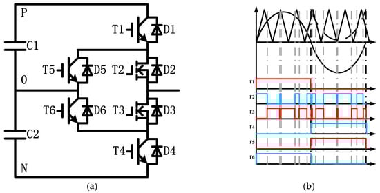
Figure 7.
(a) ANPC topology based on the SiC&Si hybrid module; (b) driving waveform of each tube under SPWM2 modulation.
Table 2.
Switching status of the ANPC three-level inverter.
4.2. Calibration Experiment and Result Analysis
The calibration experiment was first performed. Since the upper and lower arms of the ANPC topology are symmetrical, the calibration experiments were performed on T1, T2, and T5. The T1 loss measurement device is specifically described as an example. In order to eliminate the influence of ambient temperature, the temperature values in Figure 8 were after subtracting the ambient temperature curves. When the input current of the constant current source was set to 0.5 A, the loss of T1 was too small, and the temperature change caused by the heat flow was not obvious. Due to the accuracy limitation of the temperature measuring device, the temperature test point fluctuated (as shown in Figure 8a), which will cause errors in data processing. Therefore, the input power cannot be too small. When the input current was set to 6 A, the temperature change can be measured accurately, as shown in Figure 8b. It can be seen that the temperature difference can reach the steady state at 200 s, so we can reliably extract the steady state temperature difference between 200 s and 300 s. In addition, in this experiment, the heat of DUT flow into the copper block cannot be cooled well like a conventional heat sink (the copper block is wrapped with heat-insulating material), so the operating temperature of DUT should not be too high. When the input current was 6 A, the temperature of the interface between DUT and the copper block reached 70 °C in 300 s. For safety reasons, the maximum input current for the calibration experiment was set at 6 A.
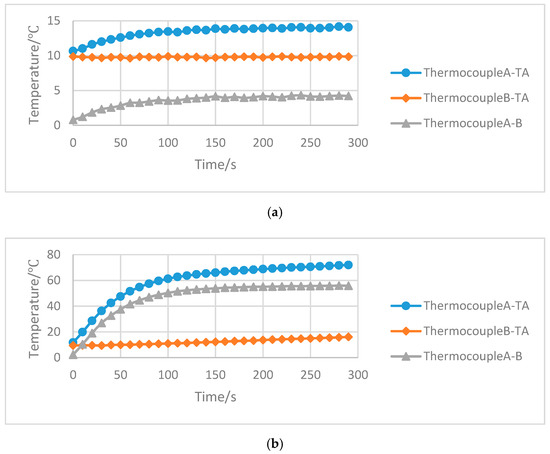
Figure 8.
(a) Thermocouple temperature and temperature difference at 0.5 A; (b) thermocouple temperature and temperature difference at 6 A.
In order to verify the accuracy of the thermal-circuit model (shown in Figure 1c), the temperature measurement result curves at the input current of 6 A were taken to obtain the thermal-circuit model parameters. As for the size of the copper block used in this paper, the given current was large enough. Thus, one set of RC combinations was enough for the modeling of the block. Figure 1c is simplified as shown in Figure 9a. VT1 and VT3 are the locations where thermocouples were placed in the loss measurement set, and the temperature difference was VT1−VT3. Rth1&2, Cth1&2, Rth3, and Cth3 in Figure 9a are the parameters to be determined. When their values were 8.1, 5.5, 1.5, 250, respectively, the simulation results of VT1, VT3, and VT1−VT3 basically coincided with the actual measurement results, as shown in Figure 9b. The time constants of VT1, VT3, and VT1−VT3 were 375, 419.55, and 44.55, respectively. After the parameters were determined, the simulation relationship between the power of T1 and the steady state temperature can be obtained by giving different powers, as shown in Figure 10. The solid point in Figure 10 is the actual experimental measurement result, and the experimental fitting curve is the relationship curve we actually used. It can be seen that the experimental fitting relationship curve was slightly different from the simulation curve, because in the actual measurement, the temperature difference between the upper and lower surfaces of the copper block will not be completely consistent due to the influence of the external heat source (such as an illumination lamp). Therefore, the parameter was used for calibration.
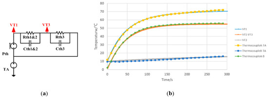
Figure 9.
(a) Simplified thermal-circuit model; (b) simulation and actual temperature curves at 6 A.
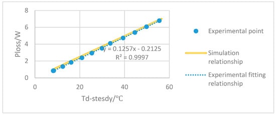
Figure 10.
Simulation and experiment steady state temperature difference versus power of T1.
Similarly, the relationship of T2 and T5 is expressed as:
The values of , , and were different, mainly related to the thermal resistance of the power device itself, the tightness of the connection between copper block and DUT, and the placement of the thermocouples.
4.3. Main Measurement
The ANPC topology was used in the experimental platform, where T2 and T3 were two SiC MOSFETs and the remaining four were Si IGBTs. The Si IGBT was Infineon’s IKW40N120H3, and the SiC MOSFET was Cree’s C2M0080120D. The experimental platform is shown in Figure 11. The load resistor was a 20 Ω ripple resistor; the filter inductor was 0.9 mH. Since the high-frequency switching loss is concentrated on SiC MOSFETs and SiC MOSFET switching loss is small, the switching frequency can be set slightly higher. Furthermore, taking into account the output current harmonics and inductance values, the setting switching frequency cannot be too low; nor can it be too high, because the measurement device has limited heat dissipation capability. Therefore, the final setting was at 40 kHz. Experiments were carried out to measure the losses of T1, T2, and T5 when the DC bus voltage was 250~500 V.
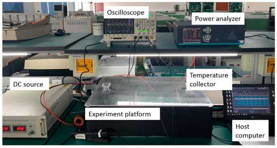
Figure 11.
Experimental platform.
When the bus voltage was input to 500 V, the temperature difference of T1, T2, and T5 between ambient temperatures were as shown in Figure 12. As long as the onset temperature of the temperature difference curve was less than its steady state values, at a particular power, different starting temperatures had no effect on the steady state temperature value. That is to say, we did not need to wait for the DUT and heat sink to cool completely in each experiment, which improved the measurement speed. It can be seen that the temperature difference reached a steady state around 200 s. Therefore, we took the mean of the temperature difference between 200 s and 300 s as the steady state data. The steady state temperature difference values of T1, T2, and T5 under different bus voltages are shown in Table 3. Taking the mean value in Table 3 into Equation (6), the power loss under different bus voltages can be obtained, as shown in Figure 13.
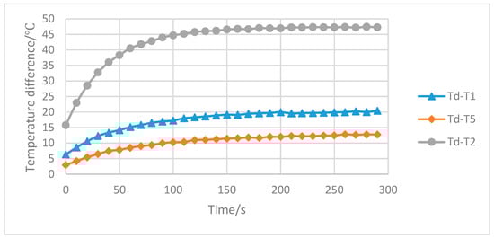
Figure 12.
Temperature difference of T1, T2, and T5 when bus voltage is 500 V.
Table 3.
Td (temperature difference) of T1, T2, and T5 under different bus voltages.
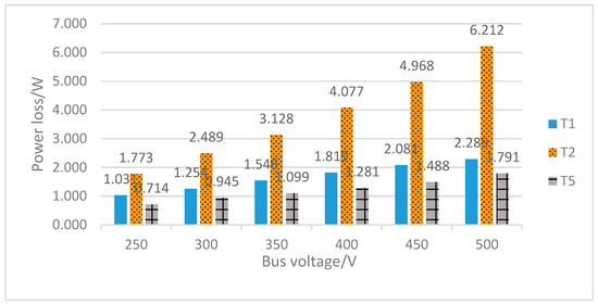
Figure 13.
Loss distribution of T1, T2, and T3 under different bus voltages.
The SiC MOSFET of the T2 (T3) suffered from all the high-frequency switching losses, and as the input voltage increased, the ratio of this loss increased. The remaining four of Si IGBTs were only subjected to on-state losses, and the tendency to increase was similar.
In order to verify the correctness of the calorimetric loss measurement results, we also conducted an electrical measurement. The power analyzer NORMA5000 was used to measure the input and output power of the main circuit, and the two were subtracted to obtain the loss of the main circuit. The loss results of the two measurements were compared at 250 V–500 V, as shown in Table 4. In addition to power device losses, the electrical measurement results included drive circuit losses, DC side voltage equalization capacitance losses, and so on. Therefore, the loss value obtained by the electrical measurement was slightly larger than the calorimetric measurement result, as shown in Figure 14.
Table 4.
Electrical loss measurement results under different bus voltages.
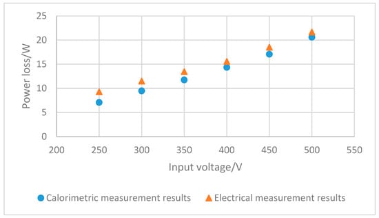
Figure 14.
Comparison of electrical and calorimetric loss measurement results.
4.4. Error Analysis
When a fixed current is set in the DC current source during the calibration experiment, the power dissipation should also be constant. Therefore, in an ideal situation, when the same power is given, the measured steady state temperature difference should also be the same value, and is also a constant value. However, in the actual test, there was an error between the actually obtained power and the steady state temperature difference. The accuracy and reading error of the multimeter and the difference in the fixed position of the measuring terminal will cause the error, that is the error of . In order to reduce the error caused by the fixed position of the measuring terminal of the multimeter, the measuring terminal of the multimeter remained unchanged during the calibration experiment of the same DUT. We recorded this power error as . In the case where DUT is fixed, the temperature test error of is due to the accuracy limitation of the temperature measurement device. The influence of the surrounding environment also has an impact. In order to reduce the impact of the surrounding environment, the circuit under test can be placed in a simple closed device. We recorded this temperature error as .
From , we know that . Assume that represents the actual value and represents the calculated value. Then, there is:
where and represent the measured dissipated power and the difference between that of the actual value . and represent the measured steady state temperature difference and the difference between that of the actual value . Furthermore, because: , the error of is:
In theory, the more data tested, the closer their mean value is to the actual value. To determine the error in the calibration experiment, we measured 10 sets of data at input current of 5 A. The temperature difference curves are shown in Figure 15. It can be seen that the temperature curves fluctuated at the same power. The given power was obtained by multiplying and , and voltage reading also had errors. The sum of these ten sets of data are shown in Table 5.
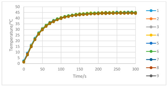
Figure 15.
Ten sets of temperature difference curves measured when the input current is 5 A.
Table 5.
Ten sets of and measured when the input current is 5 A.
It was assumed that the mean value of the ten sets of data was the actual value. The actual value can be obtained through as 0.1257. Each set of and measurements and was taken the mean between 200 s and 300 s. The ten sets of calibration tests obtained by Equation (8) found that the error of was between . In the main experiment, only the steady temperature difference needs to be measured. is a mean value between 200 s and 300 s in data processing, and the standard deviation was between 0.000427 and 0.00321. From , then the error expression is shown as:
Therefore, the error of the loss measurement experiment used in this paper was less than 10%. The temperatures were obtained by thermocouples and the temperature acquisition card. Under normal conditions, the influence of humidity and noise was negligible. The temperature isolation device can also avoid the influence of other heat sources of the system to a certain extent.
5. Conclusions
This paper analyzes in detail the principle of the temperature sensor measurement method and the advantages and disadvantages of various derivative methods. An optimized method is proposed: shorter time consuming, simpler measurement setup, and lower cost. Compared with the traditional methods, this method requires only one-eighth of the measurement time. Furthermore, only two thermocouples were especially necessary in this measurement, so it was easy to be applied in engineering. The loss measurement and error analysis were carried out in a three-level ANPC topology experiment platform based on the SiC&Si hybrid module. The accuracy and feasibility of this method were proven through a commonly-used electrical measurement. Through error analysis, we found that this method’s error was less than 10%.
Author Contributions
Conceptualization, X.Z., J.W. and Z.F.; data curation, S.Y.; formal analysis, Z.F. and J.W.; funding acquisition, X.Z. and J.W.; methodology, J.W.; resources, X.Z.; software, S.Y.; validation, Z.F.; writing, original draft, Z.F.; writing, review and editing, Z.F.
Funding
This paper is supported by the National Natural Science Foundation of China, Grant Number 51607053.
Conflicts of Interest
The authors declare no conflict of interest.
References
- Ma, J.; Lu, T.; He, F.; Wei, S.; Yuan, L.; Zhao, Z. Power loss analysis and optimization of three-level T-type converter based on hybrid devices. In Proceedings of the International Conference on Renewable Power Generation, Beijing, China, 17–18 October 2016; p. 6. [Google Scholar]
- Bilyi, D.; Gerling, D. Modeling of automotive power network for analysis of power electronics and losses calculation and verification by measurements on claw-pole alternator. In Proceedings of the IEEE International Power Electronics and Motion Control Conference, Hefei, China, 22–26 May 2016; pp. 3599–3605. [Google Scholar]
- Gottschlich, J.; Kaymak, M.; Christoph, M.; Doncker, R.W.D. A flexible test bench for power semiconductor switching loss measurements. In Proceedings of the IEEE International Conference on Power Electronics and Drive Systems, Sydney, NSW, Australia, 9–12 June 2015; pp. 442–448. [Google Scholar]
- Xiao, C.; Chen, G.; Odendaal, W.G. Overview of power loss measurement techniques in power electronics systems. IEEE Trans. Ind. Appl. 2007, 43, 657–664. [Google Scholar] [CrossRef]
- Jon, A.; Christoph, G.; Lukas, S.; Johann W., K. Accurate Calorimetric Switching Loss Measurement for 900 V 10 mΩ SiC MOSFETs. IEEE Trans. Power Electron. 2017, 32, 8963–8968. [Google Scholar]
- Tiwari, S.; Langelid, J.K.; Midtgård, O.M.; Undeland, T.M. Soft Switching Loss Measurements of a 1.2 kV SiC MOSFET Module by both Electrical and Calorimetric Methods for High Frequency Applications. In Proceedings of the 2017 19th European Conference on Power Electronics and Applications (EPE’17 ECCE Europe), Warsaw, Poland, 11–14 September 2017. [Google Scholar]
- Sverko, M.; Krishnamurthy, S. Calorimetric loss measurement system for air and water cooled power converters. In Proceedings of the 2013 15th European Conference on Power Electronics and Applications (EPE), Lille, France, 2–6 September 2013; pp. 1–10. [Google Scholar]
- Bortis, D.; Knecht, O.; Neumayr, D.; Kolar, J.W. Comprehensive evaluation of GaN GIT in low- and high-frequency bridge leg applications. In Proceedings of the IEEE International Power Electronics and Motion Control Conference, Hefei, China, 22–26 May 2016; pp. 21–30. [Google Scholar]
- Bolte, S.; Wohlrab, L.; Afridi, J.K.; Froehleke, N.; Boecker, J. Calorimetric Measurement of Wide Bandgap Semiconductors Switching Losses. In Proceedings of the PCIM Europe 2017, International Exhibition and Conference for Power Electronics, Intelligent Motion, Renewable Energy and Energy Management, Nuremberg, Germany, 16–18 May 2017. [Google Scholar]
- Bolte, S.; Fröhleke, N.; Böcker, J. DC-DC converter design for power distribution systems in electric vehicles using calorimetric loss measurements. In Proceedings of the European Conference on Power Electronics and Applications, Karlsruhe, Germany, 5–9 September 2016; pp. 1–7. [Google Scholar]
- Cao, W.; Huang, X.; French, I. Design of a 300-kW calorimeter for electrical motor loss measurement. IEEE Trans. Instrum. Meas. 2009, 58, 2365–2367. [Google Scholar]
- Wolfs, P.; Li, Q. Precision calorimetry for power loss measurement of a very low power maximum power point tracker. In Proceedings of the 2007 Australasian Universities Power Engineering Conference, Perth, WA, Australia, 9–12 December 2007. [Google Scholar]
- Simpson, N.; Hopkins, A.N. An accurate and flexible calorimeter topology for power electronic system loss measurement. In Proceedings of the 2017 IEEE International Electric Machines and Drives Conference (IEMDC), Miami, FL, USA, 21–24 May 2017. [Google Scholar]
- Chen, G.; Xiao, C.; Odendaal, W.G. An apparatus for loss measurement of integrated power electronics modules: design and analysis. In Proceedings of the Conference Record of the 2002 IEEE Industry Applications Conference. 37th IAS Annual Meeting (Cat. No.02CH37344), Pittsburgh, PA, USA, 13–18 October 2002; Volume 1, pp. 222–226. [Google Scholar]
- Pai, A.P.; Reiter, T.; Maerz, M. Mission profile analysis and calorimetric loss measurement of a SiC hybrid module for main inverter application of electric vehicles. In Proceedings of the 2017 IEEE International Workshop On Integrated Power Packaging (IWIPP), Delft, The Netherlands, 5–7 April 2017. [Google Scholar]
- Pai, A.P.; Reiter, T.; Vodyakho, O.; Yoo, I.; Maerz, M. A calorimetrie method for measuring power losses in power semiconductor modules. In Proceedings of the 2017 19th European Conference on Power Electronics and Applications (EPE’17 ECCE Europe), Warsaw, Poland, 11–14 September 2017. [Google Scholar]
- Anthon, A.; Zhang, Z.; Andersen, M.A.; Holmes, D.G.; McGrath, B.; Teixeira, C.A. The Benefits of SiC mosfet s in a T-Type Inverter for Grid-Tie Applications. IEEE Trans. Power Electron. 2017, 32, 2808–2821. [Google Scholar] [CrossRef]
- Rothmund, D.; Bortis, D.; Kolar, J.W. Accurate Transient Calorimetric Measurement of Soft-Switching Losses of 10kV SiC MOSFETs. In Proceedings of the 2016 IEEE 7th International Symposium on Power Electronics for Distributed Generation Systems (PEDG), Vancouver, BC, Canada, 27–30 June 2016. [Google Scholar]
- Li, H.; Li, X.; Zhang, Z.; Wang, J.; Liu, L.; Bala, S. A simple calorimetric technique for high-efficiency GaN inverter transistor loss measurement. In Proceedings of the 2017 IEEE 5th Workshop on Wide Bandgap Power Devices and Applications (WiPDA), Albuquerque, NM, USA, 30 October–1 November 2017. [Google Scholar]
- Hoffmann, L.; Gautier, C.; Lefebvre, S.; Costa, F. Optimization of the driver of GaN power transistors through measurement of their thermal behavior. IEEE Trans. Power Electron. 2014, 29, 2359–2366. [Google Scholar] [CrossRef]
- Neumayr, D.; Guacci, M.; Bortis, D.; Kolar, J.W. New calorimetric power transistor soft-switching loss measurement based on accurate temperature rise monitoring. In Proceedings of the 2017 29th International Symposium on Power Semiconductor Devices and IC’s (ISPSD), Sapporo, Japan, 28 May–1 June 2017. [Google Scholar]
- Zhang, Y.; Jahns, T.M. Power electronics loss measurement using new heat flux sensor based on thermoelectric device with active control. IEEE Trans. Ind. Appl. 2014, 50, 4098–4106. [Google Scholar] [CrossRef]
- Iero, D.; Della Corte, F.G.; Fiorentino, G.; Sarro, P.M. A calorimetry-based measurement apparatus for switching losses in high power electronic devices. In Proceedings of the 2016 IEEE International Energy Conference (ENERGYCON), Leuven, Belgium, 4–8 April 2016. [Google Scholar]
- Iero, D.; Della Corte, F.G.; Fiorentino, G.; Sarro, P.M.; Morana, B. A measurement apparatus for switching losses based on a heat-flux sensor. In Proceedings of the 2015 XVIII AISEM Annual Conference, Trento, Italy, 3–5 February 2015. [Google Scholar]
- Iero, D.; Della Corte, F.G.; Fiorentino, G.; Sarro, P.M.; Morana, B. Heat flux sensor for power loss measurements of switching devices. In Proceedings of the 19th International Workshop on Thermal Investigations of ICs and Systems (THERMINIC), Berlin, Germany, 25–27 September 2013. [Google Scholar]
- Schmid, H. Switching losses of the new SIRET-a comparison to other medium-power devices. In Proceedings of the Conference Record of the 1988 IEEE Industry Applications Society Annual Meeting, Pittsburgh, PA, USA, 2–7 October 1988. [Google Scholar]
- Marco Iachello, M.; Luca, V.D.; Petrone, G.; Testa, N.; Fortuna, L.; Cammarata, G.; Graziani, S.; Frasca, M. Lumped Parameter Modeling for Thermal Characterization of High-Power Modules. IEEE Trans. Compon. Packag. Manuf. Technol. 2014, 4, 1613–1623. [Google Scholar] [CrossRef]
- Famoso, C.; di Guardo, M.; Fortuna, L.; Frasca, M.; Graziani, S.; Testa, N. A system-of-systems based equipment for thermo-mechanical testing of advanced high power modules. In Proceedings of the 2015 IEEE International Symposium on Circuits and Systems (ISCAS), Lisbon, Portugal, 24–27 May 2015; pp. 197–200. [Google Scholar] [CrossRef]
- Floricau, D.; Floricau, E.; Gateau, G. Three-level active NPC converter: PWM strategies and loss distribution. In Proceedings of the 2008 34th Annual Conference of IEEE Industrial Electronics, Orlando, FL, USA, 10–13 November 2008. [Google Scholar]
© 2019 by the authors. Licensee MDPI, Basel, Switzerland. This article is an open access article distributed under the terms and conditions of the Creative Commons Attribution (CC BY) license (http://creativecommons.org/licenses/by/4.0/).