Figure 1.
Power losses qualification in electric network.
Figure 1.
Power losses qualification in electric network.
Figure 2.
The dependence of increasing active power losses (APL) from three-phase active power consumption for aluminium conductor steel reinforced (ACSR) 42/7 without consideration of voltage dip.
Figure 2.
The dependence of increasing active power losses (APL) from three-phase active power consumption for aluminium conductor steel reinforced (ACSR) 42/7 without consideration of voltage dip.
Figure 3.
The dependence of increasing APL from three-phase active power consumption for ACSR 70/11 without consideration of voltage dip.
Figure 3.
The dependence of increasing APL from three-phase active power consumption for ACSR 70/11 without consideration of voltage dip.
Figure 4.
The dependence of increasing APLs from three-phase active power consumption for ACSR 95/15 without consideration of voltage dip.
Figure 4.
The dependence of increasing APLs from three-phase active power consumption for ACSR 95/15 without consideration of voltage dip.
Figure 5.
The dependence of increasing APLs from three-phase active power consumption for ACSR 42/7 with consideration of voltage dip.
Figure 5.
The dependence of increasing APLs from three-phase active power consumption for ACSR 42/7 with consideration of voltage dip.
Figure 6.
The dependence of increasing APLs from three-phase active power consumption for ACSR 70/11 with consideration of voltage dip.
Figure 6.
The dependence of increasing APLs from three-phase active power consumption for ACSR 70/11 with consideration of voltage dip.
Figure 7.
The dependence of increasing APLs from three-phase active power consumption for ACSR 95/15 with consideration of voltage dip.
Figure 7.
The dependence of increasing APLs from three-phase active power consumption for ACSR 95/15 with consideration of voltage dip.
Figure 8.
Scenario 2: (a) ACSR 42/7; (b) ACSR 70/11.
Figure 8.
Scenario 2: (a) ACSR 42/7; (b) ACSR 70/11.
Figure 9.
Scenario 3: (a) ACSR 42/7; (b) ACSR 70/11.
Figure 9.
Scenario 3: (a) ACSR 42/7; (b) ACSR 70/11.
Figure 10.
Scenario 4: (a) ACSR 42/7; (b) ACSR 70/11.
Figure 10.
Scenario 4: (a) ACSR 42/7; (b) ACSR 70/11.
Figure 11.
Scenario 5: (a) ACSR 42/7; (b) ACSR 70/11.
Figure 11.
Scenario 5: (a) ACSR 42/7; (b) ACSR 70/11.
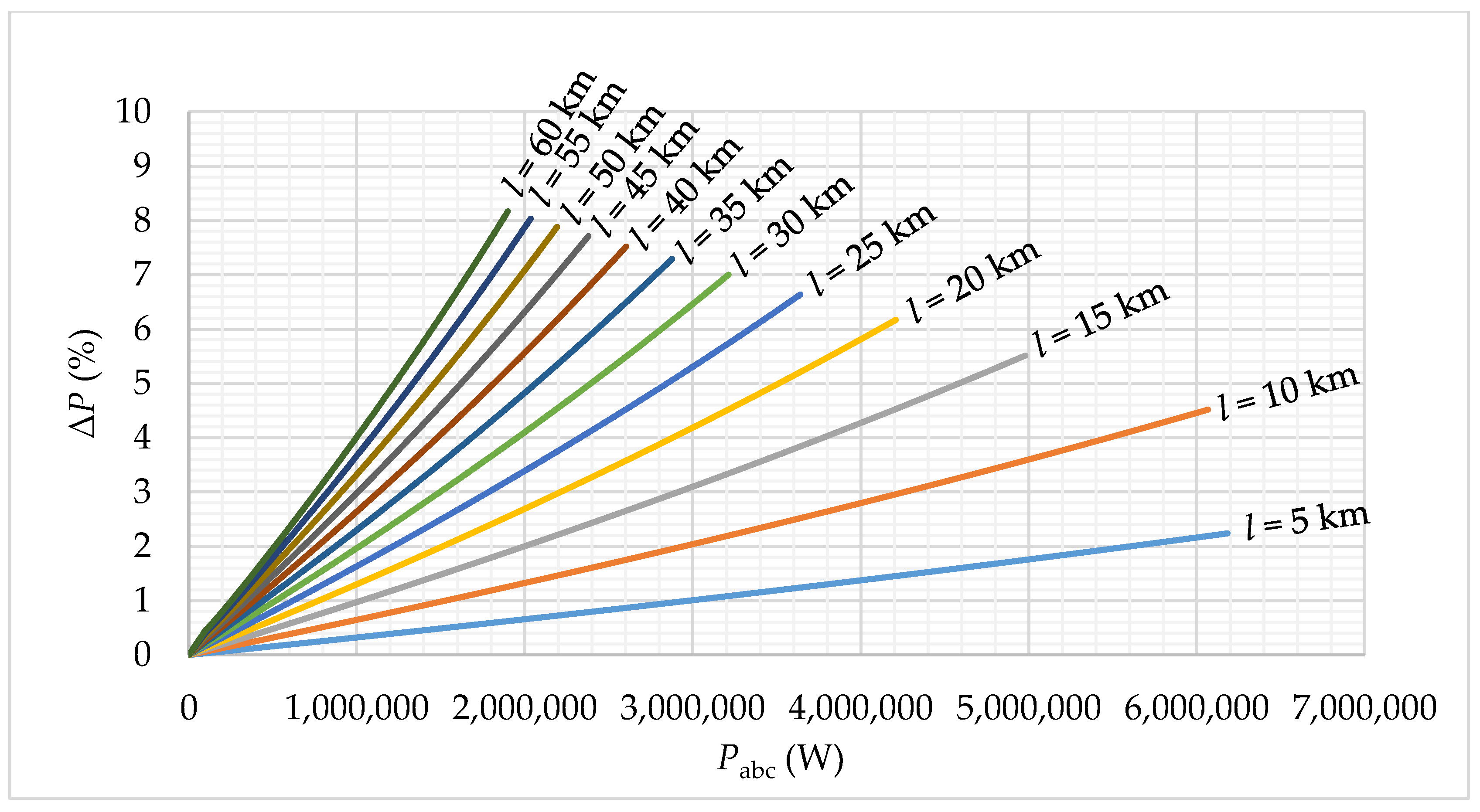
Figure 12.
The dependence of increasing APLs from three-phase active power consumption for ACSR 42/7: (a) the length of 5 km; (b) the length of 30 km.
Figure 12.
The dependence of increasing APLs from three-phase active power consumption for ACSR 42/7: (a) the length of 5 km; (b) the length of 30 km.
Figure 13.
The dependence of increasing APLs from three-phase active power consumption for ACSR 70/11: (a) the length of 5 km; (b) the length of 30 km.
Figure 13.
The dependence of increasing APLs from three-phase active power consumption for ACSR 70/11: (a) the length of 5 km; (b) the length of 30 km.
Figure 14.
The dependence of increasing APLs from three-phase active power consumption for ACSR 95/15: (a) the length of 5 km; (b) the length of 30 km.
Figure 14.
The dependence of increasing APLs from three-phase active power consumption for ACSR 95/15: (a) the length of 5 km; (b) the length of 30 km.
Figure 15.
The dependence of increasing APLs from three-phase active power consumption for ACSR 42/7: (a) the length of 5 km; (b) the length of 30 km.
Figure 15.
The dependence of increasing APLs from three-phase active power consumption for ACSR 42/7: (a) the length of 5 km; (b) the length of 30 km.
Figure 16.
The dependence of increasing APLs from three-phase active power consumption for ACSR 70/11: (a) the length of 5 km; (b) the length of 30 km.
Figure 16.
The dependence of increasing APLs from three-phase active power consumption for ACSR 70/11: (a) the length of 5 km; (b) the length of 30 km.
Figure 17.
The dependence of increasing APLs from three-phase active power consumption for ACSR 95/15: (a) the length of 5 km; (b) the length of 30 km.
Figure 17.
The dependence of increasing APLs from three-phase active power consumption for ACSR 95/15: (a) the length of 5 km; (b) the length of 30 km.
Figure 18.
Distribution grid for the analysis of the influence of individual factors.
Figure 18.
Distribution grid for the analysis of the influence of individual factors.
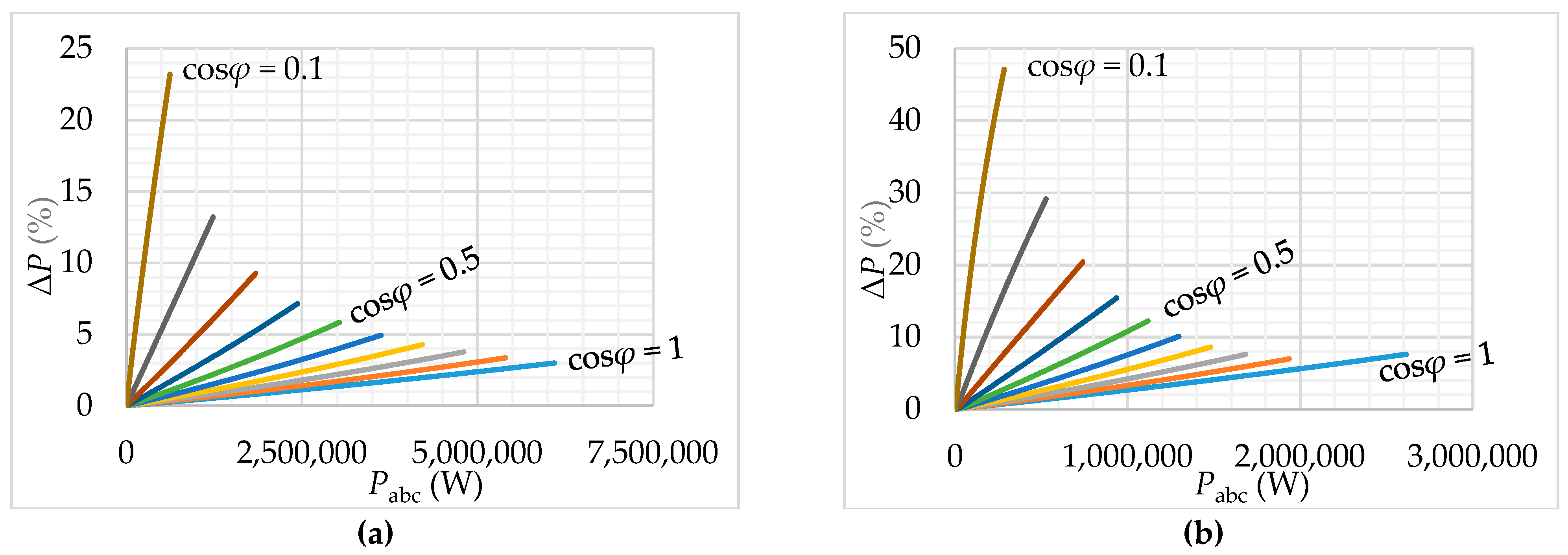
Figure 19.
The graphic dependence of increasing APLs from power factor (PF): (a) the length of 20 km; (b) the length of 40 km.
Figure 19.
The graphic dependence of increasing APLs from power factor (PF): (a) the length of 20 km; (b) the length of 40 km.
Figure 20.
The comparison of the APLs for three types of active power and three types of conductors.
Figure 20.
The comparison of the APLs for three types of active power and three types of conductors.
Figure 21.
The comparison of the APLs for three types of active powers for conductor ACSR 42/7.
Figure 21.
The comparison of the APLs for three types of active powers for conductor ACSR 42/7.
Figure 22.
The comparison of the APLs for three types of active powers for conductor ACSR 70/11.
Figure 22.
The comparison of the APLs for three types of active powers for conductor ACSR 70/11.
Figure 23.
The comparison of the APLs for three types of active powers for conductor ACSR 95/15.
Figure 23.
The comparison of the APLs for three types of active powers for conductor ACSR 95/15.
Figure 24.
The comparison of the APLs for three types of active powers for conductor ACSR 42/7.
Figure 24.
The comparison of the APLs for three types of active powers for conductor ACSR 42/7.
Figure 25.
The comparison of the APLs for three types of active powers for conductor ACSR 70/11.
Figure 25.
The comparison of the APLs for three types of active powers for conductor ACSR 70/11.
Figure 26.
The comparison of the APLs for three types of active powers for conductor ACSR 95/15.
Figure 26.
The comparison of the APLs for three types of active powers for conductor ACSR 95/15.
Figure 27.
The scheme of measured and modelled distribution grid.
Figure 27.
The scheme of measured and modelled distribution grid.
Figure 28.
The voltages (full line) and the currents (chain line): (a) the measurement; (b) the simulation.
Figure 28.
The voltages (full line) and the currents (chain line): (a) the measurement; (b) the simulation.
Figure 29.
The voltages (full line) and the currents (chain line): (a) the measurement; (b) the simulation.
Figure 29.
The voltages (full line) and the currents (chain line): (a) the measurement; (b) the simulation.
Figure 30.
The voltages (full line) and the currents (chain line): (a) the measurement; (b) the simulation.
Figure 30.
The voltages (full line) and the currents (chain line): (a) the measurement; (b) the simulation.
Figure 31.
The voltages (full line) and the currents (chain line): (a) the measurement; (b) the simulation.
Figure 31.
The voltages (full line) and the currents (chain line): (a) the measurement; (b) the simulation.
Figure 32.
Voltage levels at the measurement points in the distribution grid.
Figure 32.
Voltage levels at the measurement points in the distribution grid.
Figure 33.
Current levels at the measurement points in the distribution grid.
Figure 33.
Current levels at the measurement points in the distribution grid.
Figure 34.
Active power levels at the measurement points in the distribution grid.
Figure 34.
Active power levels at the measurement points in the distribution grid.
Figure 35.
Current harmonic spectrum at the measurement points.
Figure 35.
Current harmonic spectrum at the measurement points.
Figure 36.
Voltage harmonic spectrum at the measurement points.
Figure 36.
Voltage harmonic spectrum at the measurement points.
Table 1.
Rapid voltage change [
15].
Table 1.
Rapid voltage change [
15].
| Rapid Voltage Change | Max. Frequency for 24 h |
|---|
| ΔUSteady state ≥ 3 % | 24 |
| ΔUMax ≥ 5 % | 24 |
Table 2.
Parameters of flicker severity [
15].
Table 2.
Parameters of flicker severity [
15].
| Flicker Severity | 0.23 kV ≤ Un ≤ 35 kV | Time Period | Measurement |
|---|
| Short-term severity Pst (pu) | 1.2 | 95% of week | 10 min |
| Long-term severity Plt (pu) | 1.0 | 100% of time | 120 min |
Table 3.
Frequency of power supply in the Slovak Republic [
15].
Table 3.
Frequency of power supply in the Slovak Republic [
15].
| System | Mean Value of the Fundamental Frequency Measured over 10 s Intervals | Time |
|---|
| With the synchronous interconnection | 50 Hz ± 0.1 Hz (49.5 Hz…50.5 Hz) | 100% of the time |
| 50 Hz + 4%/−6% (47 Hz…52 Hz) | 100% of the time |
| Without the synchronous connection | 50 Hz ± 2% (49 Hz…51 Hz) | 100% of the time |
| 50 Hz ± 15% (42.5 Hz…57.5 Hz) | 100% of the time |
Table 4.
Three-phase values of active power and active power losses.
Table 4.
Three-phase values of active power and active power losses.
| Comparison | PABC (kW) | Pabc (kW) | ΔP (kW) | ΔP (%) |
|---|
| Measurement | 3866.00 | 3662.70 | 203.30 | 5.259 |
| Simulation | 3854.90 | 3660.39 | 194.51 | 5.046 |
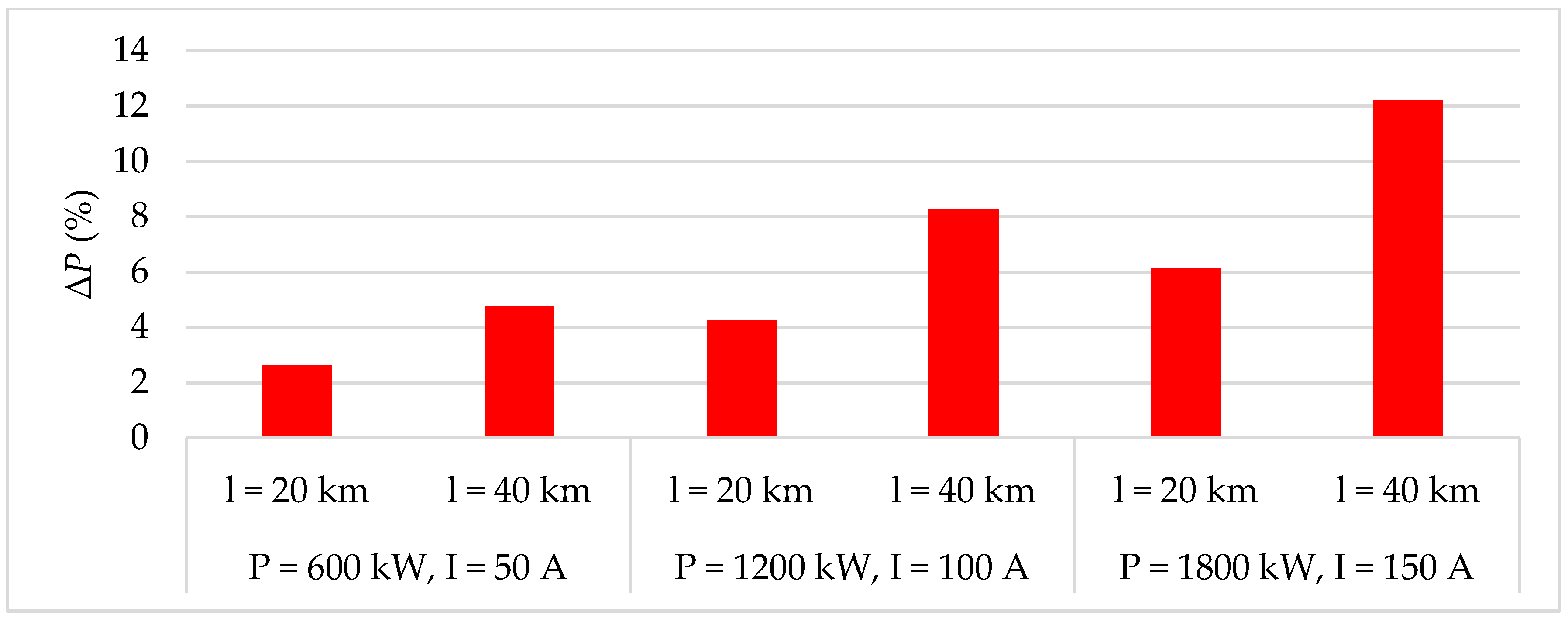
Table 5.
Overview of active power losses and their impact on finance (ACSR 70/11, length of 20 km).
Table 5.
Overview of active power losses and their impact on finance (ACSR 70/11, length of 20 km).
| Scenario | Load (kW) | Active Power Losses in MV Grid | Informative Price of Power Energy |
|---|
| ΔP (%) | ΔP (MW per hour) | ΔP (MW per year) | ΔPAdd (MW per year) | 40.00 EURO |
|---|
| Symmetric | 1233.7 | 2.586 | 0.0319 | 279.444 | 0 | 0.00 EURO |
| Unbalance 40:40:20 | 1235.3 | 2.752 | 0.0340 | 297.840 | 18.396 | 735.84 EURO |
| Unbalance 40:30:30 | 1233.8 | 2.650 | 0.0327 | 286.452 | 7.008 | 280.32 EURO |
| Unbalance 50:30:20 | 1236.3 | 2.831 | 0.0350 | 306.600 | 27.156 | 1086.24 EURO |
| Unbalance 50:40:10 | 1240.4 | 3.193 | 0.0396 | 346.896 | 67.452 | 2698.08 EURO |
| Unbalance 60:20:20 | 1242.5 | 3.348 | 0.0416 | 364.416 | 84.972 | 3398.88 EURO |
| cosφ = 0.8 | 1245.0 | 3.614 | 0.0450 | 394.200 | 114.756 | 4590.24 EURO |
| cosφ = 0.85 | 1242.0 | 3.382 | 0.0420 | 367.920 | 88.476 | 3539.04 EURO |
| cosφ = 0.9 | 1236.0 | 2.913 | 0.0360 | 315.360 | 35.916 | 1436.64 EURO |
| cosφ = 0.95 | 1233.0 | 2.676 | 0.0330 | 289.080 | 9.636 | 385.44 EURO |
| Harmonics | 1204.4 | 2.765 | 0.0333 | 291.708 | 12.264 | 490.56 EURO |
Table 6.
Overview of active power losses and their impact on finance (ACSR 70/11, length of 40 km).
Table 6.
Overview of active power losses and their impact on finance (ACSR 70/11, length of 40 km).
| Scenario | Load (kW) | Active Power Losses in MV Grid | Informative Price of Power Energy |
|---|
| ΔP (%) | ΔP (MW per hour) | ΔP (MW per year) | ΔP (%) | ΔP (MW per hour) |
|---|
| Symmetric | 1261.0 | 4.687 | 0.0591 | 517.716 | 0 | 0.00 EURO |
| Unbalance 40:40:20 | 1265.4 | 5.129 | 0.0649 | 568.524 | 50.808 | 2032.32 EURO |
| Unbalance 40:30:30 | 1261.4 | 4.765 | 0.0601 | 526.476 | 8.760 | 350.40 EURO |
| Unbalance 50:30:20 | 1273.0 | 5.625 | 0.0716 | 627.216 | 109.500 | 4380.00 EURO |
| Unbalance 50:40:10 | 1283.9 | 6.410 | 0.0823 | 720.948 | 203.232 | 8129.28 EURO |
| Unbalance 60:20:20 | 1289.1 | 6.997 | 0.0902 | 790.152 | 272.436 | 10,897.44 EURO |
| cosφ = 0.8 | 1299.0 | 7.621 | 0.0990 | 867.240 | 349.524 | 13,980.96 EURO |
| cosφ = 0.85 | 1287.0 | 6.760 | 0.0870 | 762.120 | 244.404 | 9776.16 EURO |
| cosφ = 0.9 | 1275.0 | 5.882 | 0.0750 | 657.000 | 139.284 | 5571.36 EURO |
| cosφ = 0.95 | 1266.0 | 5.231 | 0.0660 | 578.160 | 60.444 | 2417.76 EURO |
| Harmonics | 1211.4 | 5.275 | 0.0639 | 559.764 | 42.048 | 1681.92 EURO |


