Fractional Order Fuzzy PID Control of Automotive PEM Fuel Cell Air Feed System Using Neural Network Optimization Algorithm

Abstract
:1. Introduction
- A new application for the FOFPID and FOPID controllers is proposed to apply in the PEMFC air feed control to improve performance and robustness.
- This paper employs a direct discretization approach using an Al-Alawi operator for the first time to implement fractional order fuzzy PID controllers rather than indirect discretization approach based on Oustaloup’s recursive approximation.
- This paper is the first application of the NNA algorithm in controller design applications.
- The proposed NNA optimized FOFPID controller is tested for a constant set value for the oxygen excess ratio as well as the maximum power point operation by tracking a time varying set value for the oxygen excess ratio.
- Sensitivity analyses are performed to test the robustness of the proposed controller under various uncertainty conditions.
2. PEMFC Model
2.1. Air Feed System Model for PEMFC
2.2. Control Objective
3. Air Feeding System Controller Design
3.1. Fractional-Order Operators and Its Discretization
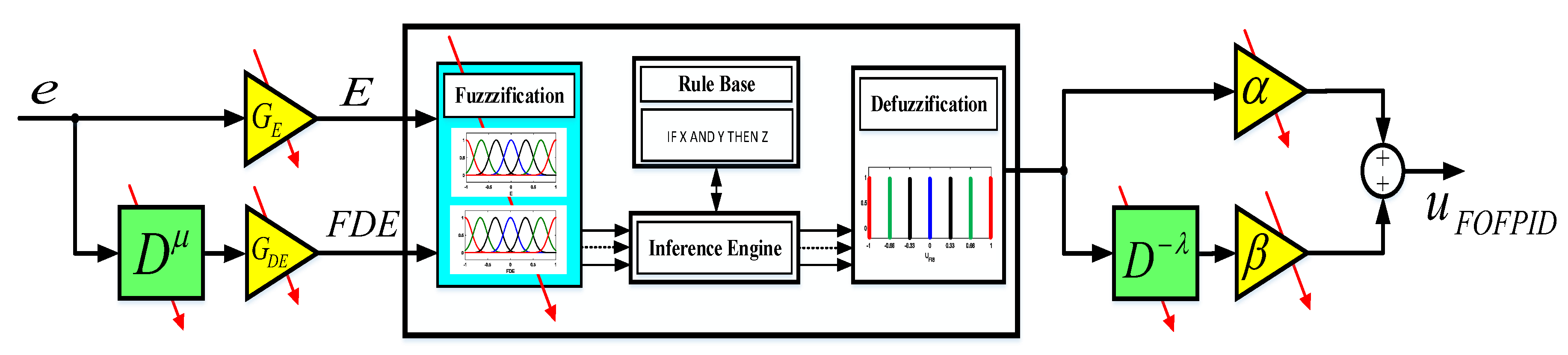
3.2. Fractional Order Fuzzy PID Controller
4. Optimization Tool
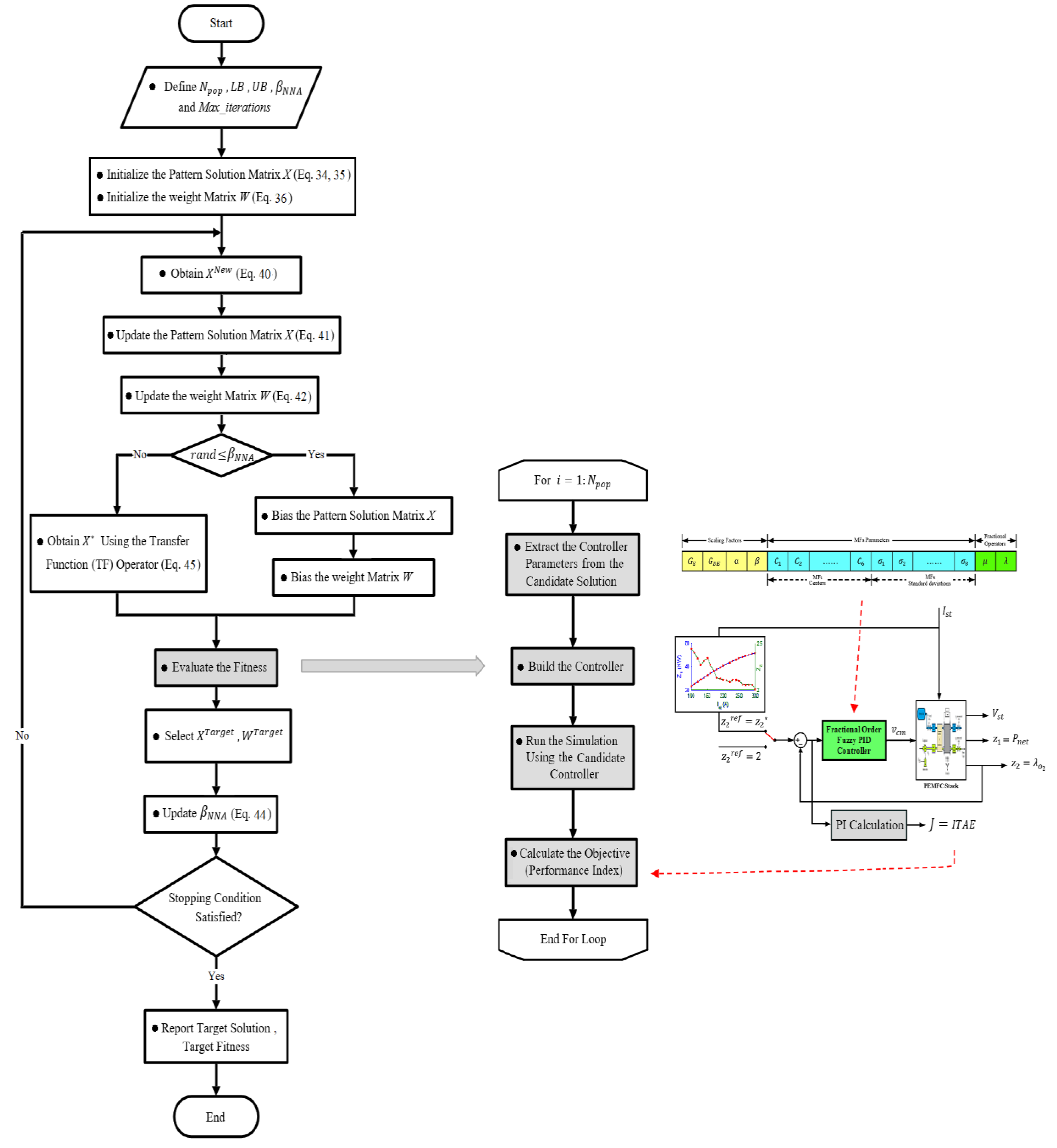
4.1. Neural Network Algorithm (NNA)
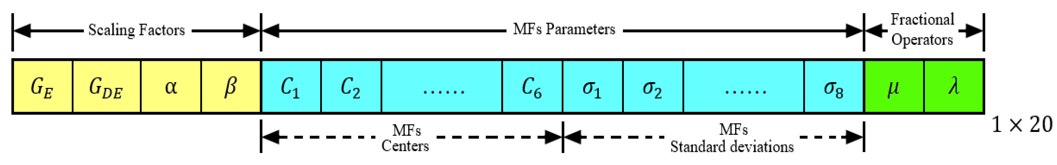
4.2. Formulation of FOFPID Controller Design as an Optimization Problem
5. Simulation Results and Discussion
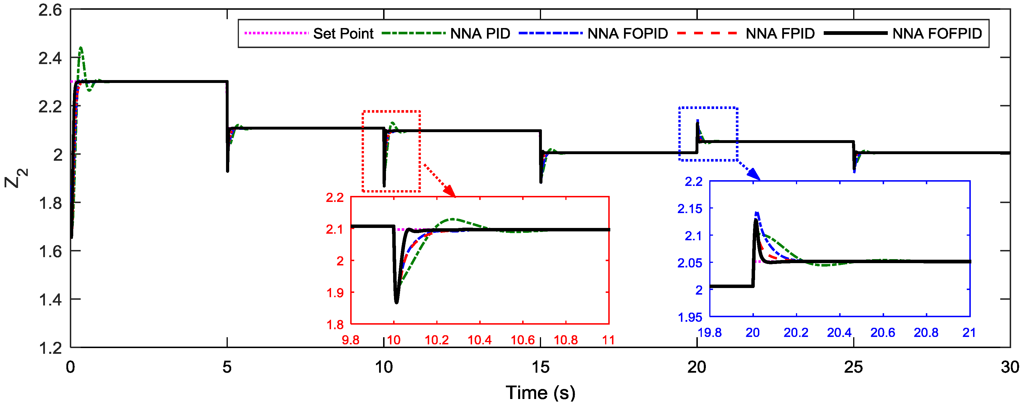
5.1. The First Task (Tracking Constant )
5.2. The Second Task (MPPT)
5.3. The Third Task (Sensitivity Analysis)
6. Conclusions
Author Contributions
Funding
Acknowledgments
Conflicts of Interest
Appendix A

| Fuel Cells (FC) Data | |||
| Number of cells in fuel cell stack | 381 | ||
| The volume of the cathode | 0.01 | ||
| Throttle discharge coefficient for the cathode outlet | 0.0124 | ||
| Cathode outlet throttle area | 0.00175 | ||
| Supply manifold volume | 0.02 | ||
| Fuel cell temperature | 353.15 | ||
| Cathode inlet orifice constant | 0.3629 × | ||
| Air & Steam Properties | |||
| Ratio of specific heats of air | 1.4 | ||
| Nitrogen molar mass | 28 × | ||
| Oxygen molar mass | 32 × | ||
| Vapor molar mass | 18.02 × | ||
| Air molar mass | 28.97 × | ||
| Atmospheric temperature | 298.15 | ||
| Atmospheric pressure | 1.01325 × | ||
| Specific heat of air at constant pressure | 1004 | ||
| Average relative humidity of the ambient air | 0.5 | ||
| Oxygen mole fraction | 0.21 | ||
| Electrochemistry | |||
| Faraday constant | 96.487 | ||
| Universal gas constant | 8.31451 | ||
| Compressor (CP) | |||
| Compressor efficiency | 80% | ||
| Compressor inertia | 5 × | ||
| Compressor Motor (CM) | |||
| Compressor motor resistance | 0.82 | ||
| Motor constant | 0.0225 | ||
| Motor constant | 0.0153 | ||
| Motor mechanical efficiency | 98% | ||
References
- Pathapati, P.R.; Xue, X.; Tang, J. A new dynamic model for predicting transient phenomena in a PEM fuel cell system. Renew. Energy 2005, 30, 1–22. [Google Scholar] [CrossRef]
- Liu, J.; Gao, Y.; Su, X.; Wack, M.; Wu, L. Disturbance-observer-based control for air management of PEM fuel cell systems via sliding mode technique. IEEE Trans. Control Syst. Technol. 2018, 99, 1–10. [Google Scholar] [CrossRef]
- Vahidi, A.; Stefanopoulou, A.; Peng, H. Current management in a hybrid fuel cell power system: A model-predictive control approach. IEEE Trans. Control Syst. Technol. 2006, 14, 1047–1057. [Google Scholar] [CrossRef]
- Pukrushpan, J.T.; Peng, H.; Stefanopoulou, A.G. Control-Oriented Modeling and Analysis for Automotive Fuel Cell Systems. J. Dyn. Syst. Meas. Control 2004, 126, 14–25. [Google Scholar] [CrossRef]
- Pukrushpan, J.T.; Stefanopoulou, A.G.; Huei, P. Modeling and Control for PEM Fuel Cell Stack System. In Proceedings of the American Control Conference, Anchorage, AK, USA, 8–10 May 2002; Volume 4, pp. 3117–3122. [Google Scholar]
- Pukrushpan, J.T.; Stefanopoulou, A.G.; Huei, P. Control of fuel cell breathing. IEEE Control Syst. 2004, 24, 30–46. [Google Scholar]
- Grujicic, M.; Chittajallu, K.M.; Law, E.H.; Pukrushpan, J.T. Model-based control strategies in the dynamic interaction of air supply and fuel cell. Proc. Inst. Mech. Eng. Part A J. Power Energy 2004, 218, 487–499. [Google Scholar] [CrossRef]
- Niknezhadi, A.; Allué-Fantova, M.; Kunusch, C.; Ocampo-Martínez, C. Design and implementation of LQR/LQG strategies for oxygen stoichiometry control in PEM fuel cells based systems. J. Power Sour. 2011, 196, 4277–4282. [Google Scholar] [CrossRef] [Green Version]
- Talj, R.; Hilairet, M.; Ortega, R. Second order sliding mode control of the moto-compressor of a PEM fuel cell air feeding system, with experimental validation. In Proceedings of the 35th Annual Conference of IEEE Industrial Electronics, Porto, Portugal, 3–5 November 2009; pp. 2790–2795. [Google Scholar]
- Laghrouche, S.; Liu, J.; Ahmed, F.S.; Harmouche, M.; Wack, M. Adaptive second-order sliding mode observer-based fault reconstruction for PEM fuel cell air-feed system. IEEE Trans. Control Syst. Technol. 2015, 23, 1098–1109. [Google Scholar] [CrossRef]
- Han, J.; Yu, S.; Yi, S. Adaptive control for robust air flow management in an automotive fuel cell system. Appl. Energy 2017, 190, 73–83. [Google Scholar] [CrossRef]
- Gruber, J.K.; Doll, M.; Bordons, C. Design and experimental validation of a constrained MPC for the air feed of a fuel cell. Control Eng. Pract. 2009, 17, 874–885. [Google Scholar] [CrossRef]
- Wang, Y.-X.; Xuan, D.-J.; Kim, Y.-B. Design and experimental implementation of time delay control for air supply in a polymer electrolyte membrane fuel cell system. Int. J. Hydrogen Energy 2013, 38, 13381–13392. [Google Scholar] [CrossRef]
- Sanchez, V.M.; Barbosa, R.; Arriaga, L.G.; Ramirez, J.M. Real time control of air feed system in a PEM fuel cell by means of an adaptive neural-network. Int. J. Hydrogen Energy 2014, 39, 16750–16762. [Google Scholar] [CrossRef]
- Beirami, H.; Shabestari, A.Z.; Zerafat, M.M. Optimal PID plus fuzzy controller design for a PEM fuel cell air feed system using the self-adaptive differential evolution algorithm. Int. J. Hydrogen Energy 2015, 40, 9422–9434. [Google Scholar] [CrossRef]
- Baroud, Z.; Benmiloud, M.; Benalia, A.; Ocampo-Martinez, C. Novel hybrid fuzzy-PID control scheme for air supply in PEM fuel-cell-based systems. Int. J. Hydrogen Energy 2017, 42, 10435–10447. [Google Scholar] [CrossRef] [Green Version]
- Robles Algarín, C.; Taborda Giraldo, J.; Rodríguez Álvarez, O. Fuzzy logic based MPPT controller for a PV system. Energies 2017, 10, 2036. [Google Scholar] [CrossRef]
- Sahu, B.K.; Pati, S.; Mohanty, P.K.; Panda, S. Teaching–learning based optimization algorithm based fuzzy-PID controller for automatic generation control of multi-area power system. Appl. Soft Comput. 2015, 27, 240–249. [Google Scholar] [CrossRef]
- Omar, M.S.A.; Khedr, T.Y.; Zalam, B.A.A. Particle swarm optimization of fuzzy supervisory controller for nonlinear position control system. In Proceedings of the 8th International Conference on Computer Engineering & Systems (ICCES), Cairo, Egypt, 26–28 November 2013; pp. 138–145. [Google Scholar]
- Podlubny, I. Fractional-order systems and PIλDμ controller. IEEE Trans. Autom. Control 1999, 44, 208–214. [Google Scholar] [CrossRef]
- Alomoush, M.I. Load frequency control and automatic generation control using fractional-order controllers. Electr. Eng. 2010, 91, 357–368. [Google Scholar] [CrossRef]
- Debbarma, S.; Saikia, L.C.; Sinha, N. AGC of a multi-area thermal system under deregulated environment using a non-integer controller. Electr. Power Syst. Res. 2013, 95, 175–183. [Google Scholar] [CrossRef]
- Sondhi, S.; Hote, Y.V. Management, Fractional order PID controller for load frequency control. Energy Convers. 2014, 85, 343–353. [Google Scholar] [CrossRef]
- Taher, S.A.; Fini, M.H.; Aliabadi, S.F. Fractional order PID controller design for LFC in electric power systems using imperialist competitive algorithm. Ain Shams Eng. J. 2014, 5, 121–135. [Google Scholar] [CrossRef] [Green Version]
- Pan, I.; Das, S. Fractional-order load-frequency control of interconnected power systems using chaotic multi-objective optimization. Appl. Soft Comput. 2015, 29, 328–344. [Google Scholar] [CrossRef] [Green Version]
- Das, S.; Pan, I.; Das, S.; Gupta, A. A novel fractional order fuzzy PID controller and its optimal time domain tuning based on integral performance indices. Eng. Appl. Artif. Intell. 2012, 25, 430–442. [Google Scholar] [CrossRef] [Green Version]
- Pan, I.; Das, S. Fractional order fuzzy control of hybrid power system with renewable generation using chaotic PSO. ISA Trans. 2016, 62, 19–29. [Google Scholar] [CrossRef] [PubMed] [Green Version]
- Kumar, A.; Kumar, V. Communications, Hybridized ABC-GA optimized fractional order fuzzy pre-compensated FOPID control design for 2-DOF robot manipulator. AEU Int. J. Electron. 2017, 79, 219–233. [Google Scholar] [CrossRef]
- Mahto, T.; Mukherjee, V. Distribution, Fractional order fuzzy PID controller for wind energy-based hybrid power system using quasi-oppositional harmony search algorithm. IET Gener. Transm. 2017, 11, 3299–3309. [Google Scholar] [CrossRef]
- Arya, Y.; Kumar, N. BFOA-scaled fractional order fuzzy PID controller applied to AGC of multi-area multi-source electric power generating systems. Swarm Evol. Comput. 2017, 32, 202–218. [Google Scholar] [CrossRef]
- Sadollah, A.; Sayyaadi, H.; Yadav, A. A dynamic metaheuristic optimization model inspired by biological nervous systems: Neural network algorithm. Appl. Soft Comput. 2018, 71, 747–782. [Google Scholar] [CrossRef]
- Pukrushpan, J.T. Modeling and Control of Fuel Cell Systems and Fuel Processors; University of Michigan: Ann Arbor, MI, USA, 2003. [Google Scholar]
- Suh, K.W. Modeling, analysis and control of fuel cell hybrid power systems. Ph.D. Thesis, University of Michigan, Ann Arbor, MI, USA, January 2006. [Google Scholar]
- Deng, H.; Li, Q.; Cui, Y.; Zhu, Y.; Chen, W. Nonlinear controller design based on cascade adaptive sliding mode control for PEM fuel cell air supply systems. Int. J. Hydrogen Energy 2018. [Google Scholar] [CrossRef]
- Gruber, J.K.; Bordons, C.; Dorado, F. Nonlinear control of the air feed of a fuel cell. In Proceedings of the American Control Conference, Seattle, WA, USA, 11–13 June 2008; pp. 1121–1126. [Google Scholar]
- Talj, R.J.; Hissel, D.; Ortega, R.; Becherif, M.; Hilairet, M. Experimental Validation of a PEM Fuel-Cell Reduced-Order Model and a Moto-Compressor Higher Order Sliding-Mode Control. IEEE Trans. Ind. Electron. 2010, 57, 1906–1913. [Google Scholar] [CrossRef]
- Talj, R.; Ortega, R.; Hilairet, M. A controller tuning methodology for the air supply system of a PEM fuel-cell system with guaranteed stability properties. Int. J. Control 2009, 82, 1706–1719. [Google Scholar] [CrossRef]
- Liu, J.; Gao, Y.; Geng, S.; Wu, L. Nonlinear control of variable speed wind turbines via fuzzy techniques. IEEE Access 2017, 5, 27–34. [Google Scholar] [CrossRef]
- Chen, Y.; Vinagre, B.M.; Podlubny, I. Continued fraction expansion approaches to discretizing fractional order derivatives—An expository review. Nonlinear Dyn. 2004, 38, 155–170. [Google Scholar] [CrossRef]
- Chen, Y.Q.; Moore, K.L. Discretization schemes for fractional-order differentiators and integrators. IEEE Trans. Circuits Syst. Fundam. Theory Appl. 2002, 49, 363–367. [Google Scholar] [CrossRef] [Green Version]
- Petrás, I. Fractional derivatives, fractional integrals, and fractional differential equations in Matlab. In Engineering Education and Research Using MATLAB; InTech: London, UK, 2011. [Google Scholar]
- Cheng, Y.-S.; Liu, Y.-H.; Hesse, H.; Naumann, M.; Truong, C.; Jossen, A. A PSO-Optimized Fuzzy Logic Control-Based Charging Method for Individual Household Battery Storage Systems within a Community. Energies 2018, 11, 469. [Google Scholar] [CrossRef]
- Sharma, R.; Rana, K.; Kumar, V. Performance analysis of fractional order fuzzy PID controllers applied to a robotic manipulator. Expert Syst. Appl. 2014, 41, 4274–4289. [Google Scholar] [CrossRef]


| PEMFC Model Constants | |
|---|---|
| NB | NM | NS | Z | PS | PM | PB | ||
|---|---|---|---|---|---|---|---|---|
| NB | NB | NB | NB | NB | NM | NS | Z | |
| NM | NB | NB | NB | NM | NS | Z | PS | |
| NS | NB | NB | NM | NS | Z | PS | PM | |
| Z | NB | NM | NS | Z | PS | PM | PB | |
| PS | NM | NS | Z | PS | PM | PB | PB | |
| PM | NS | Z | PS | PM | PB | PB | PB | |
| PB | Z | PS | PM | PB | PB | PB | PB | |
| Controller | ISE | IAE | ITSE | ITAE |
|---|---|---|---|---|
| PID [16] | 0.0627 | 0.2903 | NA | 2.2741 |
| FLC [16] | 0.5045 | 1.1047 | NA | 8.0201 |
| HFPID [16] | 0.0249 | 0.1005 | NA | 0.6781 |
| NNA PID | 0.03711 | 0.1995 | 0.1032 | 1.356 |
| NNA FOPID | 0.02652 | 0.1261 | 0.07036 | 0.8443 |
| NNA FPID | 0.014 | 0.09013 | 0.06015 | 0.6539 |
| NNA FOFPID (proposed) | 0.009186 | 0.05291 | 0.04193 | 0.3639 |
| Controller | ISE | IAE | ITSE | ITAE |
|---|---|---|---|---|
| HFPID [16] | NA | NA | NA | NA |
| NNA PID | 0.04931 | 0.1938 | 0.062 | 1.034 |
| NNA FOPID | 0.03104 | 0.1238 | 0.04675 | 0.7024 |
| NNA FPID | 0.03671 | 0.1127 | 0.03346 | 0.4368 |
| NNA FOFPID (proposed) | 0.02459 | 0.0701 | 0.02513 | 0.2619 |
| Parameter | % Change | ISE | IAE | ITSE | ITAE |
|---|---|---|---|---|---|
| Nominal | 0 | 0.02459 | 0.0701 | 0.02513 | 0.2619 |
| +25% | 0.0239 | 0.07184 | 0.03055 | 0.3069 | |
| −25% | 0.0263 | 0.07017 | 0.01969 | 0.2255 | |
| +25% | 0.0256 | 0.07463 | 0.03141 | 0.3158 | |
| −25% | 0.0239 | 0.06669 | 0.01997 | 0.225 | |
| +25% | 0.03594 | 0.08698 | 0.03287 | 0.3187 | |
| −25% | 0.01389 | 0.05485 | 0.01815 | 0.2263 | |
| +25% | 0.02459 | 0.0701 | 0.02513 | 0.2619 | |
| −25% | 0.02459 | 0.0701 | 0.02513 | 0.2619 | |
| +25% | 0.03929 | 0.1005 | 0.04467 | 0.519 | |
| −25% | 0.01774 | 0.05987 | 0.02576 | 0.2671 | |
| +25% | 0.0313 | 0.07813 | 0.02625 | 0.2707 | |
| −25% | 0.01966 | 0.06367 | 0.02441 | 0.2571 |
© 2019 by the authors. Licensee MDPI, Basel, Switzerland. This article is an open access article distributed under the terms and conditions of the Creative Commons Attribution (CC BY) license (http://creativecommons.org/licenses/by/4.0/).
Share and Cite
AbouOmar, M.S.; Zhang, H.-J.; Su, Y.-X. Fractional Order Fuzzy PID Control of Automotive PEM Fuel Cell Air Feed System Using Neural Network Optimization Algorithm. Energies 2019, 12, 1435. https://doi.org/10.3390/en12081435
AbouOmar MS, Zhang H-J, Su Y-X. Fractional Order Fuzzy PID Control of Automotive PEM Fuel Cell Air Feed System Using Neural Network Optimization Algorithm. Energies. 2019; 12(8):1435. https://doi.org/10.3390/en12081435
Chicago/Turabian StyleAbouOmar, Mahmoud S., Hua-Jun Zhang, and Yi-Xin Su. 2019. "Fractional Order Fuzzy PID Control of Automotive PEM Fuel Cell Air Feed System Using Neural Network Optimization Algorithm" Energies 12, no. 8: 1435. https://doi.org/10.3390/en12081435
APA StyleAbouOmar, M. S., Zhang, H.-J., & Su, Y.-X. (2019). Fractional Order Fuzzy PID Control of Automotive PEM Fuel Cell Air Feed System Using Neural Network Optimization Algorithm. Energies, 12(8), 1435. https://doi.org/10.3390/en12081435