Multi-Functional Model Predictive Control with Mutual Influence Elimination for Three-Phase AC/DC Converters in Energy Conversion

Abstract

Conventional model predictive control (MPC)-based direct power control of the three-phase full-bridge AC/DC converter usually suffers from the parametric coupling between active and reactive powers. A reference change of either the active or reactive power will influence the other, deteriorating the dynamic-state performance. In addition, the steady-state performance affected by one-step-delay arising from computation and communication processes in the digital implementation should be improved in consideration of switching frequency reduction. In combination with the proposed novel mutual influence elimination constraint, this paper proposes the multi-functional MPC for three-phase full-bridge AC/DC converters to improve both the steady and dynamic performances simultaneously. It has various advantages such as one-step-delay compensation, power ripple reduction, and switching frequency reduction for steady-state performance as well as mutual influence elimination for dynamic capability. The simulation and experimental results are obtained to verify the effectiveness of the proposed method.

1. Introduction

Nowadays, renewable energy sources are important to meet the growing energy demand and reduce reliance on fossil fuels [1]. The three-phase full-bridge converter is a popular option for integration of renewable energy sources [2], active power filters, electric drives and energy storage system (ESS) due to its merits such as four-quadrant power flow, natural power factor amendment, flexible DC-link voltage control, and low DC filter capacitance in comparison with the uncontrolled AC/DC converters [3,4,5]. Also, the fast development of renewable energy systems leads to more stringent requirements of advanced control strategies that can deliver better system reliability and power quality [6].

The direct power control (DPC) and voltage-oriented control (VOC) are typical control strategies [7,8,9,10,11,12]. The VOC controls the input powers by regulating the input current. Although the strategy has a good dynamics response and stability in steady-state, the inner current controller has a large impact on the whole system [13]. The DPC derives from the direct torque control in electric drives. It controls the powers directly through the selection of a suitable voltage vector from the preset switching table based on the instantaneous errors between the reference and instantaneous values of powers, and the space voltage vector location [14]. The DPC has a simple control algorithm and does not need an internal controller, but the control accuracy cannot be guaranteed.

The model predictive control (MPC) for power electronics applications and renewable energy systems has attracted lots of attention in recent years [15,16,17,18,19,20,21,22,23,24,25,26,27,28]. It is a flexible control method that enables simple addition of system nonlinearities and various constraints. In the MPC-based DPC scheme, system model and the cost function of errors between reference and measured powers are compared among each voltage vector, and the voltage vector that minimizes the cost function value is chosen for execution [29,30,31,32,33]. This approach is more accurate compared with DPC control and the control objectives can vary relatively according to the various cost function. In terms of conventional MPC-based DPC control, active and reactive powers could only be simultaneously controlled with a single cost function, and it has one-step-delay influence arising from computation and communication processes in the digital implementation [34]. The improved MPC was proposed to compensate the one-step-delay while reducing average switching frequency and keeping system stability [35]. This approach, however, only considers the system steady-state performance. During the transient state, if one control objective experiences a large change of the power reference value, relatively more weight is put on the changed objective due to parametric coupling. Then the voltage vector that is more likely to adjust this objective to the reference value would be selected according to the cost function. This influences the performance of the other control target since these two control objectives could not be completely decoupled according to the converter model and conventional cost function, which deteriorates the dynamic performance of active and reactive power control, and also causes the distortion of the output voltage waveform, especially when using the cost function consisting of square terms [36,37].

This mutual influence issue exists widely in most MPC-based methods no matter whether for multi-vector based control or for different control targets such as electrical machines, and the issue is more likely to occur in systems with a severe change of control objectives. This may impose more stress on the load system and decrease efficiency and operation performance of the system [38]. A modulated MPC scheme with vector duty cycle calculation was proposed in [38] to eliminate it. However, the proposed method is not a general constraint for model predictive based control and the steady-state performance issue was not considered.

In order to solve the aforementioned issues comprehensively, a general mutual influence elimination for MPC-based control has been proposed, also this paper proposes the multi-functional MPC to improve both the dynamic and steady-state performances simultaneously. Not only the novel control strategy can improve the steady-state performance by one-step-delay compensation, while improving the corresponding system deterioration issue such as switching frequency increment, but also improve the dynamic-state performance through eliminating the coupling between the active and reactive power control.

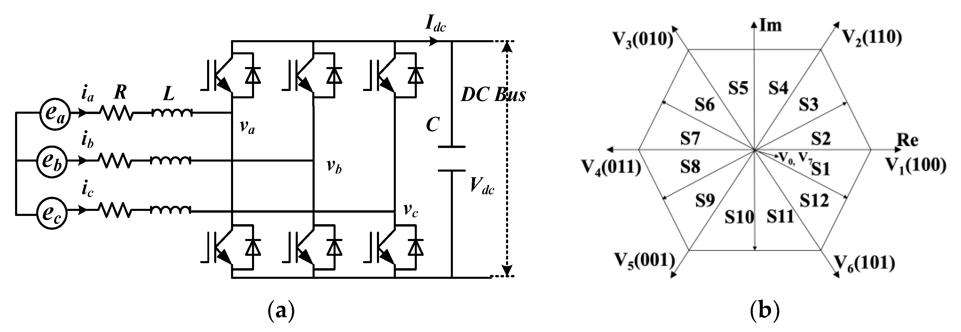
2. Modeling of Three-phase Full-bridge Converter

Figure 1a illustrates the topology of the three-phase full-bridge AC/DC converter that can be operated for bi-directional power conversion. The three-phase full-bridge unit is connected to the AC side via three inductors L and resistors R. At the DC side, a DC load or DC bus is connected to the bridge with a capacitor C in parallel connection, where e_a, e_b, and e_c are the three-phase AC source voltages; V_a, V_b, and V_c the AC terminal voltages of the three-phase bridge; and I_a, I_b, and I_c the three-phase currents. Figure 1b shows the voltage space vectors.

In the αβ-coordinate system, the AC source voltage vector and the current vector can be derived as:

$$e_{\alpha \beta }=\left[\begin{array}{c}{e}_{\alpha }\\ e_{\beta }\end{array}\right]=\frac{2}{3}\left[\begin{array}{ccc}1& -1/2& -1/2\\ 0& \sqrt{3}/2& -\sqrt{3}/2\end{array}\right]\left[\begin{array}{c}{e}_a\\ e_b\\ e_c\end{array}\right]$$

(1)

$$I_{\alpha \beta }=\left[\begin{array}{c}{I}_{\alpha }\\ I_{\beta }\end{array}\right]=\frac{2}{3}\left[\begin{array}{ccc}1& -1/2& -1/2\\ 0& \sqrt{3}/2& -\sqrt{3}/2\end{array}\right]\left[\begin{array}{c}{I}_a\\ I_b\\ I_c\end{array}\right]$$

(2)

In a balanced three-phase system, the line currents can be derived as below:

$$e_{\alpha \beta }=L\frac{d{I}_{a\beta }}{dt}+R{I}_{a\beta }+V_{\alpha \beta }$$

(3)

$$C\frac{d{V}_{dc}}{dt}=\frac{3}{2}\left(I_{\alpha }{S}_{\alpha }+I_{\beta }{S}_{\beta }\right)-I_L$$

(4)

where e_αβ, V_αβ, I_αβ, and I_L are the source voltage vector, the three-phase converter input voltage vector, the line current vector, and the load current, respectively, S_α and S_β are the switching switch states (0 = off, 1 = on), which are derived from switching state of each leg. The exchange between active and reactive power within the grid is derived as:

$$\left[\begin{array}{c}P\\ Q\end{array}\right]=\frac{3}{2}\left[\begin{array}{cc}{e}_{\alpha }& e_{\beta }\\ e_{\beta }& -e_{\alpha }\end{array}\right]\left[\begin{array}{c}{I}_{\alpha }\\ I_{\beta }\end{array}\right]$$

(5)

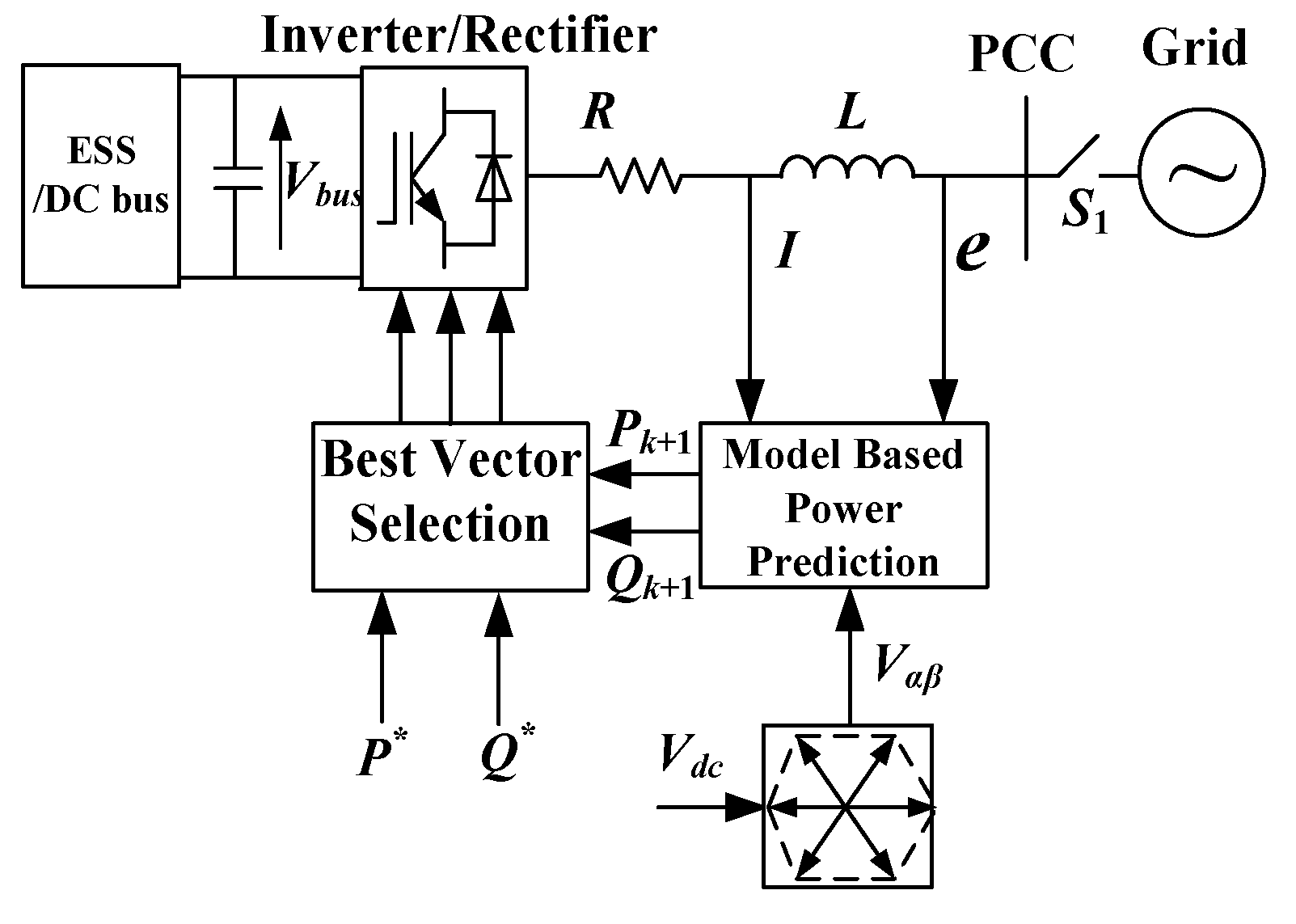
3. Predictive Model of AC/DC Converter

The conventional DPC (CDPC) is designed according to the instantaneous active and reactive powers to form the control loops, as described in [8]. The voltage vector of the PWM rectifier is chosen from a preset switching table. The switching table is formulated based on the power source voltage vector position, θ_n, in the α–β plane and the digitized signals S_p and S_q, where S_p and S_q are generated according to a fixed band hysteresis comparators and the tracking errors of active and reactive powers, respectively, S_p and S_q usually use indicators “0” and “1” to indicate two different status. More details regarding the control algorithm of CDPC can refer to [8].

The MPC-based DPC predicts the change of power at the time instant (k + 1) for different voltage vectors and applies the voltage vector that minimizes the cost function. Figure 2 shows the block diagram of MPC. The differential equation of active and reactive power can be derived from (5) as

$$\frac{d}{dt}\left[\begin{array}{c}P\\ Q\end{array}\right]=\frac{3}{2}\left(I_{\alpha }\frac{d}{dt}\left[\begin{array}{c}{e}_{\alpha }\\ e_{\beta }\end{array}\right]+\frac{d{I}_{\alpha }}{dt}\left[\begin{array}{c}{e}_{\alpha }\\ e_{\beta }\end{array}\right]+I_{\beta }\frac{d}{dt}\left[\begin{array}{c}{e}_{\beta }\\ -e_{\alpha }\end{array}\right]+\frac{d{I}_{\beta }}{dt}\left[\begin{array}{c}{e}_{\beta }\\ -e_{\alpha }\end{array}\right]\right)$$

(6)

For the sinusoidal and balanced three-phase line voltage:

$$\overline{e}=e_{\alpha }+j{e}_{\beta }=\left|\overline{e}\right|e^{j\omega t}$$

(7)

From (7), the equation below can be derived:

$$\frac{d}{dt}\left[\begin{array}{c}{e}_{\alpha }\\ e_{\beta }\end{array}\right]=\omega \cdot \left[\begin{array}{c}-e_{\beta }\\ e_{\alpha }\end{array}\right]$$

(8)

The derivative active and reactive powers can be deduced by substituting (3) and (8) into (6):

$$\frac{d}{dt}\left[{\begin{array}{c}{P}_i\\ Q\end{array}}_i\right]=-\frac{R}{L}\left[{\begin{array}{c}{P}_i\\ Q\end{array}}_i\right]+\omega \left[\begin{array}{c}-Q_i\\ P_i\end{array}\right]+\frac{3}{2L}\left[\begin{array}{c}\left({\left|\overline{e}\right|}^2-\mathrm{Re}\left(\overline{e}{\overline{V}}_i{}^{*}\right)\right)\\ -\mathrm{Im}\left(\overline{e}{\overline{V}}^{*}{}_i\right)\end{array}\right]$$

(9)

where ${\overline{V}}_i$ represents the i-th voltage space vector, P_i and Q_i represent the corresponding active and reactive power. For every switching state and the corresponding voltage space vector, V_iα and V_iβ are calculated as follows:

$$\left[\begin{array}{c}{V}_{i\alpha }\\ V_{i\beta }\end{array}\right]=\frac{2}{3}{V}_{dc}\left[\begin{array}{c}{S}_{ia}-\frac{1}{2}(S_{ib}+S_{ic})\\ \frac{\sqrt{3}}{2}(S_{ib}-S_{ic})\end{array}\right]$$

(10)

where S_ia, S_ib and S_ic are the switching status of each phase.

Assuming the tracking error of the DC-bus voltage to be constant during one sampling period, the instant power at the (k+1) sampling instant can be evaluated through the linear extrapolation. Therefore, the predictive P and Q of each switching state at the end of the period T_s can be described as:

$$\left[\begin{array}{c}{P}_i{}^{k+1}\\ Q_i{}^{k+1}\end{array}\right]=T_s\left(-\frac{R}{L}\left[\begin{array}{c}{P}_i{}^k\\ Q_i{}^k\end{array}\right]+\omega \left[\begin{array}{c}-Q_i{}^k\\ P_i{}^k\end{array}\right]+\frac{3}{2L}\left[\begin{array}{c}\left({\left|\overline{e}\right|}^2-\mathrm{Re}\left(\overline{e}{\overline{V}}_i{}^{*}\right)\right)\\ -\mathrm{Im}\left(\overline{e}{\overline{V}}_i{}^{*}\right)\end{array}\right]\right)+\left[\begin{array}{c}{P}_i{}^k\\ Q_i{}^k\end{array}\right]$$

(11)

The MPC controller compares active and reactive powers of all the converter switching states and chooses the one acquiring the minimum value of the cost function as (12), where i ranging from 0 to 7 indicates all the voltage vectors:

$$J_i={(P^{*}-P_i{}^{k+1})}^2+{(Q^{*}-Q_i{}^{k+1})}^2$$

(12)

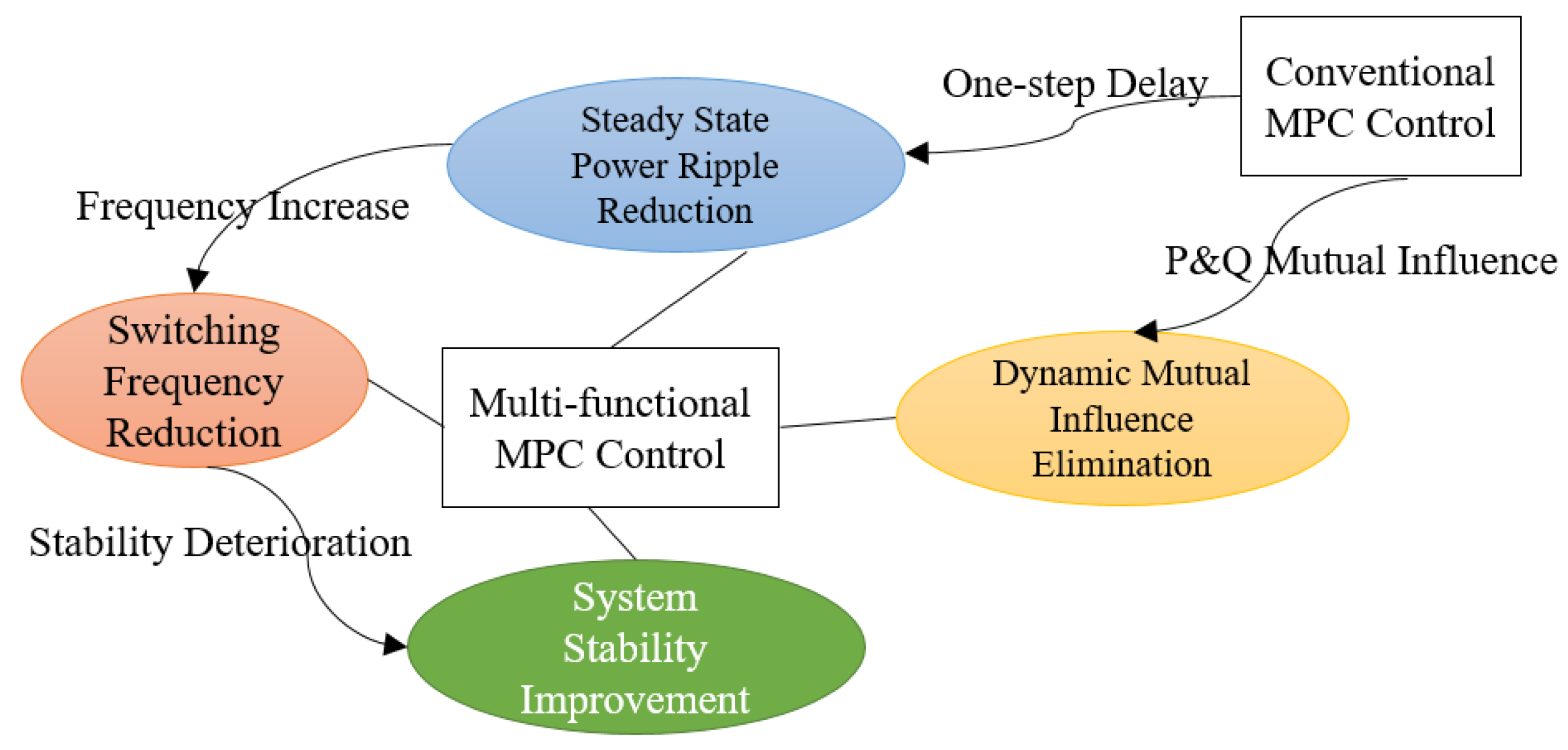
4. Proposed Multi-Functional MPC for Steady and Dynamic Performance Optimization

One of the main advantages of MPC is that any constraints or requirements for a prediction control can be included in the cost function to combine multiple constraints and nonlinearities together to improve the overall performance. The conventional MPC inherits two main issues which may influence the system performances. The first one is the influence on steady-state performance caused by one-step-delay in digital implementation, which results in large power ripples and higher current total harmonic distortion (THD) [34,35]. Though one-step-delay compensation can be added to solve this problem, the overall frequency increases obviously at the same time. Thus, we need to combine the switching frequency reduction constraint in the cost function with consideration of accompanying stability deterioration issue, thus the N step ahead prediction should be applied.

The second problem is the dynamic performance deterioration caused by the mutual influence between active and reactive powers due to the control coupling of two targets in the single cost function. The solution of dynamic performance issue is by adding the eliminating constraint, which will be introduced in the below section.

By overall consideration of steady-state and dynamic-state performance optimization, the proposed multi-functional MPC (MMPC) can improve both the steady-state and dynamic performance simultaneously in comparison with the conventional MPC control. The proposed MMPC constructs the redesigned cost function with additional objective terms in consideration of switching frequency reduction, one-step-delay compensation, and mutual influence elimination. The design loop of the proposed strategy is illustrated in Figure 3.

4.1. Steady-state Performance Improvement

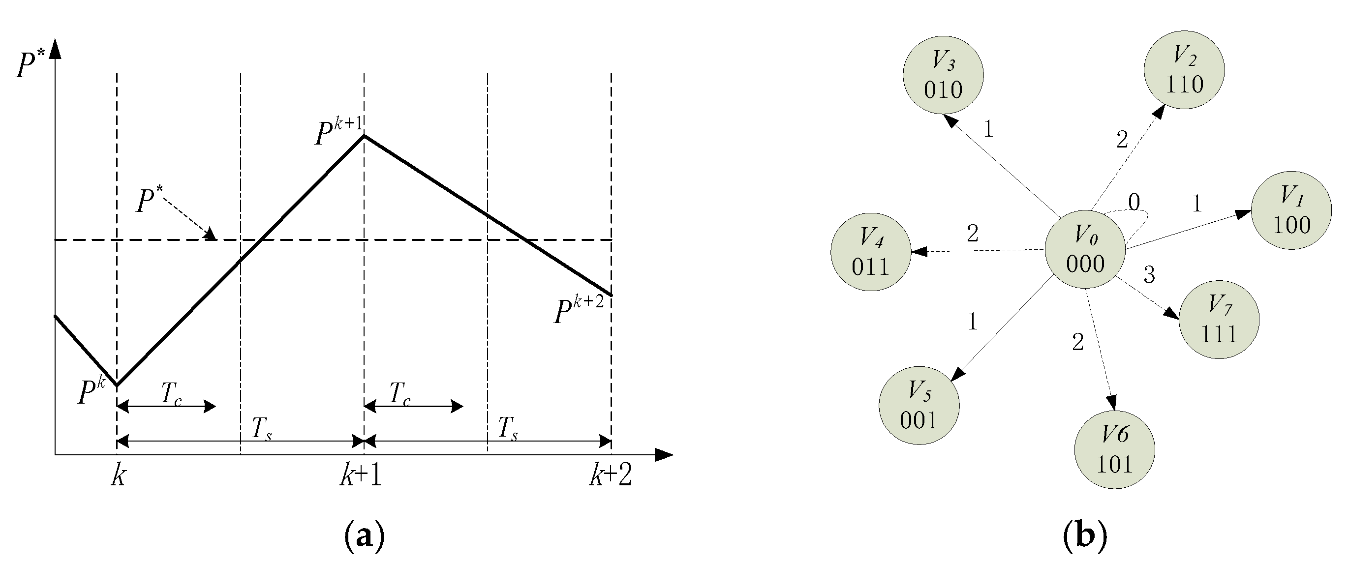
4.1.1. One-Step-Delay Compensation

For the steady-state performance, the most significant influence is caused by one-step-delay in discrete-time digital implementation. The one-step-delay issue exists when using (11) and (12) for real system control, which increases the power ripples in the steady-state, resulting in power prediction errors. Taking the active power as an example, as illustrated in Figure 4a, P^k is the sampled data at the k-th period, and T_c is the computing time of control strategy. After the best voltage vector $V_i^{k+1}$ is determined using P^k and P*, the best vector will be implemented at the (k+1)-th period while the active power variables at the (k+1)-th period are changed to P^k+1, which would be usually different from P^k because of the application of $V_i^k$. Therefore, the vector chosen at the (k+1)-th instant may no longer be the best one, and the one-step-ahead prediction value P^k+2 that is acquired through the converter model should be used in the cost function instead of P^k+1 to calculate the best vector for (k+1)-th instant. Likewise, the Q^k+2 acquired through the prediction model should be used in the cost function instead of Q^k+1 for the best vector selection.

With the one-step-delay compensation, the new cost function ${(J_0)}_i$ should be redefined as:

$${(J_0)}_i={(P^{*}-P_i{}^{k+2})}^2+{(Q^{*}-Q_i{}^{k+2})}^2$$

(13)

4.1.2. Frequency Reduction and Stability Improvement

While applying for the one-step-delay compensation, it is known that the switching frequency increases obviously [21]. The power losses of the converter increase with the increasing of switching frequency, especially in high power applications. The switching frequency can be reduced by seeking the minimum possible state changes of each switch [37]. Taking the switching state “000” as an example, Figure 4b shows the possible vector switching patterns. It can be seen there are four patterns based on the switch change’s number, i.e. the zero, one, two, and three state changes. To reduce the switch state change, the switching path which has the least leg switch changes is preferred.

According to the analyses above, the additional term ${(J_1)}_i$ can be further added:

$${(J_1)}_i={\lambda }_f\left({\displaystyle \sum _{i=a,b,c}\left|D_i^{k+1}-D_i^k\right|}\right)$$

(14)

where $D_i^k$ and $D_i^{k+1}$ mean the switching status of phase i (i=a, b, c) bridge leg in the k-th and (k+1)-th instants, respectively; $D_i^k$ = 0 or 1, where 1 means the higher switch is on and the lower switch is off, and 0 otherwise;${\lambda }_f$ is the weighting factor. Therefore, by redesigning the cost function as (14), the switching frequency reduction can be realized.

As indicated in Figure 3, the system control stability may deteriorate with the application of switching frequency reduction method, resulting in quite large power and current ripples [6]. A common solution is to predict the behavior of the variables with N steps ahead, by controlling the tracking error at the (k + N)-th (N >1) instant. The active and reactive powers at the (k + N)-th control period are derived linearly based on the value at the (k + 1)-th and (k + 2)-th control period. This could help reduce the system power ripples, especially when ${\lambda }_f$ is too large. Finally, for the steady-state performance improvement, the term (14) can be further revised to (15) as in [37]:

$$\{\begin{array}{l}{(J_1)}_i={\lambda }_f\left({\displaystyle \sum _{i=a,b,c}\left|D_i^{k+1}-D_i^k\right|}\right)+{\lambda }_s\left(\left|P^{*}-P_i{}^{k+N}\right|+\left|Q^{*}-Q_i{}^{k+N}\right|\right)\\ {(J_{0,1})}_i={(J_0)}_i+{(J_1)}_i\end{array}$$

(15)

where ${\lambda }_s$ is the weighting factor of stability, $P_i^{k+N}$ and $Q_i^{k+N}$ are the active and reactive powers at the (k + N)-th instant using the linear extrapolation for the prediction horizon. However, even at this stage with the revised cost function (15), only the steady-state performance is enhanced while the dynamic mutual influence has not been considered.

4.2. Dynamic Performance Improvement with Mutual Influence Elimination Constraint

In the above cost functions, the active and reactive power control are coupled in a single cost function and are controlled together to achieve the minimum cost function value. If one objective is significantly changed using MPC control with the aforementioned cost function, the control is targeted at the changing objective, while the other one is neglected. As a result, the transient performance would deteriorate obviously. The deterioration increases while the changing of the two control factors becomes larger, especially in the high power range. Due to such interference, the issue of dynamic performance deterioration should also be took into account.

To eliminate the mutual interference issue and enhance the dynamic performance of conventional MPC, a novel control constraint is proposed in this paper, which can be used as a general approach to eliminate the mutual influence in MPC by balancing the P and Q control. The eliminating constraint ${(J_2)}_i$ that resolves the mutual influence can be expressed as:

$${(J_2)}_i={\lambda }_m\left|(Q^{*}-Q_i{}^{k+2})(P^{*}-P_i{}^{k+2})\right|$$

(16)

The parameter ${\lambda }_m$ is the weighting factor of mutual influence elimination, it is chosen based on the system’s rated active and reactive powers. At the instant of a step change of $P^{*}$ or $Q^{*}$, the vector that may incur large mutual influence on the other control objective would be less considered. The constraint ${(J_2)}_i$ has almost no influence at steady-state.

Then the cost function (15) for improving steady-state performance could be further reorganized. Adding this term in the cost function to eliminate the mutual interference leads to the revised final cost function as:

$${(J_{0,1,2})}_i={(J_0)}_i+{(J_1)}_i+{(J_2)}_i$$

(17)

By selecting the voltage space vector which achieves the lowest cost function value of (17) after evaluation of all the voltage vectors, four separate optimization problems are solved comprehensively. In (17), each term has a corresponding weighting factor. In actual application, firstly, the selection of these weighting factors is through trial and error by simulation. Then, it could be implemented in the experiment and make adjustment accordingly. Finally, the selected weighting factors would be implemented in practical application. Each weighting factor value would have an influence on the weighting factor selection of the others, and the weighting factor values are in relation with system configurations, thus it is quite a complex task for the mathematical derivation and verification about the calculation of each weighting factor, which is out of scope of the main target of this paper, it will be researched in the future work. By selecting proper weighting factors, good dynamic and steady-state performance can be balanced in a systematic way. It is obvious that the additional terms would increase the computational burden compared with the conventional methods due to more complex cost function, especially in less capable hardware system. However, it could be solved by using general methods like machine code optimization once the control strategy has been programmed. In actual application with 20k sampling frequency, the increased computational burden does not affect the control implementation.

To the best knowledge of the authors, this is the first time in the literature where steady-state and dynamic performance improvements are implemented simultaneously. It should be noted that the proposed method for eliminating mutual influence could be used as a general solution to solve the mutual influence of two control objectives for various MPC-based control applications, such as electrical drive. In summary, the proposed multi-functional MPC method chooses the voltage vector according to the cost function which takes the dynamic and steady performance into account. The results of all the voltage vectors on power regulation will be compared so that the selected voltage vector will have the minimum cost function value to the system. The superior performance with the proposed method has been verified by simulation and experimental results.

5. Simulation Results

The abovementioned control strategies have been numerically simulated by MATLAB/Simulink tool. The main system parameters used in the simulation are listed in

Table 1. Electrical Parameter of Simulation.

Description	Name	Value
Resistance of reactor	R	510 mΩ
Inductance of reactor	L	4.2 mH
DC-bus capacitor	C	3500 μF
Load resistance	RL	50 Ω
Source voltage	e	110 V(peak)
Source voltage frequency	f	50 Hz
DC-bus voltage	Vdc	300 V
Weighting factor	λm	0.02
Weighting factor	λf	100
Weighting factor	λs	55

. The sampling frequency remains the same as 20 kHz. For simplicity, the conventional DPC method and conventional MPC-based DPC methods without one-step-delay compensation are denoted as “CDPC” and “CMPC-I”, which are used as a benchmark for comparison. The conventional MPC with only one-step-delay compensation and stability enhancement is denoted as “CMPC-II”, the conventional MPC with only proposed mutual influence elimination is denoted as “MMPC-I”, and the proposed multi-functional MPC with both steady-state and dynamic performance improvement as “MMPC-II”. For convenience, the power flow direction from the AC side to the DC load is supposed as positive.

To analyze both the steady and dynamic-state performances for each of the control strategies, the P*steps up from 0 kW to 4 kW at 0 s while the Q* remains at 0 kVar. After that, the active power decreases to −5 kW at 0.02 s, the reactive power boosts to 3 kVar at 0.04 s. At 0.06 s, the active power boosts from −5 kW to 7 kW, while the reactive power reduces to −4 kVar at 0.08 s. At 0.1 s, the active power decreases from 7 kW to 0 kW.

5.1. Steady-State Performance Comparison

To compare the steady-state performance, the AC side input current and reactive power in the simulation are presented from 0 s to 0.04 s to indicate the detailed power ripples. As we can see from Figure 5, both the active and reactive powers track their reference values with high accuracy. From Figure 5a, we can observe that the power ripple reduces and the line currents are more sinusoidal with CMPC-I method. By introducing the delay compensation, the performance is further improved with CMPC-II method.

While with MMPC-II control, the ripples of active and reactive powers in the steady-state are improved in comparison with CMPC-I and MMPC-I method, also it is almost the same as CMPC-II control, as shown in Figure 5c, which aligns well with theoretical analyses.

The switching frequency increases apparently with one-step-delay compensation, which correspondingly increases the switching costs. To compare the switching frequency reduction performance of each method, the switching frequency can be evaluated by measuring the state changes of one phase leg in fixed time and divided by 2. The comparison is conducted at 0.05 s as an example. The sample period of frequency calculation is every 0.01 s. It can be seen from

Table 2. Quantitative Comparison of Simulation Results.

Control	THD (%)	Prip (W)	Qrip (Var)	fsw (Hz)	Psht (W)	Qsht (Var)	Time (ms)
CDPC [8]	7.95↑	209.6↑	323.1↑	1472↓	600↓	580↓	3.6↑
CMPC-I [35]	5.92 *	143.2 *	244.3 *	1908 *	2020 *	1855 *	2.5 *
CMPC-II [35]	2.69↓	77.7↓	81.3↓	3201↑	1561↓	1812↓	2.7↑
MMPC-I	5.33→	152.3→	224.3→	1952→	541↓	185↓	3.3↑
MMPC-II	2.76↓	81.8↓	83.1↓	3291↑	310↓	170↓	3.2↑

↑: Increased; ↓: Decreased; →: Constant; *: Referenced.

the CMPC-I and MMPC-I control have lower switching frequency due to lack of one-step-delay compensation. With one-step-delay compensation and corresponding frequency reduction, the switching frequency of CMPC-II method is 3201. MMPC-II control also has a similar frequency in comparison with CMPC-II, which verifies that MMPC-II also has switching frequency reduction ability. The quantitative comparison of the steady-state performance such as current THD, average switching frequency, active and reactive power ripple at P = −5 kW, Q = 0 kVar are shown in Table 2. We can conclude that both the CMPC-II and MMPC-II strategies have the best steady-state performance with lower active and reactive power ripple as well as a more sinusoidal waveform.

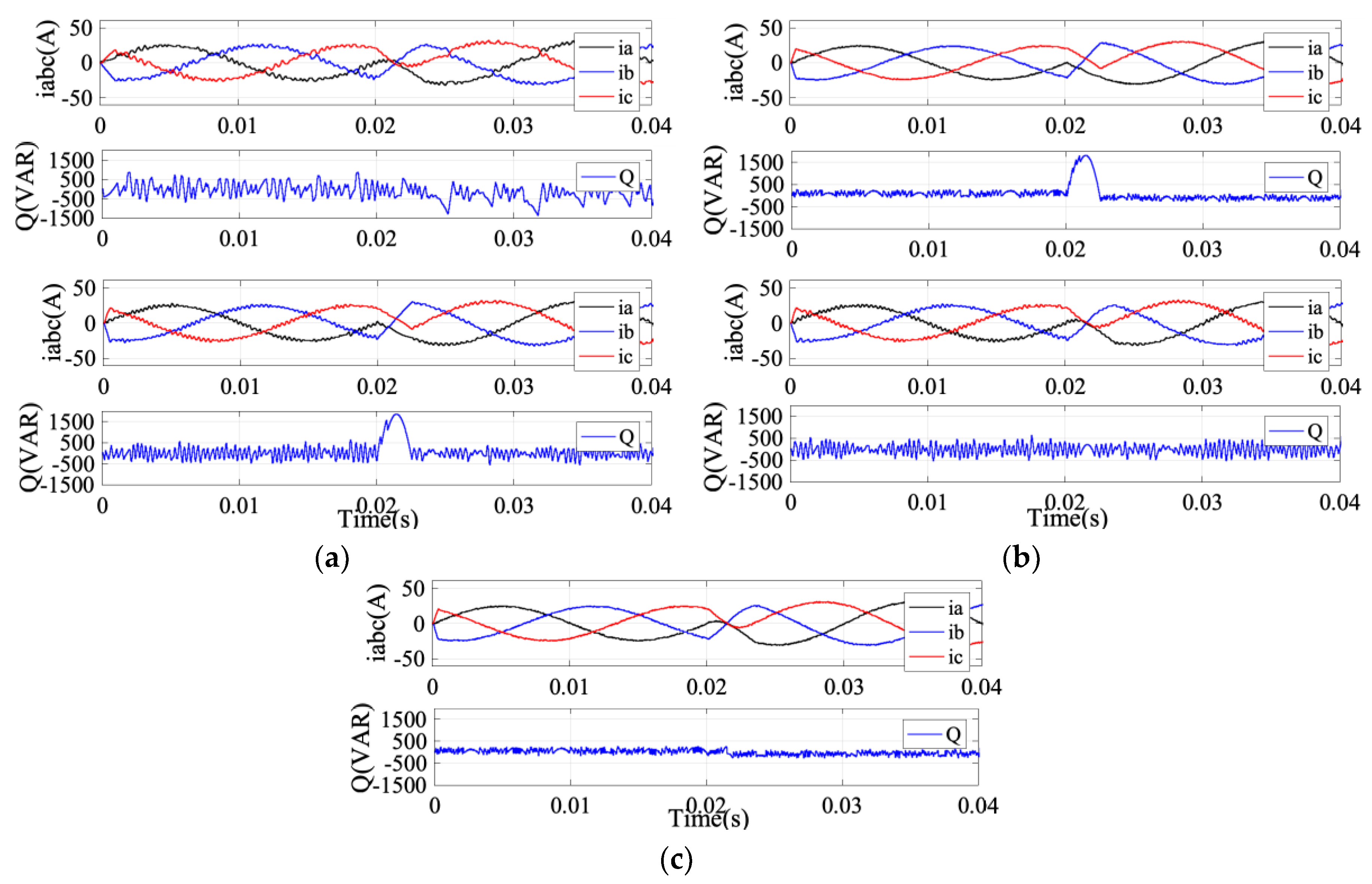
5.2. Dynamic Performance Comparison

To compare the transient performance, instantaneous responses of active and reactive power with each method are simulated, as in Figure 6. At transient instant, the sector where the mutual interference occurs is marked in dashed circle. The following comparisons of active power overshoot and reactive power overshoot take the instant of 0.06 s and 0.02 s as an example. As shown in Figure 6a, there is no obvious mutual influence between the active and reactive powers with CDPC control since the control of P and Q are decoupled; the active power overshoot is 580 W and reactive power overshoot is 600 Var. In comparison, the mutual influence of active and reactive power with the CMPC-I and CMPC-II is apparent at transient response of P and Q, as shown in solid circles in Figure 6b,c, the P and Q overshoot of CMPC-I are as high as 1855 W and 2020 Var, respectively.

With MMPC-I and MMPC-II, it achieves much better dynamic performance by eliminating mutual influence, as shown in Figure 6d,e. For instance, the active power overshoot is 310 W and reactive power overshoot is 170 Var with MMPC-II, which is significantly improved compared with CMPC-I and CMPC-II. Besides, MMPC-II has better dynamic performance in comparison with MMPC-I due to the improvement of steady-state performance simultaneously.

With the proposed MMPC-I and MMPC-II methods, the mutual influence between active and reactive powers is eliminated. There is almost no overshoot in both P and Q at step change conditions compared with CDPC and CMPC while keeping almost the same tracking quality. The quantitative comparison is presented in Table 2, the value of P overshoot is denoted as “Psht” and Q overshoot is denoted as “Qsht”, which takes the instances of 0.06 s and 0.02 as an example, respectively. In order to verify the desirable trends of these values according to the theoretical analyses, the CMPC-I method is selected as a reference and indicated by “*”, while the desirable trends of other methods compared with CMPC-I are indicated by the direction of arrows, as shown in Table 2. It can be concluded that the desirable trends of simulation results with each control method align well with the theoretical analyses, the switching frequency of MMPC-II increases obviously compared with conventional methods due to one-step-delay compensation, which means the switching loss would increase. In consideration of the overall control performance, the proposed MMPC-II is the best control strategy compared with others.

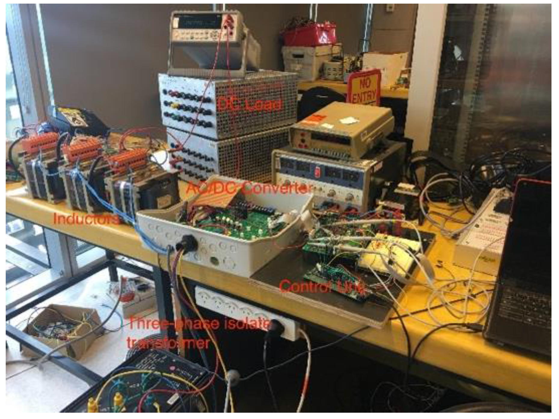
6. Experimental Results

To verify the performance of each strategy, a scaled-down prototype in the lab is constructed. The prototype is shown in Figure 7. A TMS320F28335 floating-point DSP manufactured by Texas Instrument from Dallas, Texas, USA is used for the control. The system parameter is presented in

Table 3. Electrical Parameter of Prototype.

Description	Name	Value
Resistance of reactor	R	500 mΩ
Inductance of reactor	L	22 mH
DC-bus capacitor	C	680 μF
Load resistance	RL	34 Ω
Source voltage	e	110 V(peak)
Sampling Period	Ts	50 μs
Source voltage frequency	f	50 Hz

. To compare the steady and dynamic performance of existing methods and the proposed method, a series of experiments have been done. The sampling frequency for each control method keeps the same as 20 kHz.

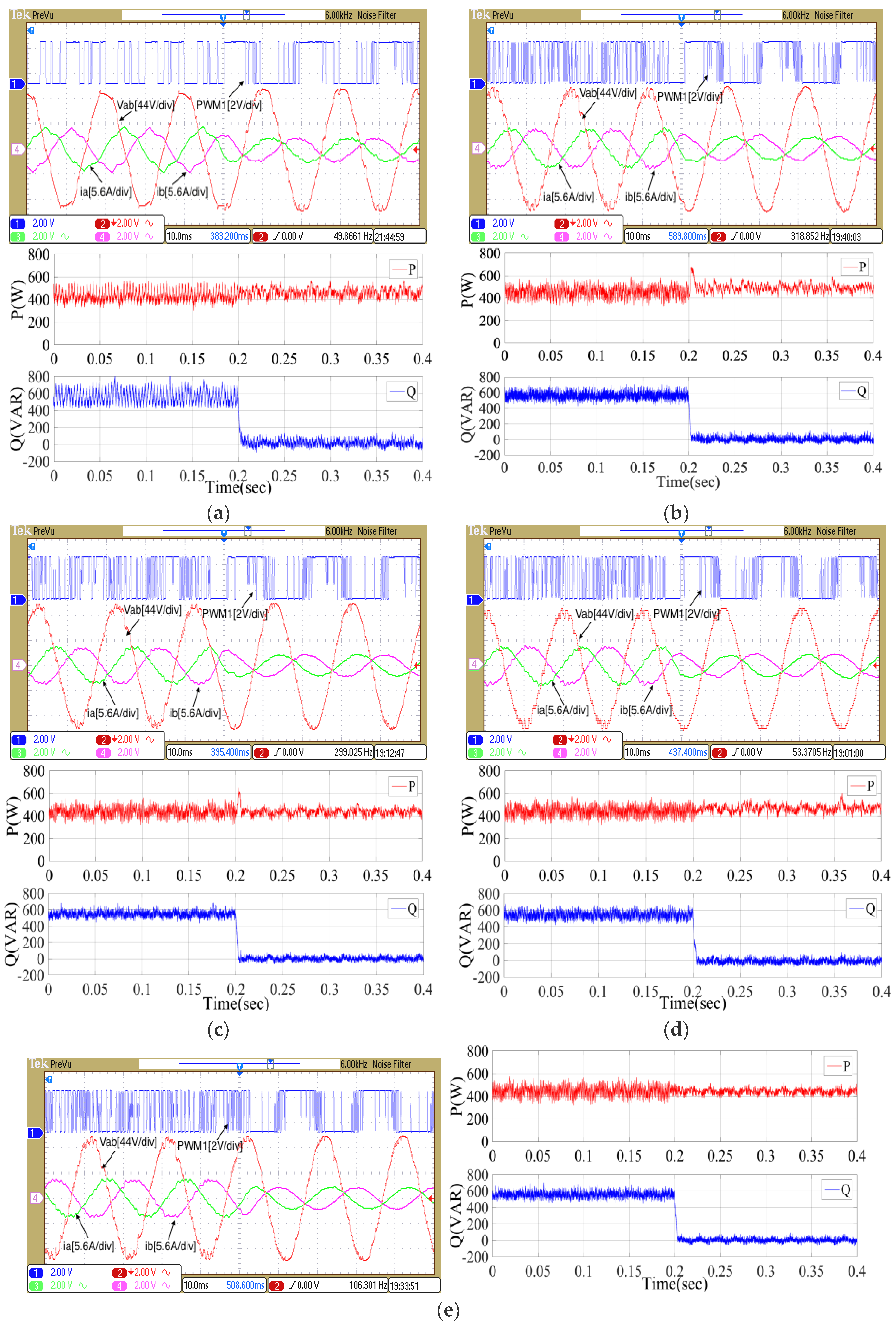
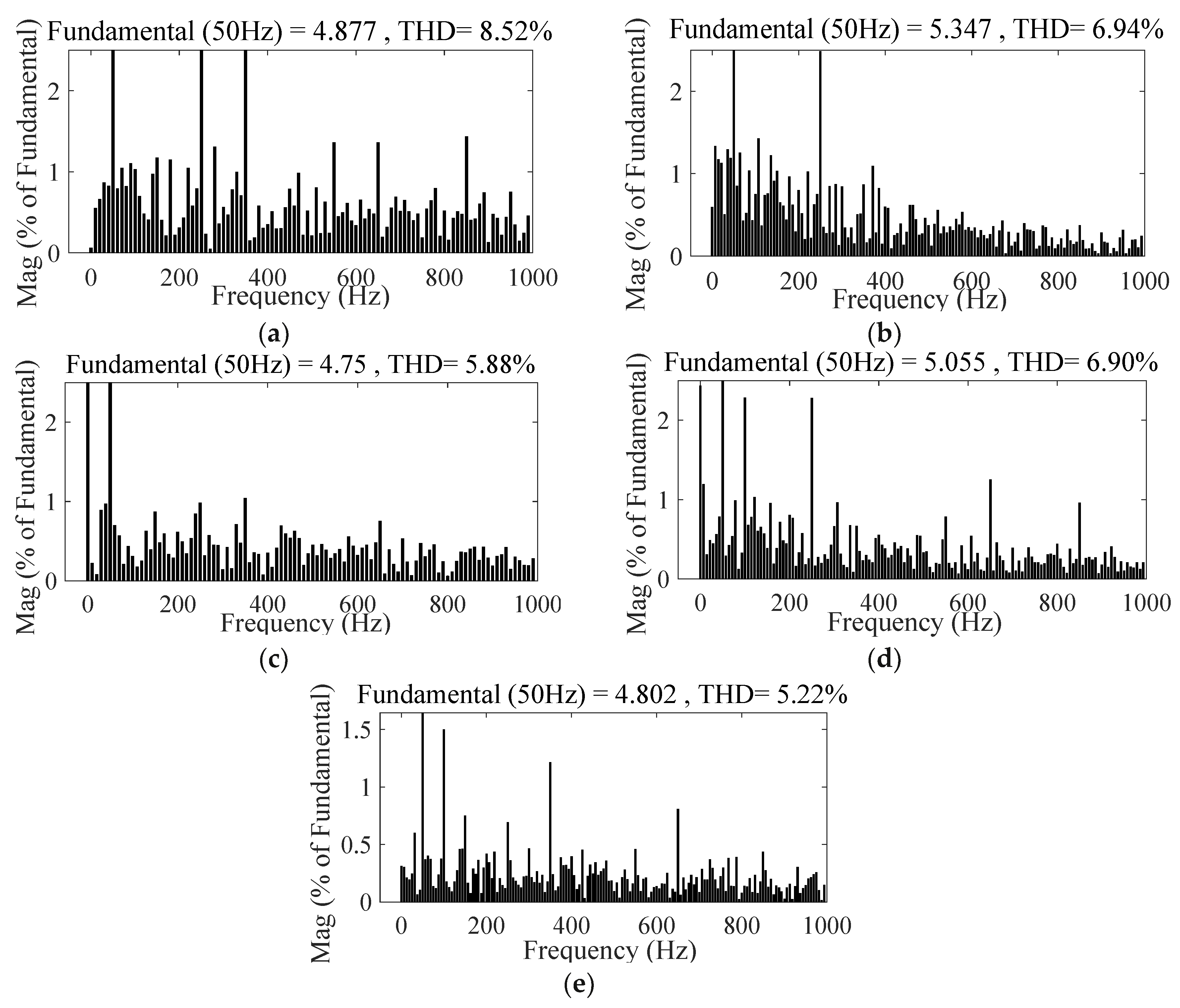
6.1. Comparison of Steady and Dynamic Performance under the Step Change of Reactive Power

For the steady-state performance, the current THD, power ripple of reactive power and active power and switching frequency comparison at steady-state of P = 450 W and Q = 0 Var have been conducted with each strategy. To compare the dynamic-state performance of each control method with Q step change, keep P* steady at 450 W and change the Q* from 550 Var to 0 Var at 0.2 s.

Figure 8a presents the upper switch driving signal of one leg, input line voltage V_ab, and input current i_a and i_b with CDPC method. It can be seen that both P and Q track their references successfully during the whole period. The current THD is 8.52% as shown in Figure 9a. The P and Q ripple is 38.56 W and 38.7 Var, respectively. The average switching frequency f_sw is 1720 Hz. For the dynamic performance, as shown in Figure 8a, CDPC method tracks the reference successfully within 0.0041s, there is no obvious mutual influence between P and Q control. The P overshoot when Q changes from 550 Var to 0 Var at 0.2 s is 68 W.

In comparison, the experimental result with CMPC-I method is shown in Figure 8b. It can be seen the steady-state performance is slightly improved in comparison with CDPC. The current THD is decreased to 6.94% as shown in Figure 9b, and the P ripple is decreased obviously to 30.59 W while the Q ripple is reduced to 31.57 Var. The average switching frequency f_sw is 2520 Hz. The dynamic performance of CMPC-I shows that the response time is 0.0027 s, the influence on P control is obvious while Q changes from 550 Var to 0 Var. The P overshoot is dramatically increased to 231 W at 0.2 s.

Similarly, the experimental result with CMPC-II method is shown in Figure 8c. It can be seen the steady-state performance is further improved in comparison with CMPC-I. The THD is 5.88% as shown in Figure 9c. The P ripple is 28.67 W, and the Q ripple is decreased to 22.87 Var. The average switching frequency f_sw is 3410 Hz. For the dynamic performance of CMPC-II method, the result indicates that the response time is 0.0032s, and the P overshoot is also as high as 201 W while Q has the step change at 0.2 s.

The experimental result with the proposed MMPC-I is shown in Figure 8d. The THD is 6.9% as shown in Figure 9d. The P and Q ripple is 32.82 W and 27.43 Var, respectively. The average switching frequency f_sw is 2650 Hz. It can be concluded that the steady-state performance is similar to that of CMPC-I method, which is deteriorated compared with CMPC-II control. While for the dynamic performance, the influence on the active power overshoot is significantly decreased to 71 W at the instance of Q step change in comparison with CMPC-I and CMPC-II method.

The experimental result with the proposed MMPC-II method is shown in Figure 8e, the THD is 5.22% as shown in Figure 9e. The P and Q ripple is 22.12 W and 22.49 Var, respectively, the average switching frequency is 3760 Hz. It is shown that the steady-state performance is improved obviously compared with CMPC-I, which is similar to CMPC-II. For the dynamic performance of MMPC-II, the P overshoot is significantly decreased to the lowest value of 49 W due to both the mutual influence elimination and steady-state performance improvement.

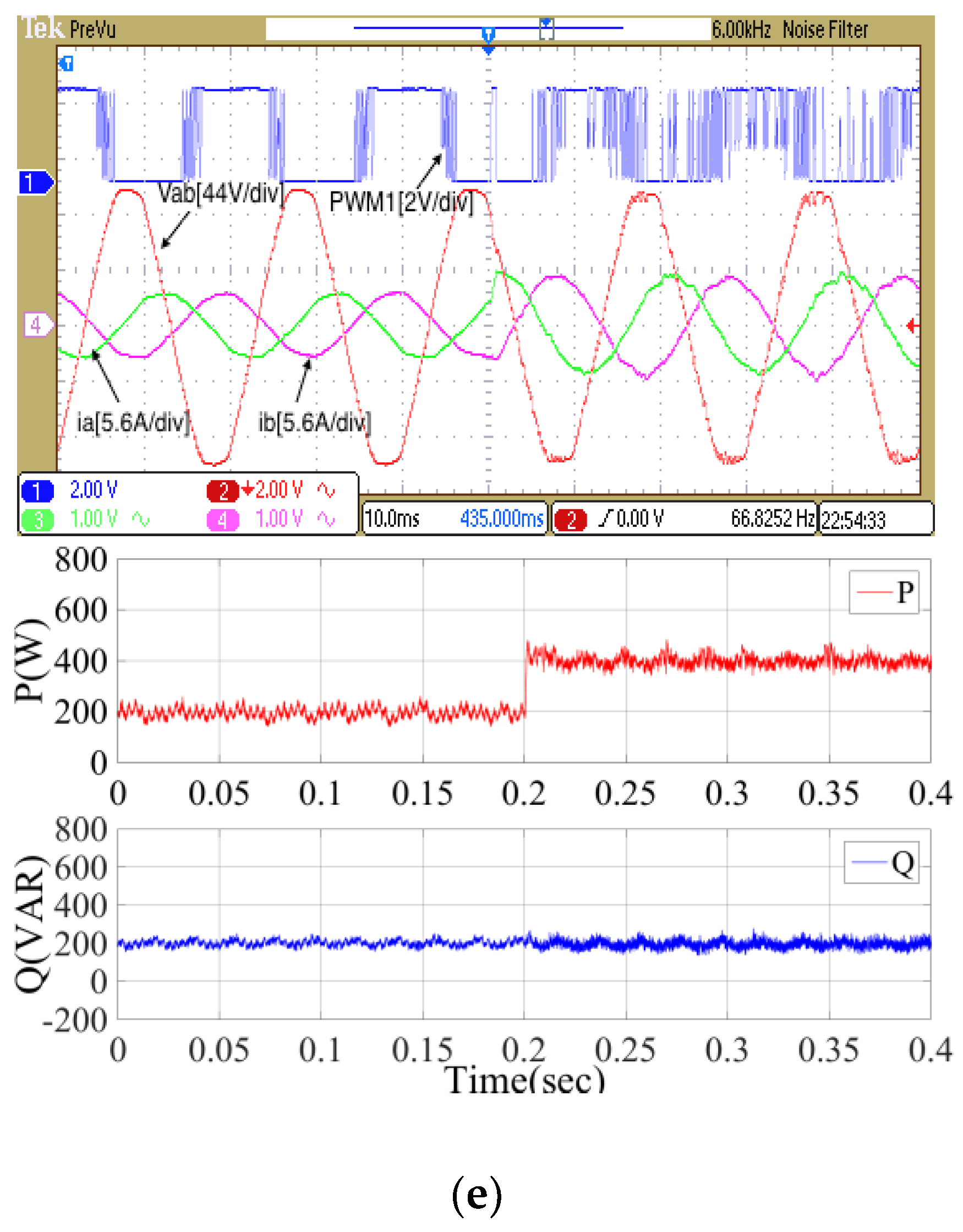
6.2. Dynamic-State Performance with P Step Change

To compare the influence on Q control when P has a step change. The experimental results with each control method have also been presented when Q reference keeps at 200 Var, and P reference steps up from 200 W to 400 W, as shown in Figure 10. With CDPC, the Q overshoot is 133 Var during the active power step change, as shown in Figure 10a. It is increased to 163 Var and 141 Var with CMPC-I and CMPC-II method, respectively, as shown in Figure 10b,c, while with the proposed MMPC-I and MMPC-II control strategies, the Q overshoot is significantly decreased to 45 Var and 49 Var, respectively, as shown in Figure 10d and Figure 10e, which verifies the simulation results well and validates the effectiveness of the proposed MMPC strategy.

The quantitative comparisons of steady and dynamic performance are presented in

Table 4. Quantitative Comparison of Steady-State and Dynamic-State Performance in Experiment.

Control	THD (%)	Prip (W)	Qrip (Var)	fsw (Hz)	Psht (W)	Qsht (Var)	Time (ms)
CDPC [8]	8.52↑	38.56↑	38.7↑	1720↓	68↓	133↓	4.1↑
CMPC-I [35]	6.94 *	30.59 *	31.57 *	2520 *	231 *	163 *	2.7*
CMPC-II [35]	5.88↓	28.67↓	22.87↓	3410↑	201↓	141↓	3.2↑
MMPC-I	6.90→	32.82→	27.43→	2650→	71↓	45↓	3.9↑
MMPC-II	5.22↓	22.12↓	22.49↓	3760↑	49↓	49↓	3.8↑

↑: Increased; ↓: Decreased; →: Constant; *: Referenced.

, which aligns well with the theoretical analyses and simulation results and well verified the proposed method with multi-functions.

7. Conclusions

In this paper, a multi-functional MPC strategy for three-phase AC/DC converters to improve the steady and dynamic performances simultaneously has been proposed. The steady and dynamic-state performances of CDPC, CMPC-I, CMPC-II, MMPC-I, and MMPC-II for different power levels are compared in both simulation and experiments. The proposed MMPC-I and MMPC-II methods have been verified to be able to eliminate the mutual influence of active and reactive power control. The proposed mutual influence elimination constraint is promising to be generally applied in MPC-based control for various control areas to eliminate mutual influence between different control objectives. Besides, the simulation and experimental results verify the proposed MMPC-II method has superior steady and dynamic performances compared with other methods by simultaneously reducing power variations and eliminating the mutual influence of active and reactive power at the dynamic-states.

References

1. Carrasco, J.M.; Franquelo, L.G.; Bialasiewicz, J.T.; Galvan, E.; Guisado, R.C.P.; Prats, A.M.; Leon, J.I.; Moreno-Alfonso, N. Power-electronic systems for the grid integration of renewable energy sources: A survey. IEEE Trans. Ind. Electron. 2006, 53, 1002–1016. [Google Scholar] [CrossRef]
2. Blaabjerg, F.; Liserre, M.; Ma, K. Power electronics converters for wind turbine systems. IEEE Trans. Ind. Appl. 2012, 48, 708–719. [Google Scholar] [CrossRef]
3. Rodriguez, J.R.; Dixon, J.W.; Espinoza, J.R.; Pontt, J.; Lezana, P. PWM regenerative rectifiers: State of the art. IEEE Trans. Ind. Electron. 2005, 52, 5–22. [Google Scholar] [CrossRef]
4. Blaabjerg, F.; Teodorescu, R.; Liserre, M.; Timbus, A.V. Overview of control and grid synchronization for distributed power generation systems. IEEE Trans. Ind. Electron. 2006, 53, 1398–1409. [Google Scholar] [CrossRef]
5. Chakraborty, S.; Kramer, B.; Kroposki, B. A review of power electronics interfaces for distributed energy systems toward achieving low-cost modular design. Renew. Sustain. Energy Rev. 2009, 13, 2323–2335. [Google Scholar] [CrossRef]
6. Strasser, T.; Andrén, F.; Kathan, J.; Cecati, C.; Buccella, C.; Siano, P.; Leitão, P.; Zhabelova, G.; Vyatkin, V.; Vrba, P.; et al. A Review of Architectures and Concepts for Intelligence in Future Electric Energy Systems. IEEE Trans. Ind. Electr. 2015, 62, 2424–2438. [Google Scholar] [CrossRef] [Green Version]
7. Alonso-Martinez, J.; Carrasco, J.E.; Arnaltes, S. Table-based direct power control: A critical review for microgrid applications. IEEE Trans. Power Electron. 2010, 25, 2949–2961. [Google Scholar] [CrossRef]
8. Zhang, Y.; Li, Z.; Zhang, Y.; Xie, W.; Piao, Z.; Hu, C. Performance improvement of direct power control of PWM rectifier with simple calculation. IEEE Trans. Power Electron. 2013, 28, 3428–3437. [Google Scholar] [CrossRef]
9. Hu, J.; Zhu, J.; Dorrell, D.G. A Comparative Study of Direct Power Control of AC/DC Converters for Renewable Energy Generation. Proc. IEEE IECON Conf. 2011, 3453–3458. [Google Scholar] [CrossRef]
10. Noguchi, T.; Tomiki, T.; Kondo, S.; Takahashi, I. Direct power control of PWM converter without power-source voltage sensors. IEEE Trans. Ind. Appl. 1998, 34, 473–479. [Google Scholar] [CrossRef]
11. Xu, L.; Zhi, D.; Yao, L. Direct power control of grid connected voltage source converters. Proc. IEEE Power Eng. Soc. Gen. Meet. 2007, 1–6. [Google Scholar] [CrossRef]
12. Malinowski, M.; Kazmierkowski, M.P.; Trzynadlowski, A.M. A comparative study of control techniques for PWM rectifiers in AC adjustable speed drives. IEEE Trans. Power Electron. 2003, 18, 1390–1396. [Google Scholar] [CrossRef]
13. Antoniewicz, P.; Kazmierkowski, M. Virtual-flux-based predictive direct power control of ac/dc converters with online inductance estimation. IEEE Trans. Ind. Electron. 2008, 55, 4381–4390. [Google Scholar] [CrossRef]
14. Hu, J.; Zhu, J.; Dorrell, D.G. In-depth study of direct power control strategies for power converters. IET Power Electronics. 2014, 7, 1810–1820. [Google Scholar] [CrossRef]
15. Vazquez, S.; Rodriguez, J.; Rivera, M.; Franquelo, L.G.; Norambuena, M. Model predictive control for power converters and drives: Advances and trends. IEEE Trans. Ind. Electron. 2017, 64, 935–947. [Google Scholar] [CrossRef]
16. Kouro, S.; Cores, P.; Vargas, R.; Ammann, U.; Rodrıguez, J. Model predictive control—A simple and powerful method to control power converters. IEEE Trans. Ind. Electron. 2009, 56, 1826–1838. [Google Scholar] [CrossRef]
17. Zhang, Y.; Xie, W.; Li, Z.; Zhang, Y. Model predictive direct power control of a PWM rectifier with duty cycle optimization. IEEE Trans. Power Electron. 2013, 28, 5343–5351. [Google Scholar] [CrossRef]
18. Zhang, Y.; Xie, W. Low complexity model predictive control—Single vector based approach. IEEE Trans. Power Electron. 2014, 29, 5532–5541. [Google Scholar] [CrossRef]
19. Song, Z.; Xia, C.; Liu, T. Predictive current control of three-phase grid- connected converters with constant switching frequency for wind energy systems. IEEE Trans. Ind. Electron. 2013, 60, 2451–2464. [Google Scholar] [CrossRef]
20. Aguilera, R.P.; Lezana, P.; Quevedo, D.E. Finite-control-set model predictive control with improved steady-state performance. IEEE Trans. Ind. Electron. 2013, 9, 658–667. [Google Scholar] [CrossRef]
21. Preindl, M.; Schaltz, E.; Thøgersen, P. Switching frequency reduction using model predictive direct current control for high-power voltage source inverters. IEEE Trans. Ind. Electron. 2011, 58, 2826–2835. [Google Scholar] [CrossRef]
22. Cortes, P.; Ortiz, G.; Yuz, J.; Rodriguez, J.; Vazquez, S.; Franquelo, L.G. Model predictive control of an inverter with output LC filter for UPS applications. IEEE Trans. Ind. Electron. 2009, 56, 1875–1883. [Google Scholar] [CrossRef]
23. Vazquez, S.; Montero, C.; Bordons, C.; Franquelo, L.G. Model predictive control of a VSI with long prediction horizon. Proc. IEEE Int. Symp. Ind. Electron. 2011, 1805–1810. [Google Scholar] [CrossRef]
24. Hu, J.; Zhu, Z. Improved voltage-vector sequences on dead-beat predictive direct power control of reversible three-phase grid-connected voltage-sourced converters. IEEE Trans. Power Electron. 2013, 28, 254–267. [Google Scholar] [CrossRef]
25. Song, Z.; Chen, W.; Xia, C. Predictive direct power control for three-phase grid-connected converters without sector information and voltage vector selection. IEEE Trans. Power Electron. 2014, 29, 5518–5531. [Google Scholar] [CrossRef]
26. Ramirez, R.O.; Espinoza, J.R.; Villarroel, F.; Maurelia, E.; Reyes, M.E. A novel hybrid finite control set model predictive control scheme with reduced switching. IEEE Trans. Ind. Electron. 2014, 61, 5912–5920. [Google Scholar] [CrossRef]
27. Rodriguez, J.; Kazmierkowski, M.P.; Espinoza, J.R.; Zanchetta, P.; Abu-Rub, H.; Young, H.A.; Rojas, C.A. State of the art of finite control set model predictive control in power electronics. IEEE Trans. Ind. Informat. 2013, 9, 1003–1016. [Google Scholar] [CrossRef]
28. Maedera, U.; Borrelli, F.; Morari, M. Linear offset-free model predictive control. Automatica 2009, 45, 2214–2222. [Google Scholar] [CrossRef]
29. Larrinaga, S.A.; Rodriguez, M.A.; Oyarbide, E.; Apraiz, J.R.T. Predictive control strategy for DC/AC converters based on direct power control. IEEE Trans. Ind. Electron. 2007, 54, 1261–1271. [Google Scholar] [CrossRef]
30. Cortes, P.; Kazmierkowski, M.; Kennel, R.; Quevedo, D.; Rodriguez, J. Predictive control in power electronics and drives. IEEE Trans. Ind. Electron. 2008, 55, 4312–4324. [Google Scholar] [CrossRef]
31. Kwak, S.; Park, J.-C. Switching strategy based on model predictive control of VSI to obtain high efficiency and balanced loss distribution. IEEE Trans. Power Electron. 2014, 29, 4551–4567. [Google Scholar] [CrossRef]
32. Vazquez, S. Model predictive control: A review of its applications in power electronics. IEEE Ind. Electron. Mag. 2014, 8, 16–31. [Google Scholar] [CrossRef]
33. Vazquez, S.; Sanchez, J.A.; Carrasco, J.M.; Leon, J.I.; Galvan, E. A model-based direct power control for three-phase power converters. IEEE Trans. Ind. Electron. 2008, 55, 1647–1657. [Google Scholar] [CrossRef]
34. Abu-Rub, H.; Guzinski, J.; Krzeminski, Z.; Toliyat, H.A. Predictive current control of voltage source inverters. IEEE Trans. Ind. Electron. 2004, 51, 585–593. [Google Scholar] [CrossRef]
35. Hu, J.; Zhu, J.; Platt, G.; Dorrell, D.G. Multi-objective model-predictive control for high power converters. IEEE Trans. Energy Convers. 2013, 28, 652–663. [Google Scholar] [CrossRef]
36. Quevedo, D.E.; Aguilera, R.P.; Perez, M.A.; Cortes, P.; Lizana, R. Model predictive control of an AFE rectifier with dynamic references. IEEE Trans. Power Electron. 2012, 27, 3128–3136. [Google Scholar] [CrossRef]
37. Cortes, P.; Rodriguez, J.; Antoniewicz, P.; Kazmierkowski, M. Direct power control of an AFE using predictive control. IEEE Trans. Power Electron. 2008, 23, 2516–2523. [Google Scholar] [CrossRef]
38. Choi, D.; Lee, K. Dynamic performance improvement of AC/DC converter using model predictive direct power control with finite control set. IEEE Trans. Ind. Electron. 2015, 62, 757–767. [Google Scholar] [CrossRef]
Figure 1. (a) AC/DC three-phase converter topology. (b) Voltage space vectors.
Energies 12 01616 g001
Figure 2. Block diagram of MPC-based power regulation.
Energies 12 01616 g002
Figure 3. MMPC control design in comparison with CMPC.
Energies 12 01616 g003
Figure 4. (a). Data processing in digital implementation. (b). switching paths.
Energies 12 01616 g004
Figure 5. From top to bottom. (a) CDPC three-phase currents, CDPC reactive powers, CMPC-I three-phase currents, CMPC-I reactive powers; (b) CMPC-II three-phase currents, CMPC-II reactive powers, MMPC-I three-phase currents, MMPC-I reactive powers; (c) MMPC-II three-phase currents, MMPC-II reactive powers.
Energies 12 01616 g005
Figure 6. Dynamic performance. From top to bottom, AC voltage, three-phase currents, active power, and reactive power. (a) CDPC. (b) CMPC-I. (c) CMPC-II. (d) MMPC-I. (e) MMPC-II.
Energies 12 01616 g006
Figure 7. Laboratory experimental prototype.
Energies 12 01616 g007
Figure 8. Experimental results when P = 450 W, Q changes from 550 Var to 0 Var. Top: PWM signal, V a b , i a and i b . Bottom: active and reactive power. (a) CDPC. (b) CMPC-I. (c) CMPC-II (d) MMPC-I. (e) MMPC-II.
Energies 12 01616 g008
Figure 9. Harmonic spectra of AC current when P = 450 W, Q = 0 Var. (a) CDPC. (b) CMPC-I. (c) CMPC-II (d) MMPC-I (e) MMPC-II.
Energies 12 01616 g009
Figure 10. Experimental results when Q = 200 Var, P changes from 200 W to 400 W. Top: PWM signal, V a b , i a and i b . Bottom: active and reactive power. (a) CDPC. (b) CMPC-I. (c) CMPC-II. (d) MMPC-I. (e) MMPC-II.
Energies 12 01616 g010aEnergies 12 01616 g010b