Abstract
The purpose of this paper is to remove the exponentially decaying DC offset in fault current waveforms using a deep neural network (DNN), even under harmonics and noise distortion. The DNN is implemented using the TensorFlow library based on Python. Autoencoders are utilized to determine the number of neurons in each hidden layer. Then, the number of hidden layers is experimentally decided by comparing the performance of DNNs with different numbers of hidden layers. Once the optimal DNN size has been determined, intensive training is performed using both the supervised and unsupervised training methodologies. Through various case studies, it was verified that the DNN is immune to harmonics, noise distortion, and variation of the time constant of the DC offset. In addition, it was found that the DNN can be applied to power systems with different voltage levels.
1. Introduction
While the consumption of electrical energy is increasing day by day, other factors such as power quality and reliability also need to be improved. Protective devices have been improved dramatically as time has passed by to protect power systems and to provide continuous power supply to users. However, variation of current magnitude, known as DC offset, sometimes confuses the operation of protective devices, which leads to miss-operation or unnecessary power outage due to the inaccuracy of current phasor estimation, which is the fundamental for operating modern protective devices. In order to get better accuracy estimation, this paper proposes a method for constructing, training, and testing a deep neural network (DNN) for removing the exponentially decaying DC offset in the current waveform when a power system fault occurs.
Background
In recent decades, various algorithms and methods have been proposed to deal with the DC offset problem [1,2,3,4,5,6,7,8,9,10,11,12,13,14,15,16,17]. An approach to remove the DC offset from fault current waveforms is to modify their discrete Fourier transform (DFT) in the phasor domain [2,3,4,5,6,7,8,9,10,11]. Most phasor-domain algorithms remove DC offset by analyzing the relationship between the real and imaginary parts of the phasor. By taking advantages of the superior performance of the DFT, phasor-domain algorithms can effectively eliminate DC offset and provide smooth transient response. These algorithms are also robust against noise, but the disadvantage is that the phasor estimation needs more than one cycle.
Another approach is to remove the DC offset directly in the time domain [12,13,14,15,16,17]. Most time-domain algorithms significantly remove the DC offset faster than phasor-domain algorithms. Phasor estimation can also be achieved in the time domain, either simultaneously with or directly after removing the DC offset [12,13,14]. These methods provide a fast response, but are prone to errors when the fault current waveform contains high-frequency components. To overcome this drawback, some algorithms remove the DC offset in the time domain, then apply the DFT for phasor estimation [15,16,17]. Similar to phasor-domain algorithms, these new algorithms effectively eliminate DC offset. However, the time delay imposed by performing the DC offset removal and DFT leads to taking more than one cycle to estimate the phasor.
In order to eliminate the time delay while removing the DC offset in the time domain, the DNN method has been proposed in this paper. The DNN output is the signal of current waveform after removing the DC offset without any time delay. The non-DC offset output is then applied as an input for DFT-based phasor estimation algorithm. In addition to the nonlinearity of the DC offset, the phasor estimation accuracy is usually affected by random noise, which is frequently caused by the analog to digital conversion (ADC) process [18]. As DNN is one of the most effective solutions for nonlinear applications [19,20,21,22,23], it will be chosen to deal with the nonlinearity of DC offset. In this study, in order to improve the training speed through parallel computation [24], a CPU NVIDIA GTX 1060 graphics processing unit has been used for training the DNN.
The details of proposed method, experiment procedures, and results will be discussed in the following sections. Section 2 will explain the preparation of the training data, while the structure and DNN training will be demonstrated in Section 3. The results and conclusion are provided in Section 4 and Section 5, respectively.
2. Data Acquisition
There are four stages of training data preparation: data generation, moving window formation, normalization, and random shuffling. As the training datasets have a considerable influence on the performance of DNN, there should be a sufficient amount of data of the required quality, such that the training process can find a good local optimum that satisfies every training dataset given to the DNN. In this study, the theoretical equations for each component (DC offset, harmonics, and noise) were modeled using Python code and training data were acquired directly through iterative simulations.
2.1. Data Generation
We modeled a simple single-phase RL circuit (60 Hz) to simulate power system faults with DC offset, harmonics, and noise based on theoretical equations. It was designed to manually determine the time constant, fault inception angle, number of harmonics, and amount of noise. The modeling result is then compared with that of PSCAD/EMTDC simulation. The results show that the modeling single-phase RL (60 Hz) is adequate to apply for simulation based on the theorical condition.
2.1.1. Exponentially Decaying DC Offset
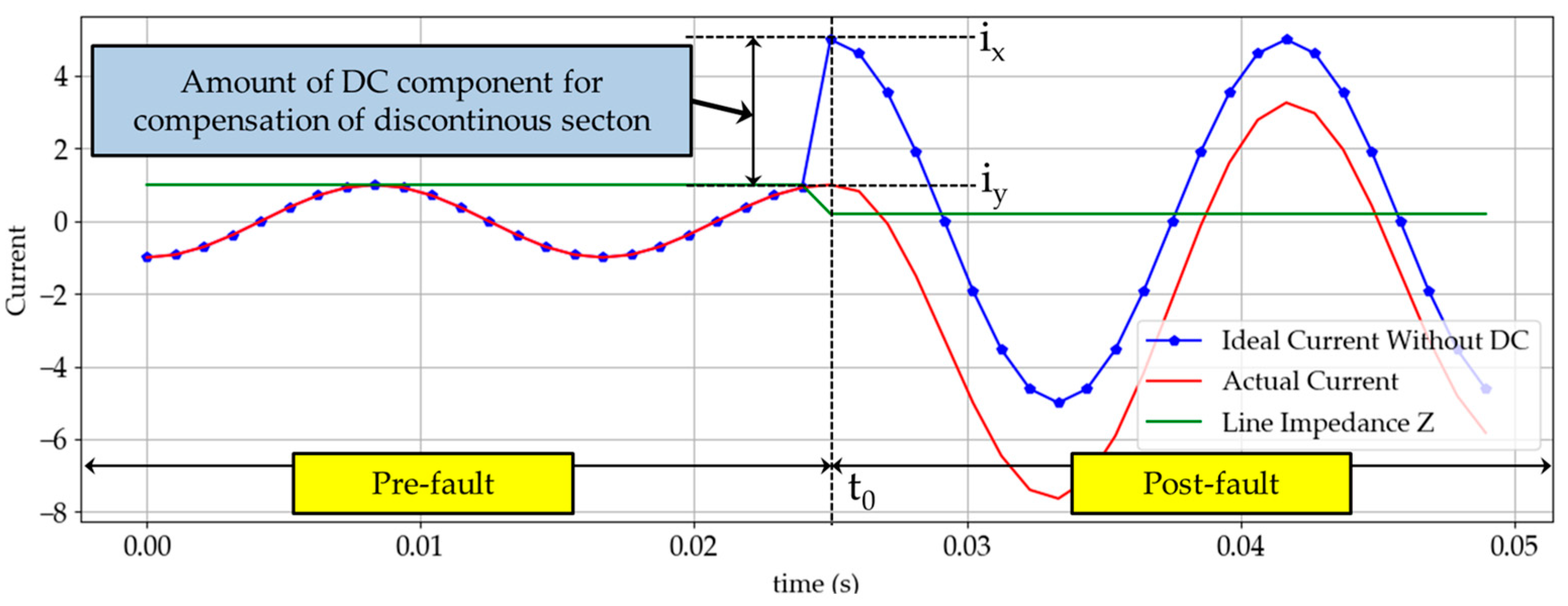
It is well known that DC offset occurs in current waveform during faults in a power system. The fault current with DC offset after fault inception time t0 is given in (1), and its illustration is shown in Figure 1 and Figure 2.
where is the angle of the RL circuit, which is near to 90°; and is the inception angle.
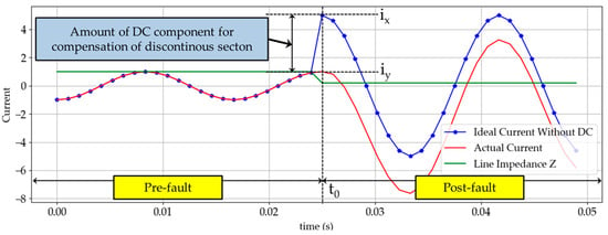
Figure 1.
Current increasing during fault occurs at t0 (fault inception angle 0°).

Figure 2.
Exponentially decaying DC offset at different fault inception angles: (a) fault inception angle of 180°; (b) fault inception angle of 90°.
A sudden increase in current causes a discontinuous section in the waveform. However, according to Faraday’s Law of Induction, the current flowing in the line cannot change instantaneously in the presence of line inductance. This is the main cause of the DC offset, and the initial value of the DC offset depends on the fault inception angle, while its decay rate depends on the time constant of the power system. Particularly, Figure 2b demonstrates fault current when the inception angle is 90° and its waveform is similar to fault current waveform without DC offset. Assuming that there is no current just before the fault inception time , the DC offset given in (1) is almost zero because is near to zero.
2.1.2. Harmonics
Harmonics are defined in the works of [25] as sinusoidal components of a periodic wave or quantity having a frequency that is an integral multiple of the fundamental frequency, and can be expressed as follows:
where n is the harmonic order and An is its amplitude. The second, third, fourth and fifth harmonic components were considered in this paper to maintain an acceptable training speed.
2.1.3. Additive Noise
There are many types of noise interference; however, the typical noise type in power system measurements is quantization noise [26] in AD conversion. As noise components have no specified frequency, it was approximated as additive Gaussian white noise (AGWN) and the amount of noise was adjusted by setting the signal-to-noise ratio (SNR), which can be expressed as follows:
The noise component will disrupt the normal operation of digital filtering algorithms, as discussed in earlier sections.
2.1.4. Simulation
On the basis of the theories discussed above, we modeled a simple RL circuit in Python code using NumPy for the simulation of current waveforms. Then, we iterated over the parameters shown in Table 1 to obtain a range of situations that can occur in a power system. As shown in Table 1, the total number of performing simulations is 6480. For simple rehearsal training, the parameters are selected less strictly to maintain an acceptable training speed.

Table 1.
Parameters for generating the training datasets. SNR—signal-to-noise ratio.
The validation datasets were generated using the same methodology as the training datasets; however, the validation datasets do not include any of the training datasets. Their generation was conducted by iterating over the parameters given in Table 2.

Table 2.
Parameters for generating the validation datasets.
2.2. Pre-Processing
Pre-processing includes moving window formation, normalization, and random shuffling. This process was carried out to generate training data in a form suitable for implementing a DNN. In this paper, the DNN was planned to reconstruct an output of one cycle corresponding to the fundamental current waveform when the DNN received one cycle of the current waveform including DC offset, harmonics, and noise. As 64 samples/cycle was decided as the sampling rate, the size of the input and output layers of the DNN was also determined to be 64. After performing 6480 simulations, we used the moving window technique to prepare the training datasets. Because each simulation lasted 0.4 s with a sampling frequency of 3840 Hz (64 samples/cycle), the total number of training datasets was 9,545,040.
Next, we performed data normalization such that every training data lay between −1.0 and +1.0. This was done so that the final DNN could be generally applied to different power systems under different conditions (voltage level, source impedance, etc.) [27]. For normalization, every value in the input data was divided by the maximum absolute value and the same procedure was applied to the labels. Finally, we randomly shuffled the entire datasets so that we could perform training not focused on specific data. If random shuffling is not performed, divided mini-batches in the stochastic gradient descent (SGD) algorithm would have high variance, leading to the cost minimizing process becoming unstable [28].
3. Design of a DNN and Its Training
The size of a DNN is decided by the number of hidden layers and the number of neurons in each layer. Generally, DNNs tend to have better performance when their size is larger [29]; however, too many layers and neurons may induce the DNN to overfit on the training datasets, leading to it being inappropriate for applications in different environments. Thus, the size of a DNN should be determined carefully to ensure its generality. In this study, we used autoencoders for determining the number of neurons in each hidden layer. Then, the number of hidden layers was experimentally decided by comparing the performance of DNNs with different numbers of hidden layers.
In addition to contributing to the determination of the number of neurons in each layer, the autoencoder also plays a significant role in pre-training [30]. By using autoencoders for pre-training, we can start training from well-initialized weights, so that it is more likely to reach better local optima faster than the training process without pre-training. In other words, pre-training contributes to an improvement in training efficiency.
3.1. Autoencoder
The autoencoder can be described in brief as a self-copying neural network used for unsupervised feature extraction. The autoencoder consists of two parts: the encoding layer and the decoding layer. It is possible to restore the original input using only the features extracted by a well-trained autoencoder. This implies that the extracted features are distinct characteristics representing the original input. Also, we can see that these features may reflect nonlinear characteristics of the input, as the activation function of the encoding layer is selected to be a rectified linear unit (ReLU) function. After one autoencoder is trained sufficiently, we can train the second autoencoder using the extracted features from the first autoencoder as an input. By repeating this process, we can achieve the gradational and multi-dimensional features of the original input. After training several autoencoders in this way, the encoding layers of every trained autoencoder are stacked, known as stacked autoencoders.
3.2. Training Scenario of a DNN
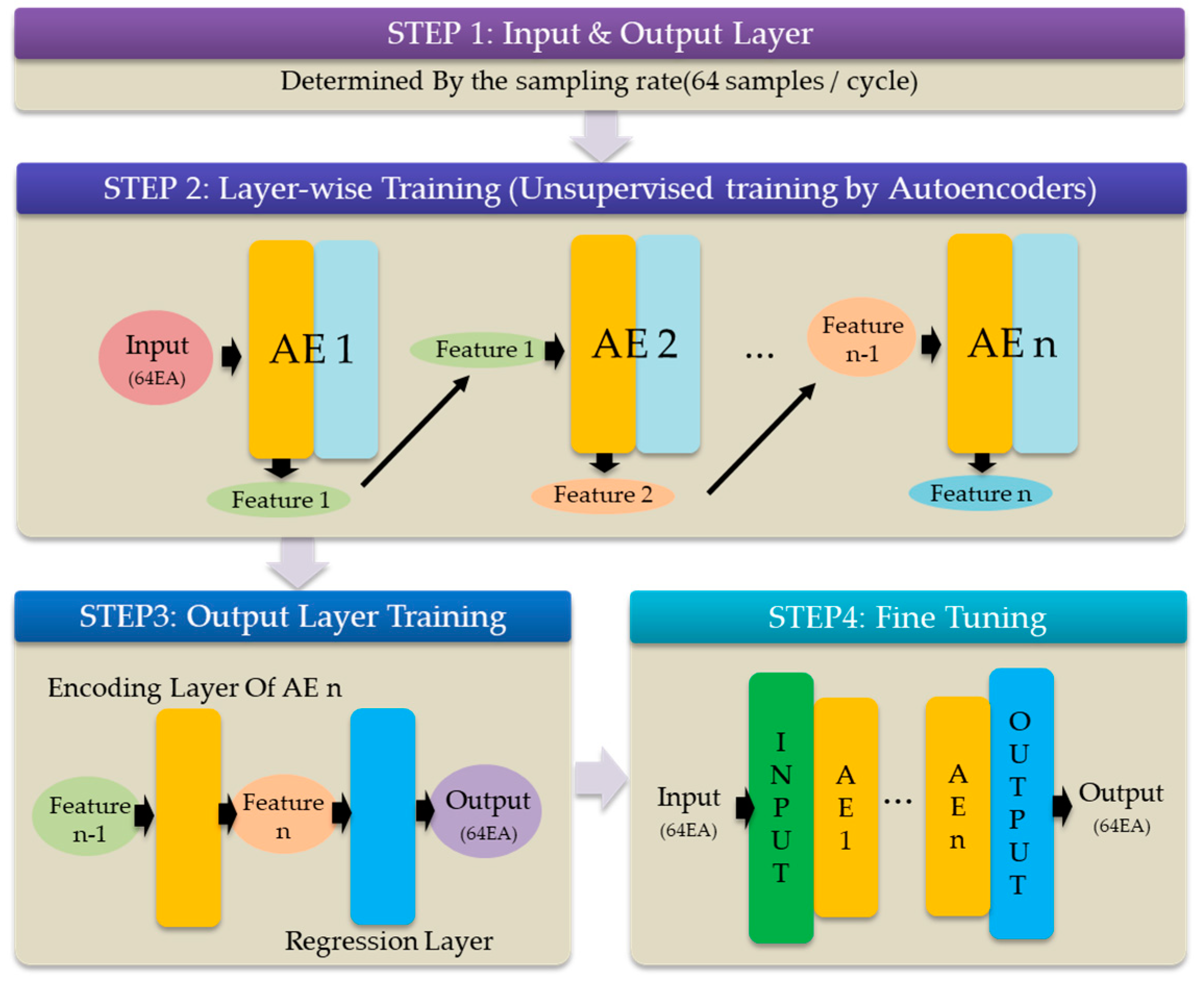
Figure 3 shows an overall process of the DNN training for this simulation. For every training step, the same cost function, optimizer, and training algorithm are utilized.

Figure 3.
Deep neural network (DNN) training process. AE—autoencoder.
Root mean square deviation (RMSD) is used as the cost function, as given in (4):
Among several optimizers offered in the TensorFlow library [31], the Adam optimizer was selected. This optimizer is a mixture of the RMSProp optimizer and the Momentum optimizer, which based on a general gradient descent (GD) algorithm. In the training loop, the RMSProp optimizer takes a different number of update values for each weight, which makes the training process more adaptive. This helps accelerate the training speed and refine the training process. The Momentum optimizer adds inertia to the weight update, to accelerate the convergence speed and allow the possibility of escape from bad local minima. The Adam optimizer is considered as one of the most efficient tools for achieving our purpose, as it combines the best features of both optimizers. The Adam optimizer is very effective, straight forward, requires little memory, is well suited for problems that are large in terms of data or parameters, and is appropriate for problems with noisy or sparse gradients [32].
3.2.1. Pre-Training Hidden Layers
Selecting a method to train hidden layers is significant for DNN. There are many techniques available such as an autoencoder, principal component analysis (PCA), missing values ratio, low variance filter, and others. However, the goal of this paper is to increase the accuracy of phase estimation, so the autoencoder is selected as it can replicate the structure of original data, and its performance is very accurate [33]. The key point regarding this process is the necessity of training an autoencoder sufficiently before moving on to the next autoencoder. If an autoencoder is not trained sufficiently, a certain amount of error would exist that would be delivered to the next autoencoder, causing cascading errors. In short, the pre-training is useless if the autoencoders are not properly trained. On this basis, we determined the number of neurons in hidden layers.
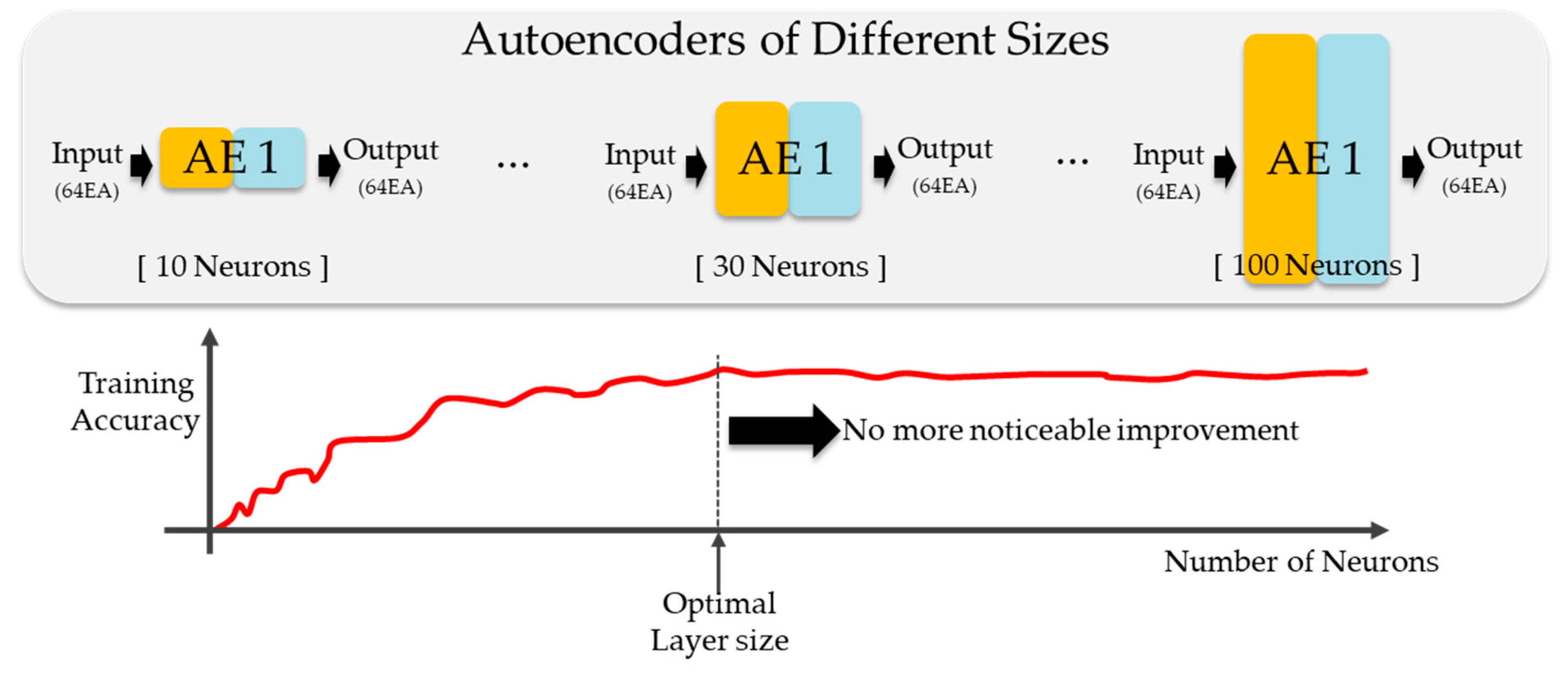
In layer-wise training shown in Figure 4, several autoencoders were implemented with different numbers of neurons. After training (unsupervised training using input as label), the training accuracy is compared to select the optimal size of the layer. Although more neurons give better performance in a neural network, there is a limit to the number of such neurons, beyond which the reconstructing performance of the autoencoder would not be improved further. In addition, the number of neurons in each layer may be different from the input size to prevent overfitting.

Figure 4.
Layer-wise training of a DNN using autoencoders to determine the optimal number of neurons in each layer (optimal layer size).
After the size of the first autoencoder is determined, the same procedure is repeated on the second autoencoder; the extracted features from the first autoencoder are used as an input. These steps are repeated several times until there is no further noticeable improvement in the reconstruction performance.
3.2.2. Pre-Training Output Layer
The output layer is known as the regression layer in this study, because we are performing regression through the DNN, not classification. Training an output layer is identical to training an autoencoder, except for the activation function. For an autoencoder, the ReLU function was used to reflect nonlinear characteristics in the extracted features. However, ReLU cannot be used as an activation function for the output layer, as ReLU only passes positive values and cannot express negative values. We aim to obtain a sinusoidal current waveform containing negative values, from the output layer; thus, the output layer was set as a linear layer, meaning that it has no activation function. By setting the output layer as a linear layer, it becomes possible to express negative values, and training can proceed. As the signal without interference (DC offset, harmonics, and noise) was used as a label, the training process of the output layer is supervised.
3.2.3. Supervised Fine Tuning
DNN training includes the input layer, hidden layers, and output layer. After completing the pre-training of each layer, every layer is stacked together. To improve the performance of the DNN, it is necessary to connect the pre-trained layers naturally, and to adjust the pre-trained weights precisely while taking every layer into account. The DNN is optimized using this process, which is called supervised fine tuning.
3.3. Determination of the DNN Size
To determine the DNN size including the number of neurons in each layer and the number of hidden layers, we used partial datasets instead of the whole datasets, because using 9,545,040 datasets would be time-consuming and ineffective and, as the purpose of this step is investigation of the reconstruction ability of autoencoders with different sizes, there would be no issue in using partial datasets. The validation datasets were used as the partial datasets to determine the DNN size.
The DNN size was decided according to an experimental procedure based on applying the training process repeatedly. We implemented DNNs with different numbers of hidden layers, so that we could determine the optimal number of layers by analyzing the training results, similar to the determination of the number of neurons in each layer. After completing the determination of the DNN size, we re-initialized all weights before the pre-training process.
3.3.1. Number of Neurons in Each Layer
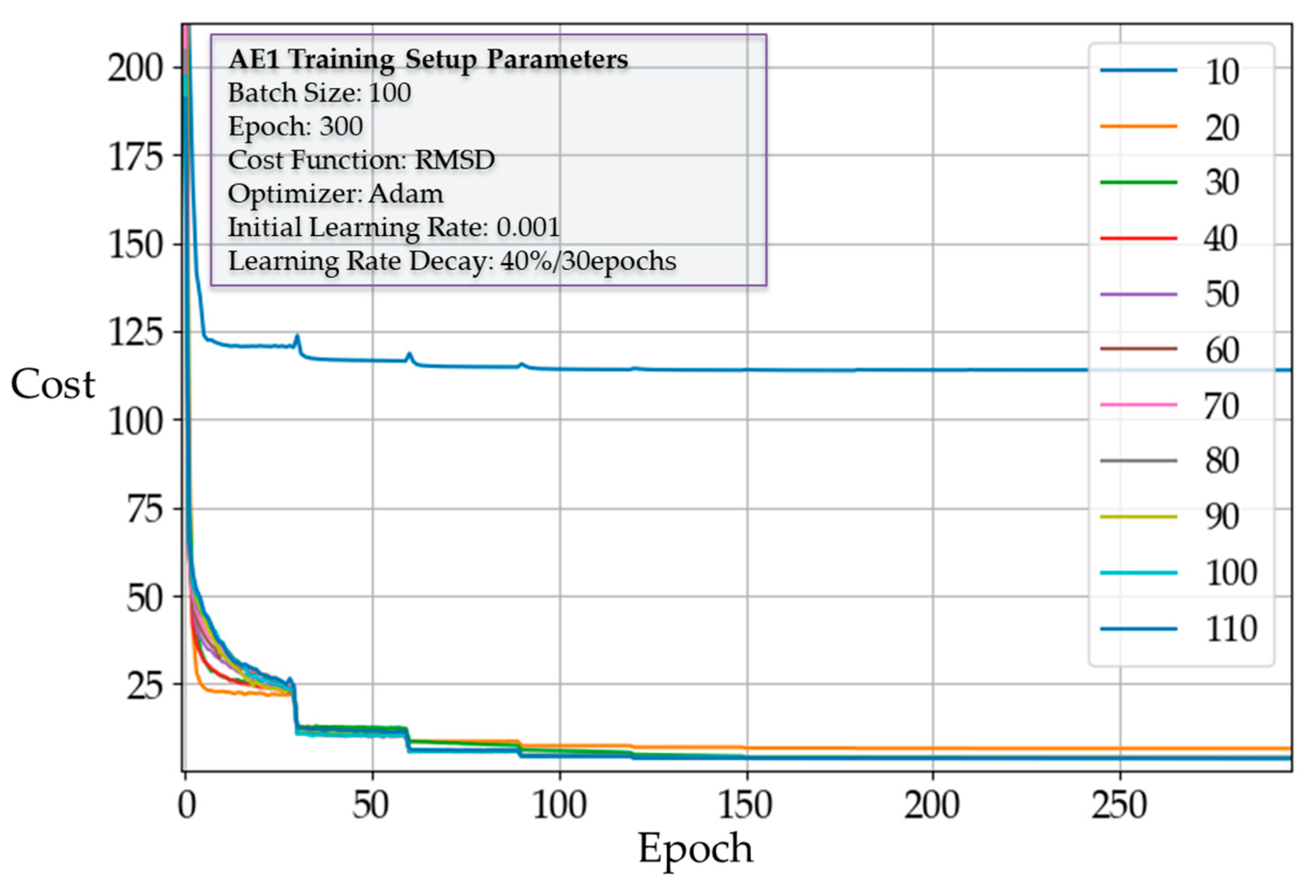
As described in Section 3.2.1, for the first hidden layer, we implemented autoencoders with a different number of neurons and recorded the average cost of each epoch during training. For the first hidden layer, we implemented autoencoders with different sizes and recorded the average cost of each epoch during training. Figure 5 shows the effect of the number of neurons on the cost reduction. In every case, regardless of the number of neurons, there was no significant change in cost after about 150 epochs. However, the point of convergence differed depending on the size. In fact, except for sizes 10 and 20, every other case converged to a similar cost value. This implies that 30 neurons may be an adequate number for AE1. To confirm this, we analyzed the training accuracy of each case by calculating the maximum cost, average cost, and its standard deviation. Figure 6 and Figure 7 show the waveforms corresponding to the maximum RMSD for different sizes of AE1. The results of experimental training for AE1 are summarized in Table 3. From the cost reduction curve shown in Figure 5, we expected that AE1 with 30 neurons would be optimal. However, from the RMSD analysis given in Table 3, it was found that AE1 with 50 neurons would be optimal. With more than 40 neurons, the RMSD started to fall within the acceptable range.
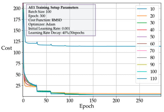
Figure 5.
Cost reduction curve of autoencoder 1 (AE1) with different sizes. RMSD—root mean square deviation.
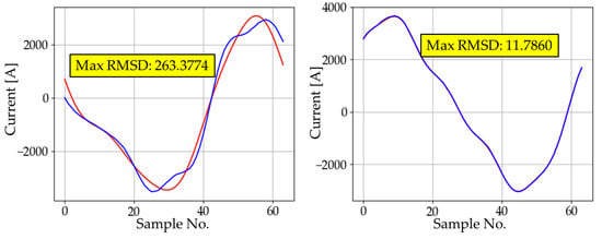
Figure 6.
The waveform with the maximum RMSD for different sizes of AE1.
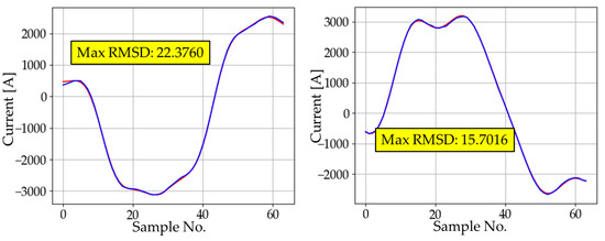
Figure 7.
The waveform with the maximum RMSD for different sizes of AE1.

Table 3.
Root mean square deviation (RMSD) analysis (autoencoder 1 (AE1)).
This result implies that the performance of the autoencoder does not depend entirely on the final cost of training. Among the eight candidates that fall within the desired range of RMSD, 50 neurons are chosen as the size of AE1 because of a desire to spare neurons for AE1 in order to simulate partial datasets rather than the whole datasets.
As the size of AE1 was determined to be 50, the size of the first hidden layer of the DNN would also be 50. This is the entire procedure for deciding the hidden layer size. We performed three more experiments under the same scenario to determine the size of the next hidden layers and determined the size of hidden layers as follows: Hidden layer 1:50, Hidden layer 2:50, Hidden layer 3:60, and Hidden layer 4:50.
3.3.2. Number of Hidden Layers
After the four different sizes of DNNs in TensorFlow are implemented, as shown in Figure 8, each output layer is trained before performing the fine tuning.

Figure 8.
Four DNNs with different numbers of hidden layers.
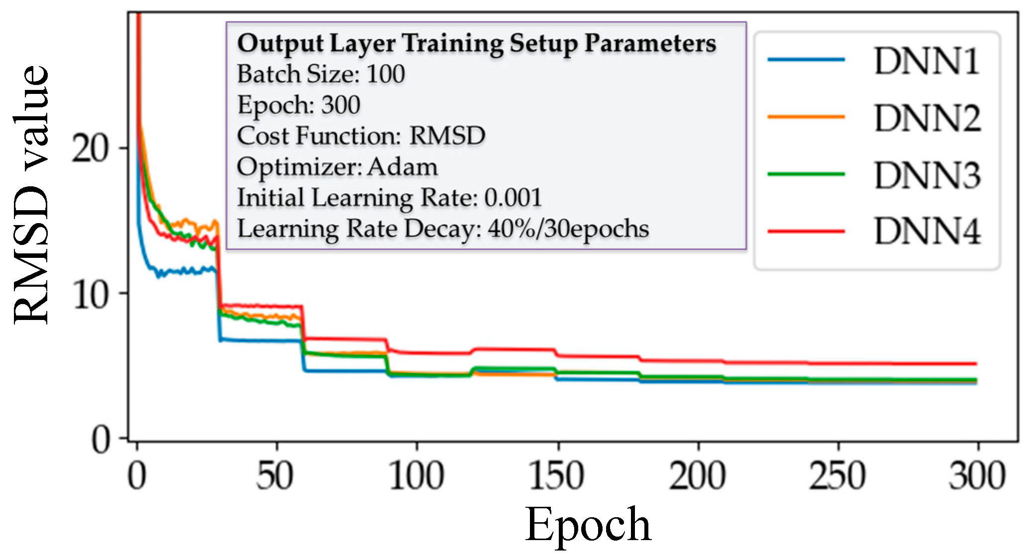
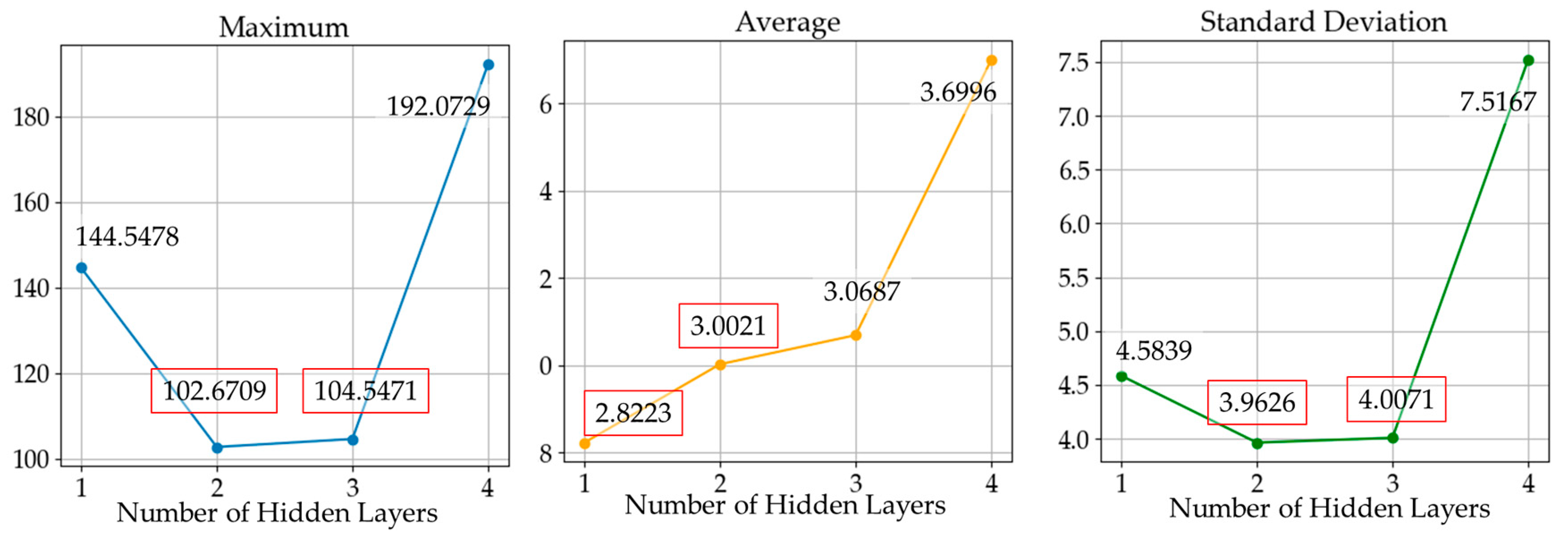
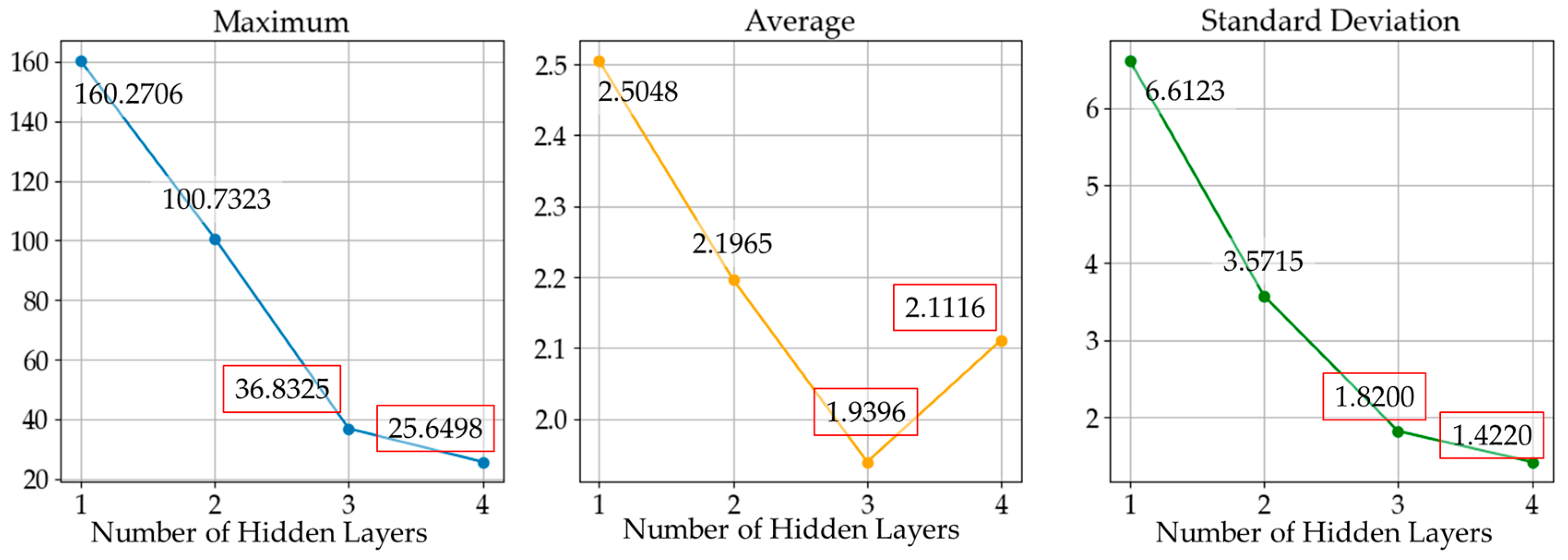
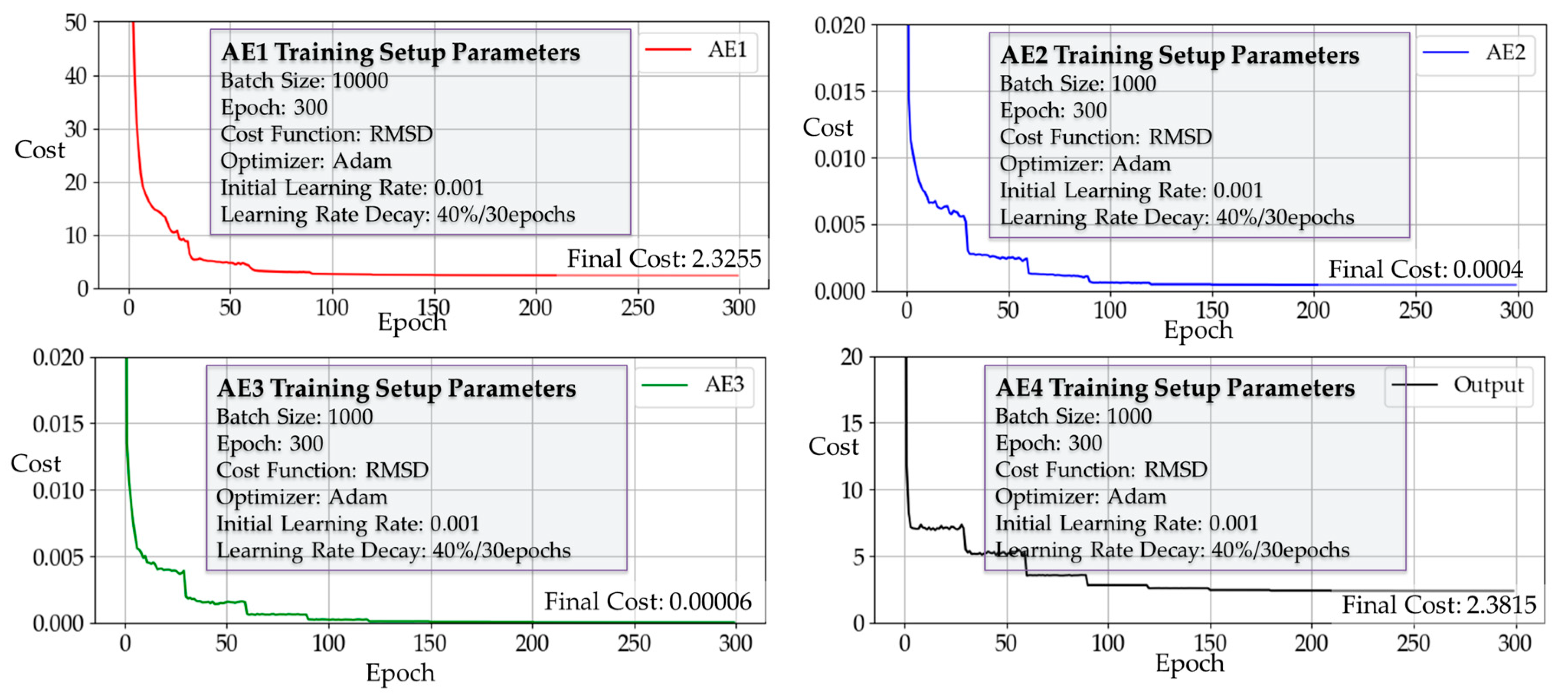
The training process of the output layer was performed by the layer-wise training method, and the training parameters and the training results for each output layer are shown in Figure 9. Every DNN except DNN4 showed a similar training performance regarding the cost reduction. For more precise comparison between different numbers of hidden layers, we performed RMSD analysis, and the results are shown in Figure 10. In Figure 10, DNN1 had the lowest average RMSD; however, DNN2 and DNN3 performed better in terms of the maximum and standard deviation error. DNN4 showed the worst performance, even though it had the most hidden layers.
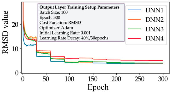
Figure 9.
Four DNNs with different numbers of hidden layers.
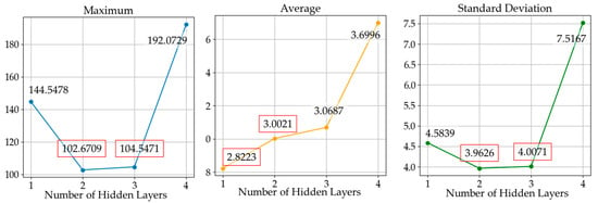
Figure 10.
Maximum, average, and standard deviation of costs depending on the number of hidden layers after output layer training; the two cases with the best performance are marked in red.
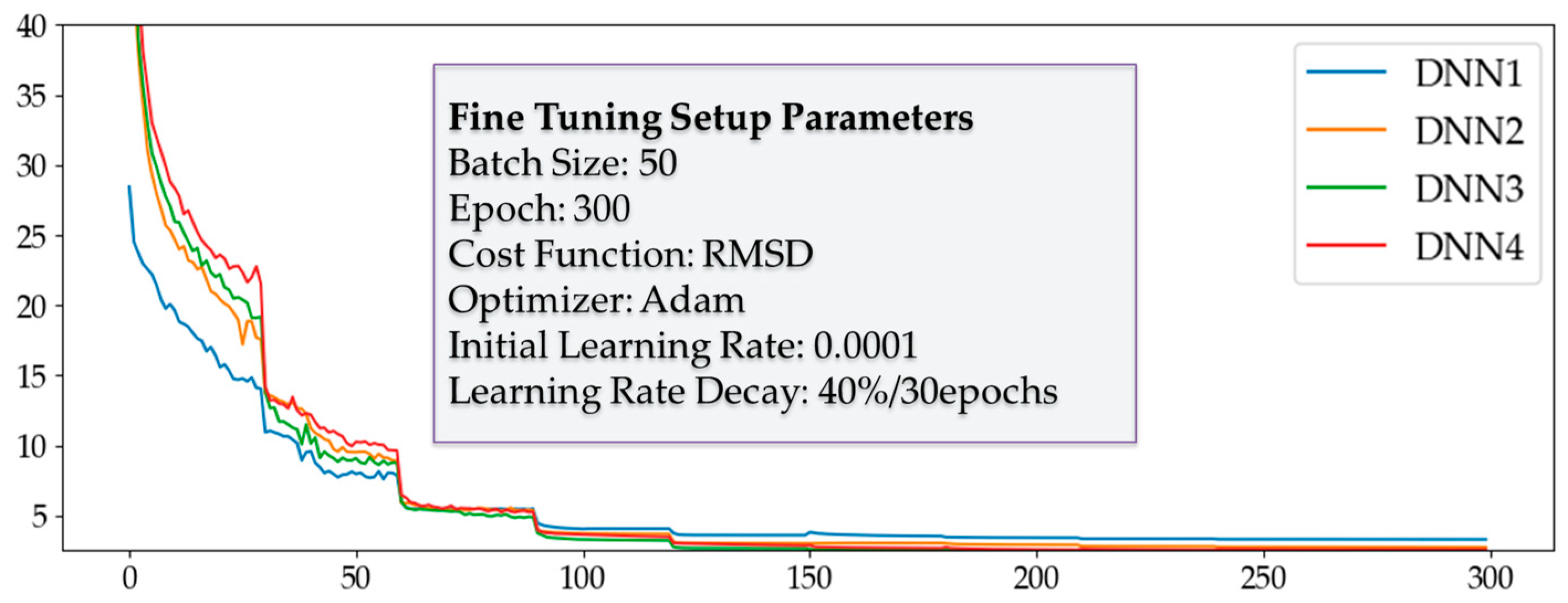
Fine tuning was then conducted to confirm the best-performing DNN. Unlike the layer-wise training, fine tuning is a training process that involves all layers of the DNN; thus, we connected every layer in the DNNs, as shown in Figure 8. The results of the fine tuning are shown in Figure 11 and Figure 12. The results of RMSD analysis after fine tuning were significantly different to those from before. In the results before fine tuning, the performance of DNN appeared to be independent of the number of hidden layers. However, comparing the results after fine tuning, the maximum and standard deviation error appeared to decrease as the number of hidden layers increased; DNN3 and DNN4 were within an acceptable range of error. Finally, DNN3 was chosen because it performed best in terms of the average error and has the simplest structure capable of obtaining the desired accuracy.
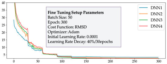
Figure 11.
Cost reduction curve of four DNNs with different numbers of nodes after fine tuning.
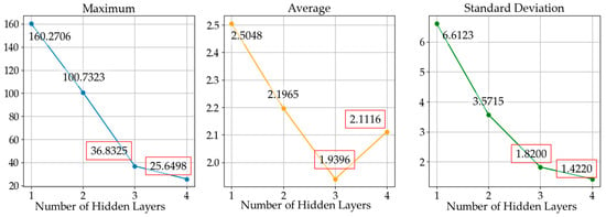
Figure 12.
Maximum, average, and standard deviation of costs depending on the number of hidden layers after fine tuning; the two cases with the best performance are marked in red.
3.4. DNN3 Training Result
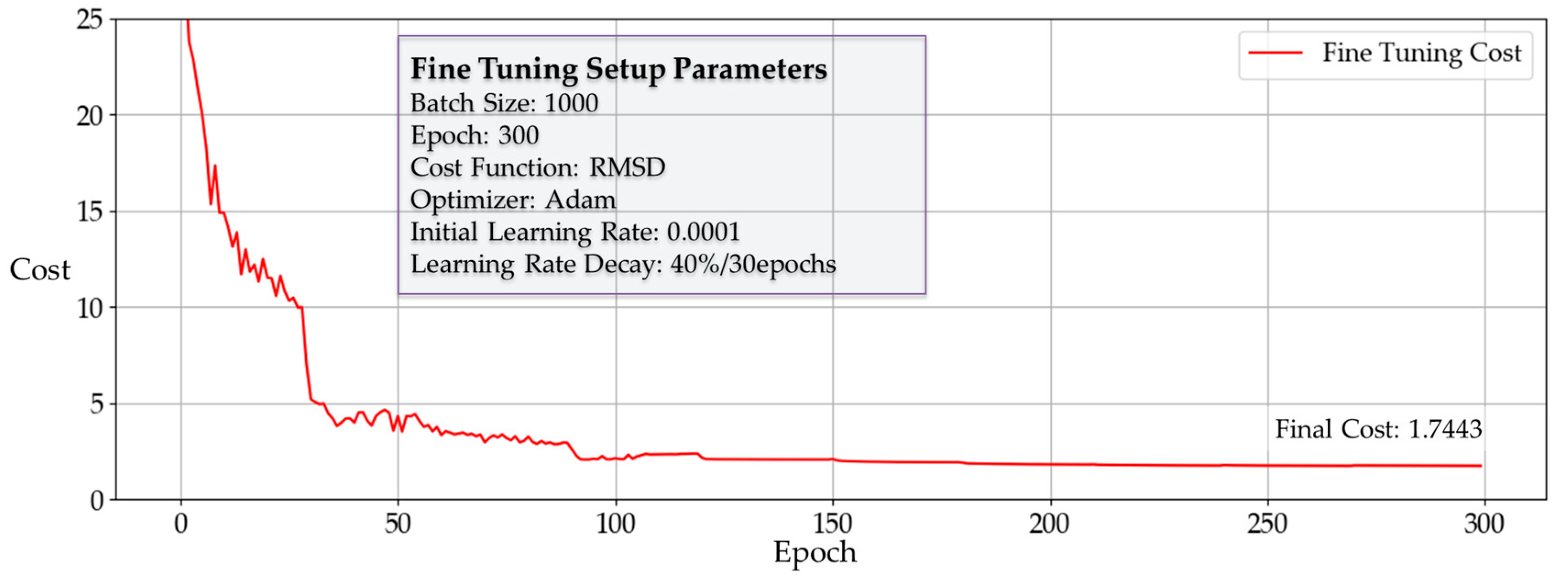
Figure 13 shows the cost reduction curves of three autoencoders and the output layer, and Figure 14 shows the cost reduction curve of fine tuning. Comparing the average cost between the layer-wise trained DNN and the fine-tuned DNN3, the latter exhibited a lower final average cost. This demonstrates the effectiveness of the fine-tuning step for improving performance.

Figure 13.
Cost reduction curves of three autoencoders and the output layer.
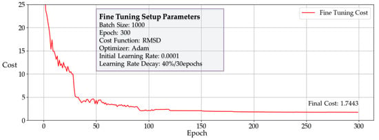
Figure 14.
Cost reduction curve of DNN3 fine-tuning stage.
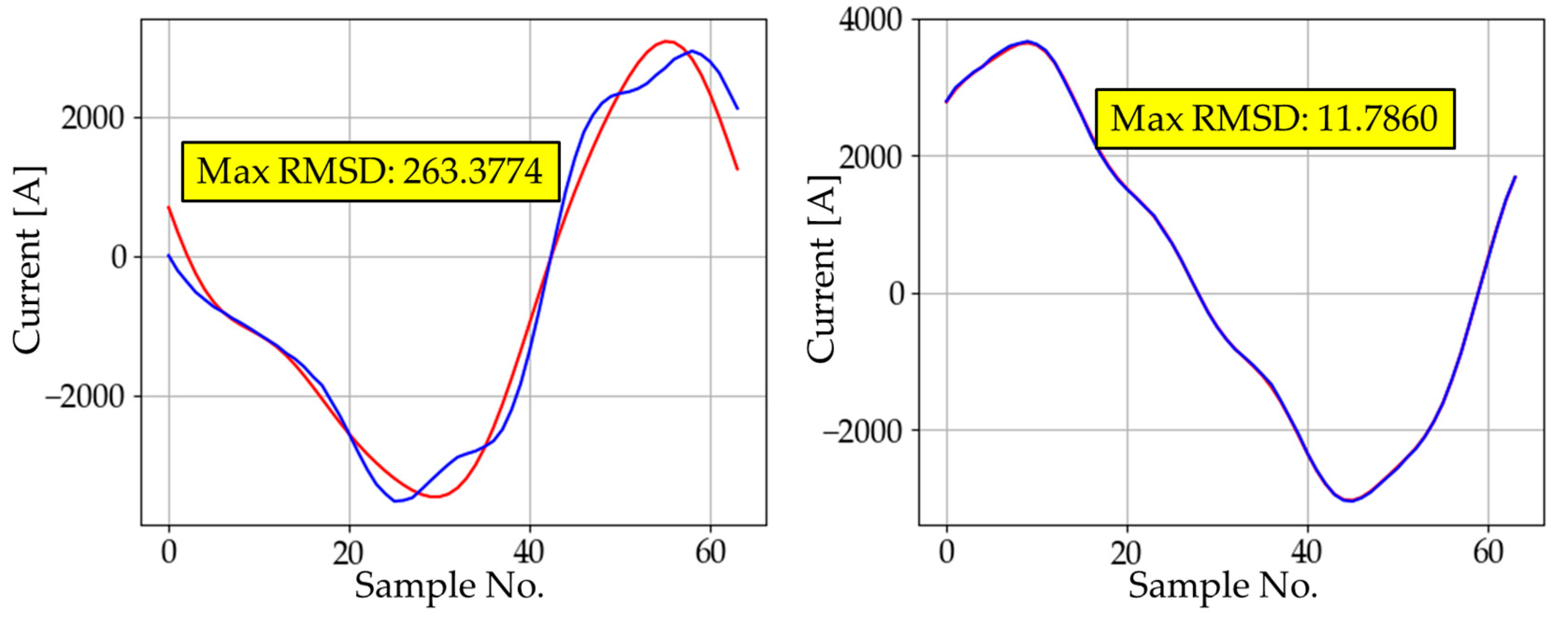
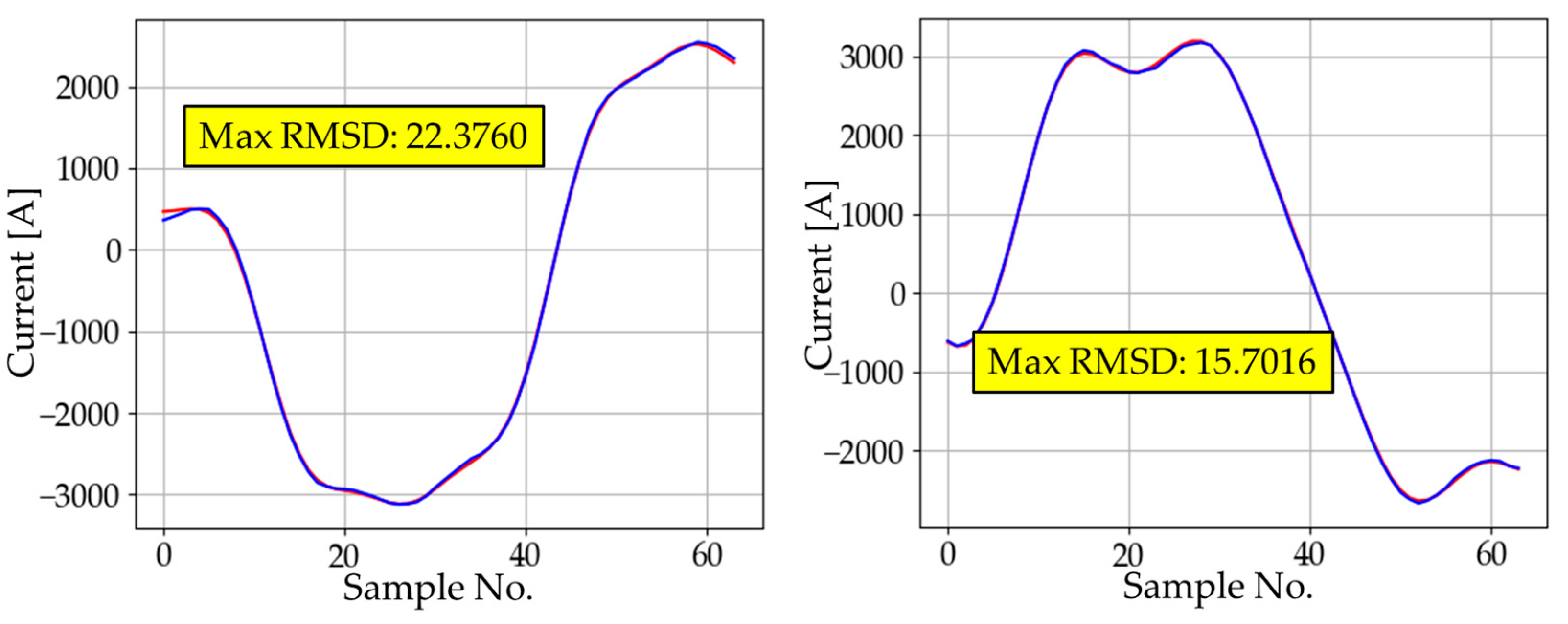
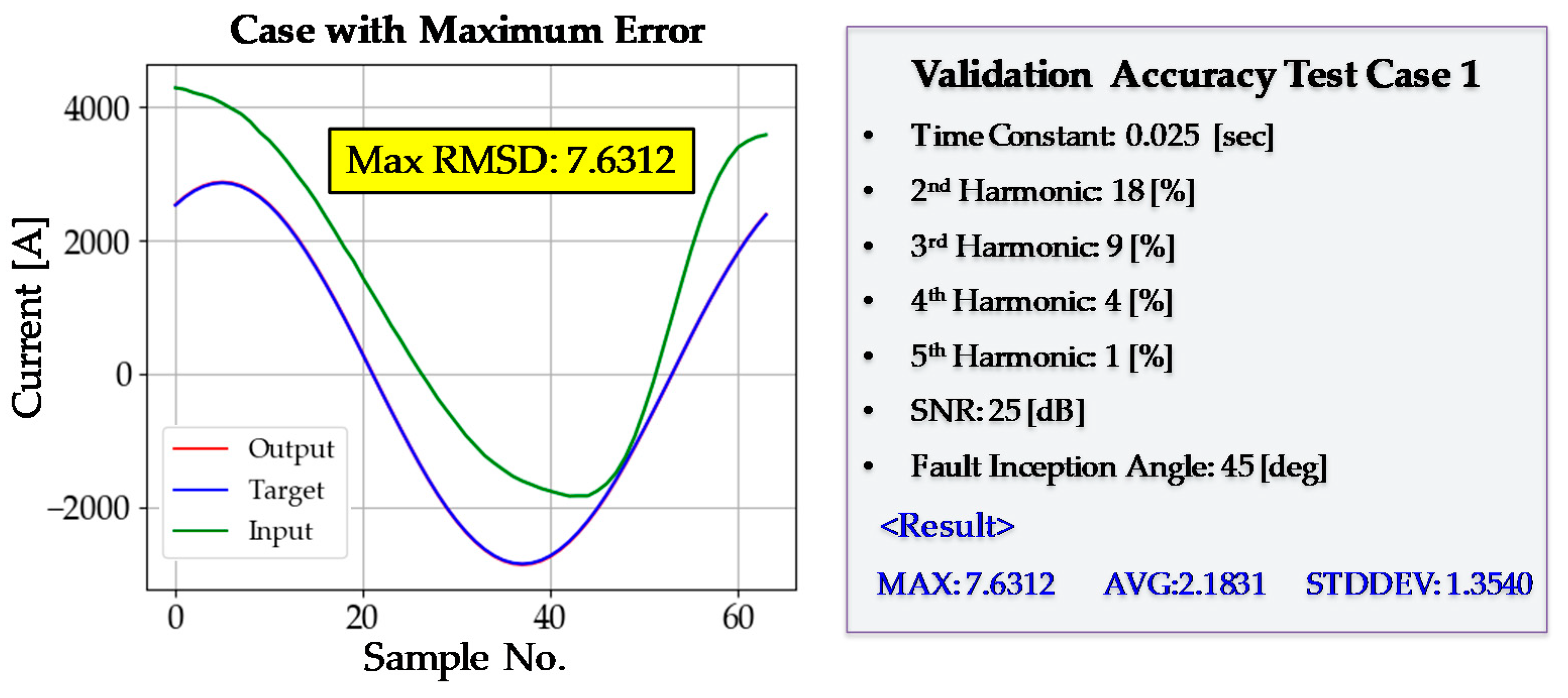
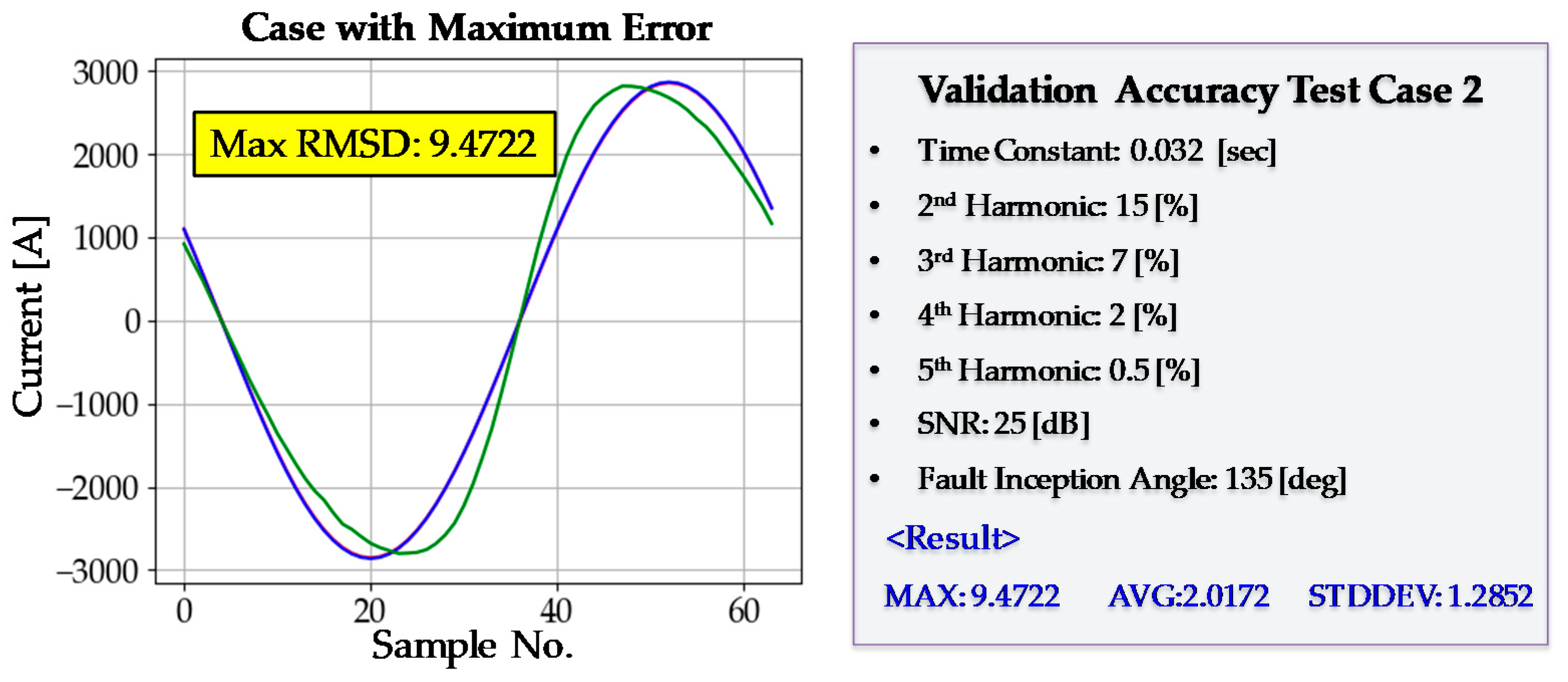
After every training step had been completed, a validation test was performed. The purpose of the validation test was to examine the generality of the DNN3. Even if the training is conducted successfully, the DNN3 may not operate accurately in new situations it has not experienced before, a phenomenon known as overfitting. The maximum, average, and standard deviation of the RMSD were 11.3786, 2.1417, and 1.3150, respectively; there was no sign of overfitting. The average value of RMSD was low, and the standard deviation was also sufficiently low. A more detailed analysis of validation accuracy is provided in Figure 15 and Figure 16. The DNN3 shows good accuracy even in situations that have not been experienced before in the training process. Finally, the training process of DNN3 was considered to have been completed successfully.

Figure 15.
Validation test case 1. SNR—signal-to-noise ratio.
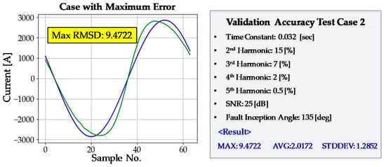
Figure 16.
Validation test case 2.
4. Performance Tests and Discussions
PSCAD/EMTDC is used to model the power system shown in Figure 17 and generate datasets for performance testing.

Figure 17.
Power system model for test datasets (PSCAD/EMTDC).
After modeling was completed, single line to ground faults were simulated to acquire fault current waveforms with DC offset. By adding harmonic components and additive noise, we were able to prepare test datasets that can verify the performance of the DNN3. For a comparative analysis between the proposed DNN3 and digital filtering algorithms, we implemented a second order Butterworth filter and a mimic filter (known as a DC-offset filter), which is commonly used in the existing digital distance relays [34]. Even if the noise component is removed using an analog low-pass filter before ADC, the influence of the noise generated after the ADC cannot be eliminated from the current waveform. We have taken this into account while generating the test datasets.
4.1. Response to Curents without Harmonics and Noise
In this test, the current waveform includes only the fundamental current and the DC offset. Regarding the DC offset, three cases were considered: DC offset in a positive direction, DC offset in a negative direction, and a relatively small amount of DC offset.
4.1.1. Instantaneous Current
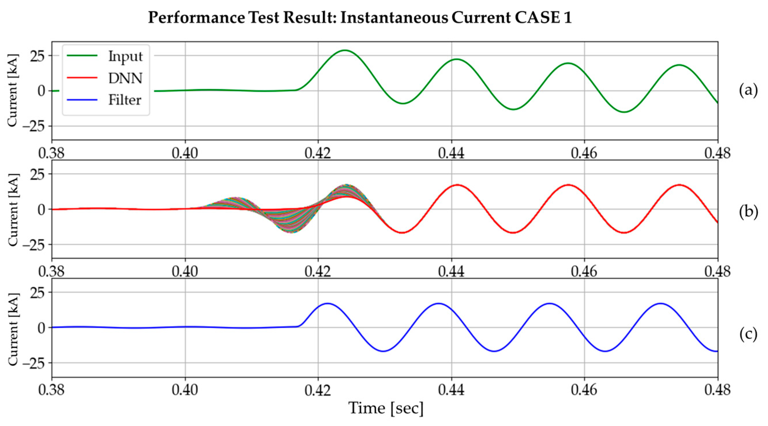
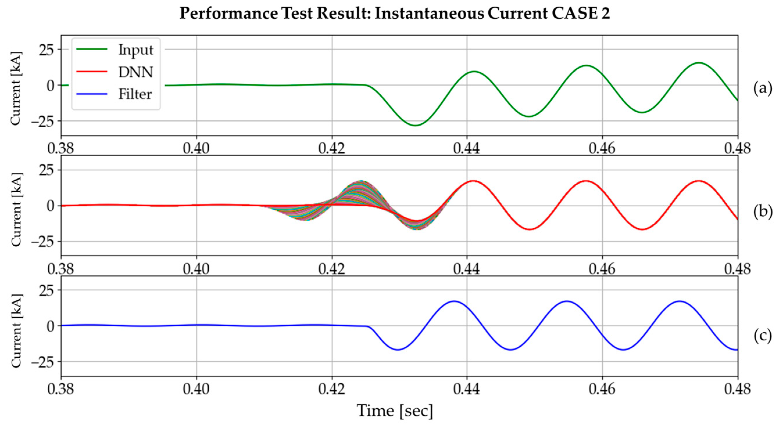
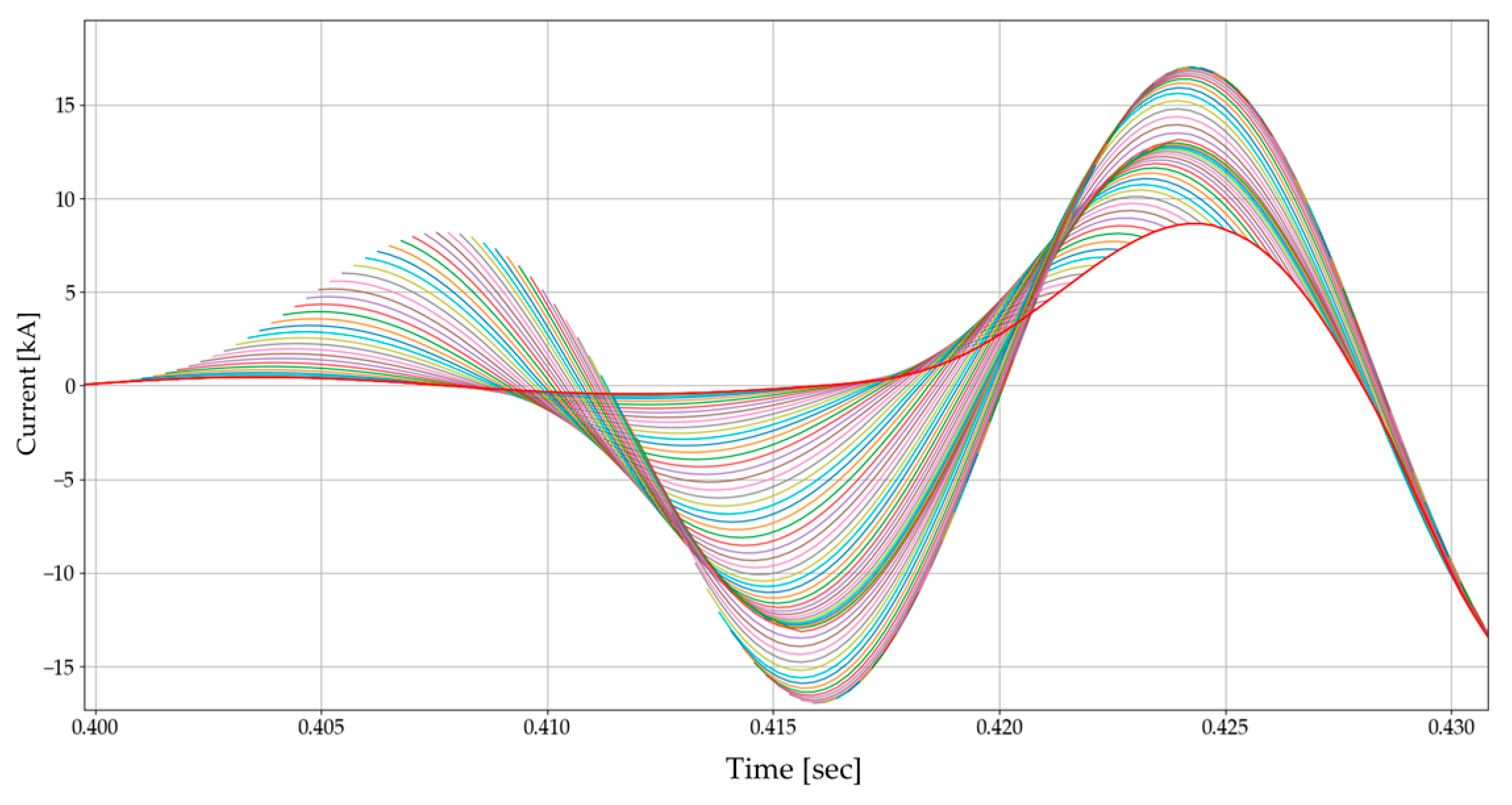
Figure 18 and Figure 19 show the input, DNN3 output, and DC-offset filter output for three different cases. Every DNN3 output (size of 64) overlaps in the graph, and this demonstrates the distinct features of the DNN3 output. As the DNN3 had no opportunity to be trained for transient states, it exhibits unusual behavior near the fault inception time. However, subsequent tests have confirmed that this phenomenon has no adverse effect on the phasor estimation process, based on full-cycle discrete Fourier transform (DFT). As the output of the DNN3 is in the form of a data window, we plotted the most recent values using a red line, as shown in Figure 20. From this point forwards, the instantaneous current value will be plotted in this way.
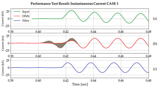
Figure 18.
Performance test result on DC offset in the positive direction (time constant: 0.0210 s, fault inception angle: 0°): (a) input current signal; (b) DNN3 output; (c) DC-offset filter output.
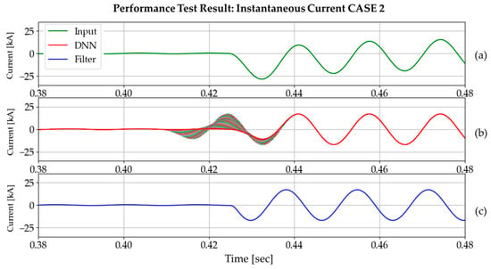
Figure 19.
Performance test result on DC offset in the negative direction (time constant: 0.0210 s, fault inception angle: 180°): (a) input current signal; (b) DNN3 output; (c) DC-offset filter output.
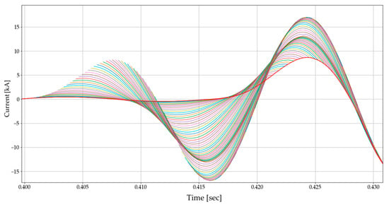
Figure 20.
DNN3 response to the transient state.
4.1.2. Results and Comparisons of Instantaneous Current
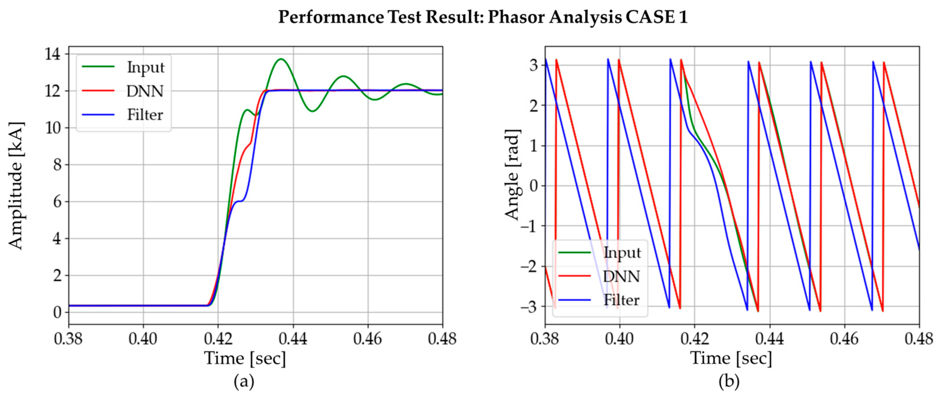
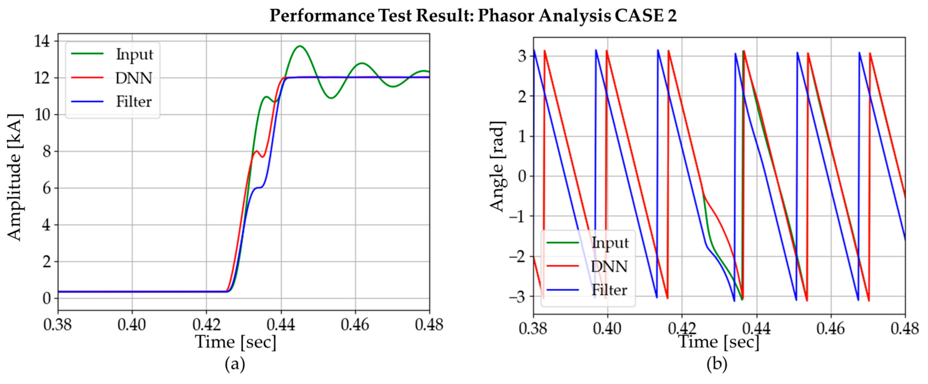
Figure 21 and Figure 22 show the phasor analysis results for two different cases. Original signal (green waveform), signal after using DNN (red waveform), and signal after using DC-offset filter (blue waveform) in Figure 19 are used to simulate their performances using the full-cycle DFT algorithm.

Figure 21.
Comparison of phasor estimation between DNN3 output and DC-offset filter output: CASE 1.
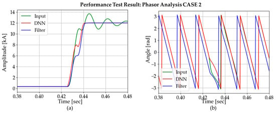
Figure 22.
Comparison of phasor estimation between DNN3 output and DC-offset filter output: CASE 2.
While applying DFT to the three signals, the DNN signal gave the fastest convergence speed. Table 4 summarizes the amplitude convergence time for each method in three different cases. According to the table, the DNN method has the best convergence time for all cases studied.

Table 4.
Amplitude convergence time [ms]. DNN—deep neural network.
4.1.3. Comparison Using Inaccurate Time Constants
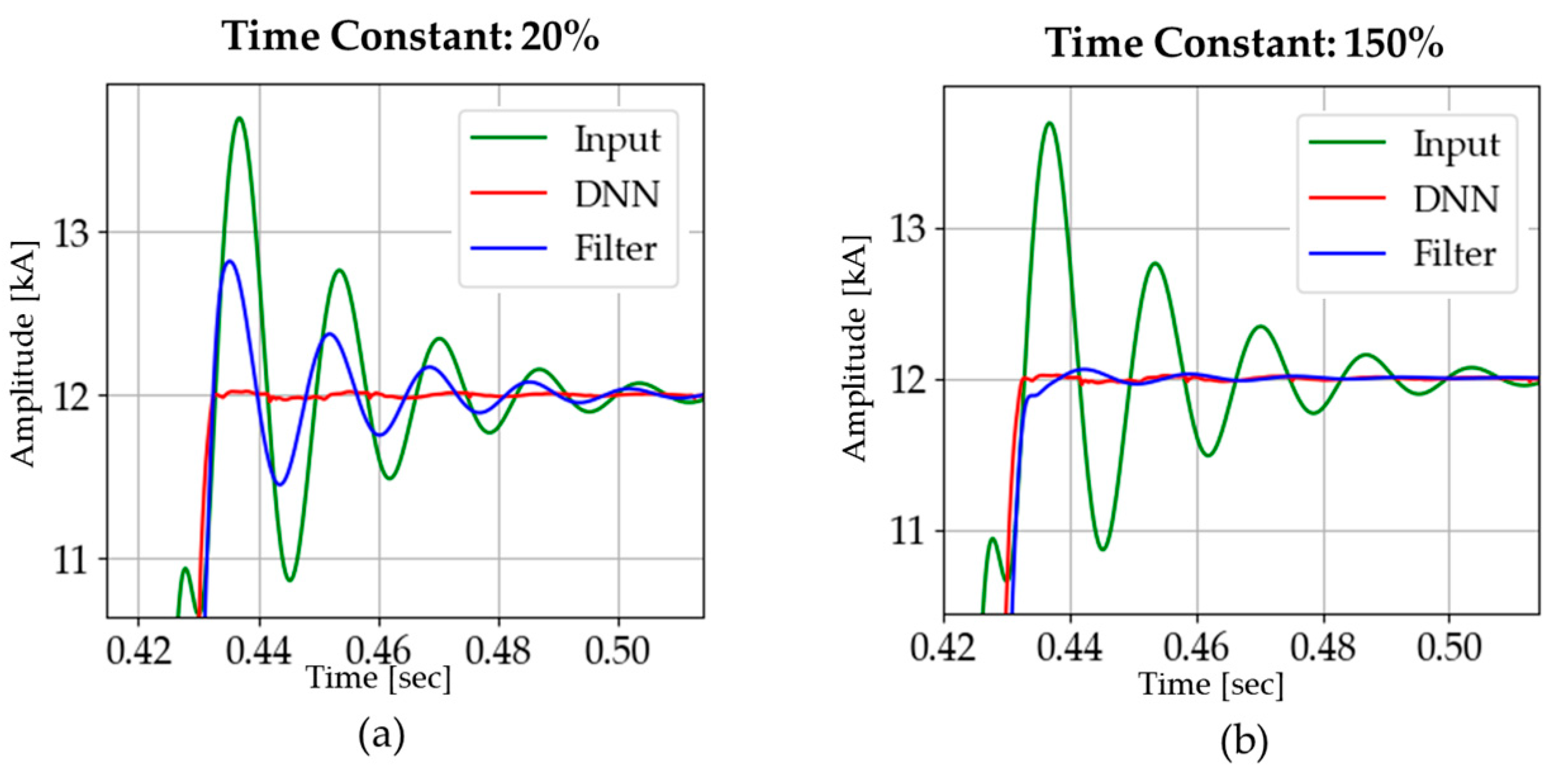
We have discussed the test results in the case in which the time constant is predicted accurately; however, when an inaccurate time constant is used in a DC-offset filter, its performance is adversely affected, as shown in Figure 23.
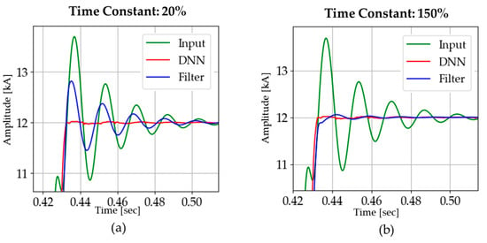
Figure 23.
Phasor estimation with inaccurate time constants (the accurate time constant of 0.0210 s): (a) 20%: 0.0042 s; (b) 150%: 0.0315 s.
In the case of the DC-offset filter, some oscillations appear in the current amplitude after fault inception depending on the extent of the inaccuracy in the time constant. On the other hand, the DNN shows robust characteristics and has less convergence time.
4.2. Case Study
For further performance analysis of the proposed DNN3, we will discuss three case studies in this section.
4.2.1. Case A (Line to Line Fault)
Up to this point, we have performed tests based only on the single line to ground fault simulated by PSCAD/EMTDC. In this case, the fault type is changed to a line to line fault. In addition, harmonics and noise are considered simultaneously.
- Voltage level: 154 kV
- Time constant: 0.0210 s
- Harmonics: 2nd = 11%, 3rd = 7%, 4th = 3%, 5th = 0.5%
- Noise: 25 dB
- Fault type: line to line fault (phase A and phase B short circuit)
- Fault inception angle: 30°
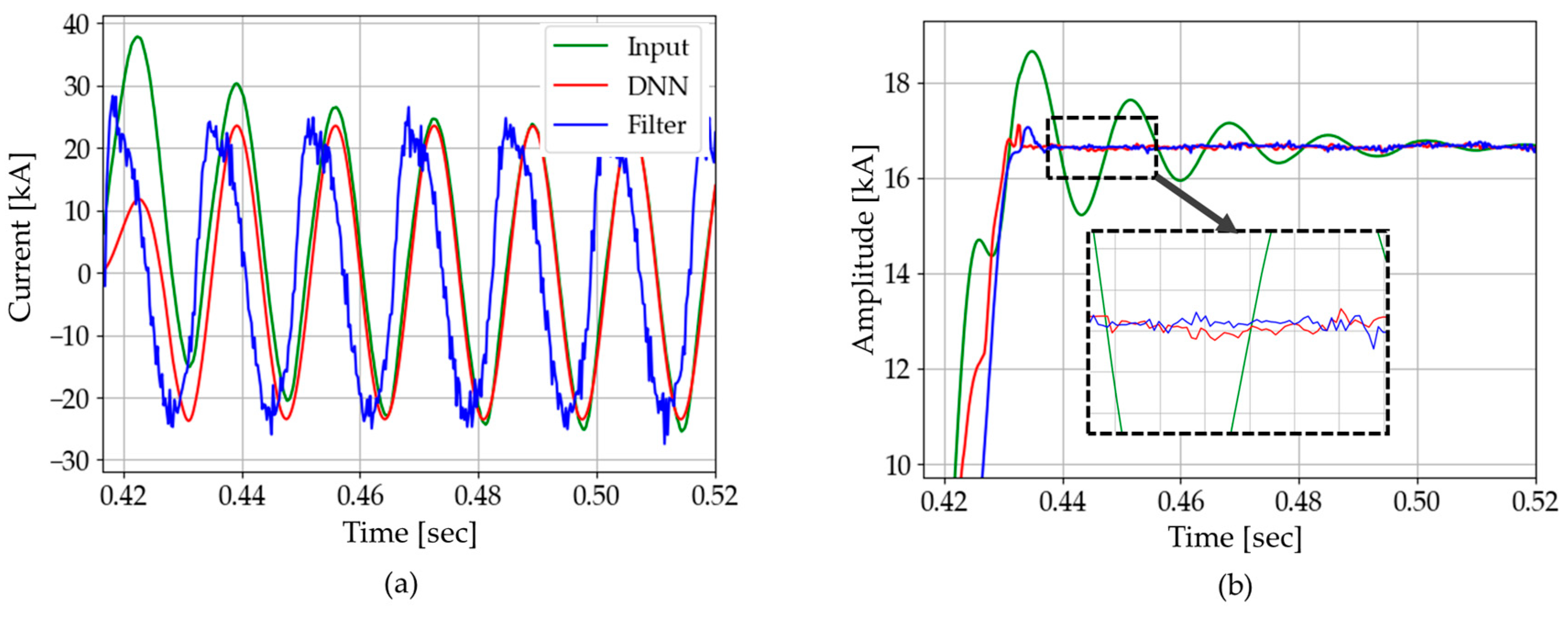
Figure 24 shows the test results of CASE A, which are summarized in Table 5. DNN3 has a faster convergence speed and lower standard deviation compared with the DC-offset filter. Compared with the original input (where DC offset was not removed), the DC-offset filter shows remarkable improvement, though it still performs slightly less effectively than the DNN3. However, Figure 24a shows at a glance that the performance of the DC-offset filter is very poor in estimating the instantaneous current waveform. As a result, it was found that the DNN3 performed much better, even though the test was conducted with the DC-offset filter given a precise time constant. Thus, in the case of line to line fault, the proposed method is better than the DC-offset filter in both factors, convergence time and standard deviation.
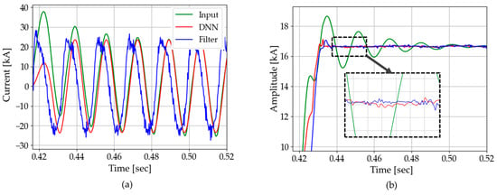
Figure 24.
Test results of CASE A: (a) instantaneous current; (b) amplitude.

Table 5.
Case A: analysis of current amplitude (phasor).
4.2.2. Case B (Different Power System Situation)
To verify the generality of the proposed DNN3, we performed a test using a fault current in a different power system model.
- Voltage level: 22.9 kV
- Time constant: 0.0402 s
- Harmonics: 2nd = 18%, 3rd = 12%, 4th = 8%, 5th = 4%
- Noise: 25 dB
- Fault type: single line to ground fault
- Fault inception angle: 0°
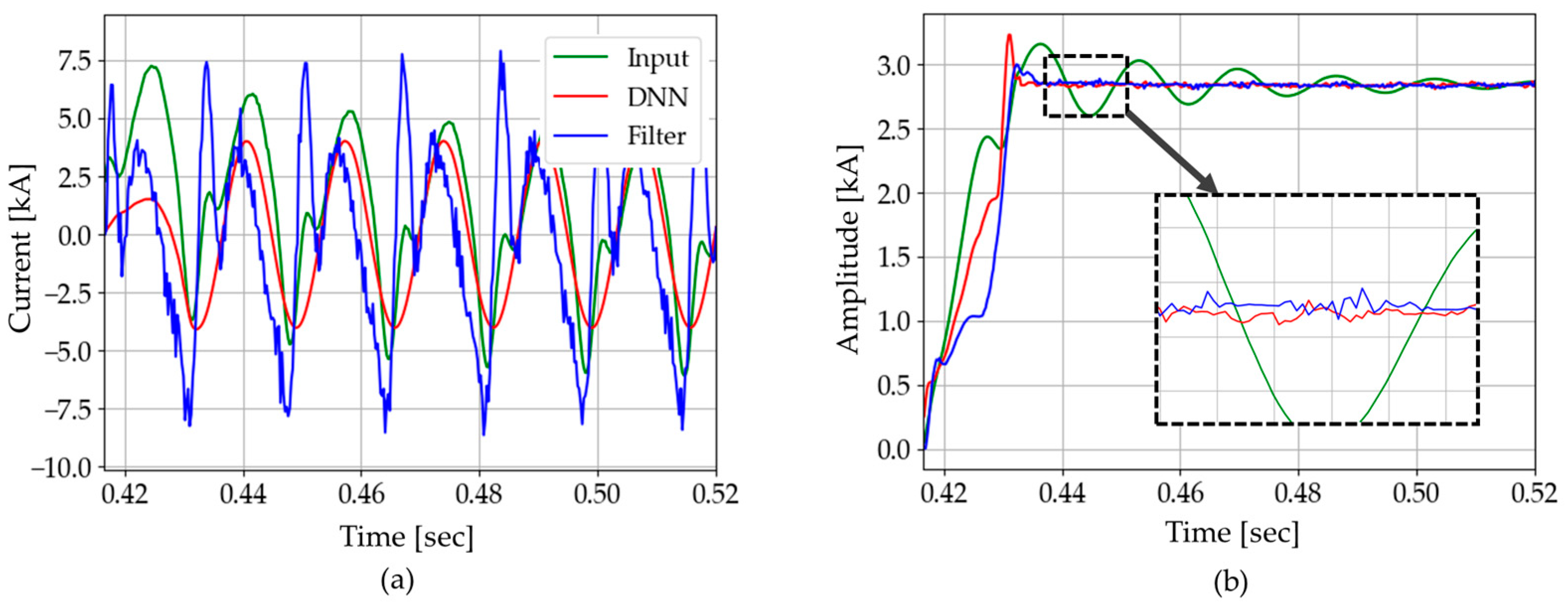
The generality of the proposed DNN3 is verified through this test, as the results are close to those of CASE A, as shown in Figure 25 and summarized in Table 6. Even under the increased level of harmonics, as compared with former test cases, DNN3 exhibited robust performance with less convergence time and lower standard deviation, while a different power system model is used for the simulations.

Figure 25.
Test results of CASE B: (a) instantaneous current; (b) amplitude.

Table 6.
Case B: analysis of current amplitude (phasor).
4.2.3. Case C (Different Power System Situation)
In this section, we have observed how the proposed DNN3 and the DC-offset filter responded to the presence of fault resistance. The details of the studied system are given bellow:
- Voltage level: 345 kV
- Time constant: 0.034 s
- Harmonics: 2nd = 12%, 3rd = 4%, 4th = 2%, 5th = 0.2%
- Noise: 25 dB
- Fault type: single line to ground fault (fault resistance 1 ohm)
- Fault inception angle: 0°
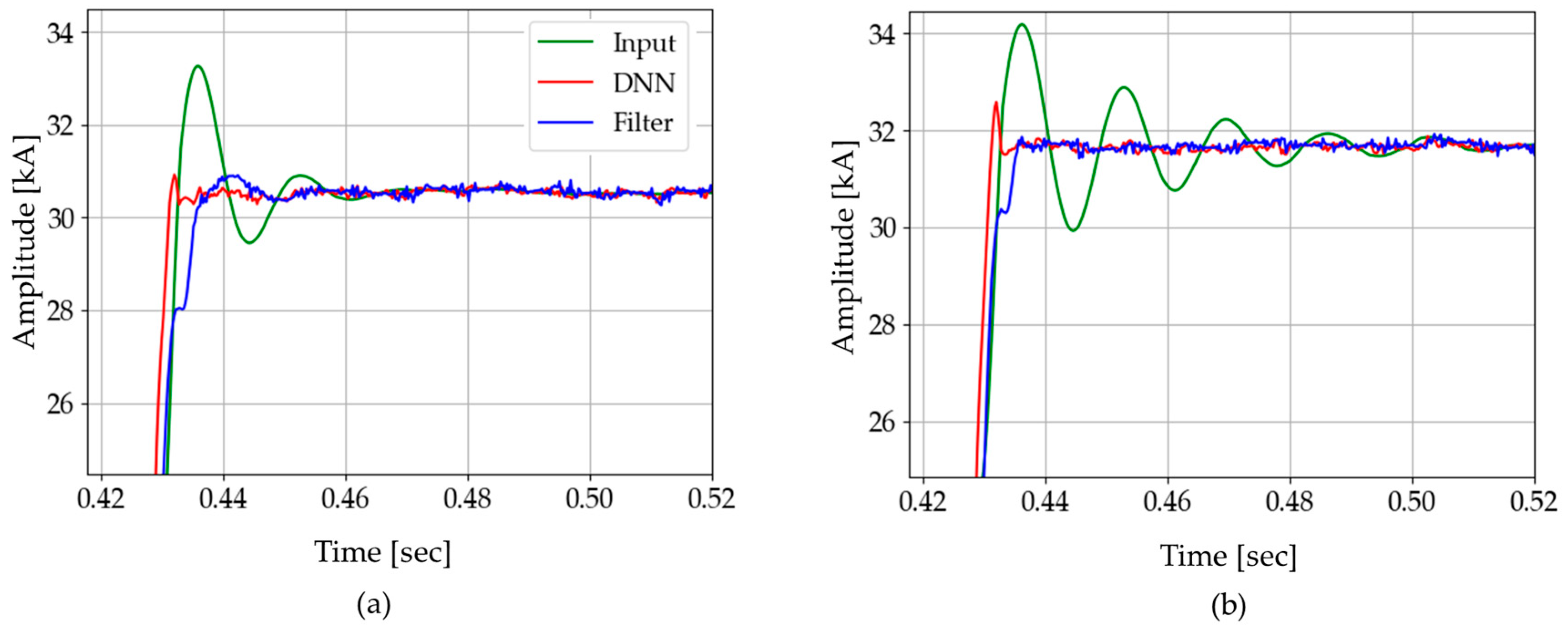
In Figure 26a, it is seen that the oscillations appear in the result of the DC-offset filter when a fault resistance exists. This oscillation is caused by the fault resistance, which affects the time constant of the DC offset. As summarized in Table 7, the oscillation had an adverse effect on the convergence time of the filter. In contrast, DNN3 was not influenced by the fault resistance, which has shown its potential to solve this problem.
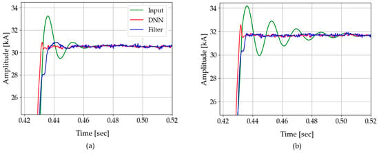
Figure 26.
Test results of CASE C: comparison between two cases: (a) fault resistance: 1 Ω; (b) no fault resistance.

Table 7.
Case C: analysis of current amplitude (phasor).
5. Conclusions
In this paper, we developed a DNN to effectively remove DC offset. Autoencoders were used to determine the optimal size of the DNN. Subsequently, intensive training for the DNN was performed using both the supervised and unsupervised training methodologies.
Even under harmonics and noise distortion, the DNN showed good and robust accuracy in instantaneous current reconstruction and phasor estimation, compared with the DC-offset filter. It was also confirmed that the errors due to inaccurate time constants of the DC offset were significantly reduced compared with the DC-offset filter. These results confirmed that the method of determining the DNN size using the autoencoder was appropriate. Therefore, the optimal DNN size in other deep learning applications could be determined based on this methodology. As the performance of the DNN is largely affected by the quality of the training datasets, it would be possible to train the DNN more precisely if more sophisticated training datasets could be prepared.
Furthermore, it is expected that it would be possible to reconstruct the secondary current waveform of the current transformer distorted by saturation, by modeling the current transformer mathematically and applying the methodology used in this paper.
Author Contributions
S-B.K. prepared the manuscript and completed the simulations. S-R.N. supervised the study and coordinated the main theme of this paper. V.S. developed the simulation model in the study and revised the manuscript. S-H.K. and N-H.L. discussed the results and implications, and commented on the manuscript. All of the authors read and approved the final manuscript.
Funding
This research was supported in part by the Human Resources Program in Energy Technology of the Korea Institute of Energy Technology Evaluation and Planning (KETEP), and granted financial resources from the Ministry of Trade, Industry & Energy, Republic of Korea (No. 20154030200770). This research was also supported in part by Korea Electric Power Corporation (Grant number: R17XA05-2).
Conflicts of Interest
The authors declare no conflict of interest.
References
- Lee, J.S.; Hwang, S.-H. DC Offset Error Compensation Algorithm for PR Current Control of a Single-Phase Grid-Tied Inverter. Energies 2018, 11, 2308. [Google Scholar] [CrossRef]
- Jyh-Cherng, G.; Sun-Li, Y. Removal of DC offset in current and voltage signals using a novel Fourier filter algorithm. IEEE Trans. Power Deliv. 2000, 15, 73–79. [Google Scholar] [CrossRef]
- Sun-Li, Y.; Jyh-Cherng, G. Removal of decaying DC in current and voltage signals using a modified Fourier filter algorithm. IEEE Trans. Power Deliv. 2001, 16, 372–379. [Google Scholar] [CrossRef]
- Soon-Ryul, N.; Sang-Hee, K.; Jong-Keun, P. An analytic method for measuring accurate fundamental frequency components. IEEE Trans. Power Deliv. 2002, 17, 405–411. [Google Scholar] [CrossRef]
- Yong, G.; Kezunovic, M.; Deshu, C. Simplified algorithms for removal of the effect of exponentially decaying DC-offset on the Fourier algorithm. IEEE Trans. Power Deliv. 2003, 18, 711–717. [Google Scholar] [CrossRef]
- Kang, S.; Lee, D.; Nam, S.; Crossley, P.A.; Kang, Y. Fourier transform-based modified phasor estimation method immune to the effect of the DC offsets. IEEE Trans. Power Deliv. 2009, 24, 1104–1111. [Google Scholar] [CrossRef]
- Nam, S.; Park, J.; Kang, S.; Kezunovic, M. Phasor Estimation in the Presence of DC Offset and CT Saturation. IEEE Trans. Power Deliv. 2009, 24, 1842–1849. [Google Scholar] [CrossRef]
- Silva, K.M.; Kusel, B.F. DFT based phasor estimation algorithm for numerical digital relaying. Electron. Lett. 2013, 49, 412–414. [Google Scholar] [CrossRef]
- Zadeh, M.R.D.; Zhang, Z. A New DFT-Based Current Phasor Estimation for Numerical Protective Relaying. IEEE Trans. Power Deliv. 2013, 28, 2172–2179. [Google Scholar] [CrossRef]
- Rahmati, A.; Adhami, R. An Accurate Filtering Technique to Mitigate Transient Decaying DC Offset. IEEE Trans. Power Deliv. 2014, 29, 966–968. [Google Scholar] [CrossRef]
- Silva, K.M.; Nascimento, F.A.O. Modified DFT-Based Phasor Estimation Algorithms for Numerical Relaying Applications. IEEE Trans. Power Deliv. 2018, 33, 1165–1173. [Google Scholar] [CrossRef]
- Nam, S.-R.; Kang, S.-H.; Sohn, J.-M.; Park, J.-K. Modified Notch Filter-based Instantaneous Phasor Estimation for High-speed Distance Protection. Electr. Eng. 2007, 89, 311–317. [Google Scholar] [CrossRef]
- Mahari, A.; Sanaye-Pasand, M.; Hashemi, S.M. Adaptive phasor estimation algorithm to enhance numerical distance protection. IET Gener. Transm. Distrib. 2017, 11, 1170–1178. [Google Scholar] [CrossRef]
- Gopalan, S.A.; Mishra, Y.; Sreeram, V.; Iu, H.H. An Improved Algorithm to Remove DC Offsets From Fault Current Signals. IEEE Trans. Power Deliv. 2017, 32, 749–756. [Google Scholar] [CrossRef]
- Benmouyal, G. Removal of DC-offset in current waveforms using digital mimic filtering. IEEE Trans. Power Deliv. 1995, 10, 621–630. [Google Scholar] [CrossRef]
- Cho, Y.; Lee, C.; Jang, G.; Lee, H.J. An Innovative Decaying DC Component Estimation Algorithm for Digital Relaying. IEEE Trans. Power Deliv. 2009, 24, 73–78. [Google Scholar] [CrossRef]
- Pazoki, M. A New DC-Offset Removal Method for Distance-Relaying Application Using Intrinsic Time-Scale Decomposition. IEEE Trans. Power Deliv. 2018, 33, 971–980. [Google Scholar] [CrossRef]
- Gosselin, P.; Koukab, A.; Kayal, M. Computing the Impact of White and Flicker Noise in Continuous-Time Integrator-Based ADCs. In Proceedings of the 2016 MIXDES—23rd International Conference Mixed Design of Integrated Circuits and Systems, Lodz, Poland, 23–25 June 2016; pp. 316–320. [Google Scholar]
- Nagamine, T.; Seltzer, M.; Mesgarani, N. On the Role of Nonlinear Transformations in Deep Neural Network Acoustic Models. In Proceedings of the INTERSPEECH 2016, San Francisco, CA, USA, 8–12 September 2016; pp. 803–807. [Google Scholar]
- Hu, W.; Liang, J.; Jin, Y.; Wu, F.; Wang, X.; Chen, E. Online Evaluation Method for Low Frequency Oscillation Stability in a Power System Based on Improved XGboost. Energies 2018, 11, 3238. [Google Scholar] [CrossRef]
- Sun-Bin, K.; Sun-Woo, L.; Dae-Hee, S.; Soon-Ryul, N. DC Offset Removal in Power Systems Using Deep Neural Network. In Proceedings of the Innovative Smart Grid Technologies Conference, Washington, DC, USA, 17–20 February 2019; pp. 1–5. [Google Scholar]
- Huang, X.; Hu, T.; Ye, C.; Xu, G.; Wang, X.; Chen, L. Electric Load Data Compression and Classification Based on Deep Stacked Auto-Encoders. Energies 2019, 12, 653. [Google Scholar] [CrossRef]
- Kim, M.; Choi, W.; Jeon, Y.; Liu, L. A Hybrid Neural Network Model for Power Demand Forecasting. Energies 2019, 12, 931. [Google Scholar] [CrossRef]
- Cegielski, M. Estimating of computation time of parallel algorithm of computations of dynamic processes in GPU systems. In Proceedings of the 2015 16th International Conference on Computational Problems of Electrical Engineering (CPEE), Lviv, Ukraine, 2–5 September 2015; pp. 14–16. [Google Scholar]
- IEEE Power and Energy Society. IEEE Recommended Practice and Requirements for Harmonic Control in Electric Power Systems; IEEE Std 519-2014 (Revision of IEEE Std 519-1992); IEEE: Piscataway, NJ, USA, 2014; pp. 1–29. [Google Scholar] [CrossRef]
- Chiorboli, G.; Franco, G.; Morandi, C. Uncertainties in quantization-noise estimates for analog-to-digital converters. IEEE Trans. Instrum. Meas. 1997, 46, 56–60. [Google Scholar] [CrossRef]
- Xie, Y.; Jin, H.; Tsang, E.C.C. Improving the lenet with batch normalization and online hard example mining for digits recognition. In Proceedings of the 2017 International Conference on Wavelet Analysis and Pattern Recognition (ICWAPR), Ningbo, China, 9–12 July 2017; pp. 149–153. [Google Scholar]
- Bilbao, I.; Bilbao, J. Overfitting problem and the over-training in the era of data: Particularly for Artificial Neural Networks. In Proceedings of the 2017 Eighth International Conference on Intelligent Computing and Information Systems (ICICIS), Cairo, Egypt, 5–7 December 2017; pp. 173–177. [Google Scholar]
- Shibata, K.; Yusuke, I. Effect of number of hidden neurons on learning in large-scale layered neural networks. In Proceedings of the 2009 ICCAS-SICE, Fukuoka, Japan, 18–21 August 2009; pp. 5008–5013. [Google Scholar]
- Hinton, G.E.; Salakhutdinov, R.R. Reducing the Dimensionality of Data with Neural Networks. Science 2006, 313, 504. [Google Scholar] [CrossRef]
- TensorFlow. API r1.13. Available online: https://www.tensorflow.org/api_docs/python (accessed on 23 October 2018).
- Kingma, D.P.; Ba, J. Adam: A method for stochastic optimization. arXiv 2015, arXiv:1412.69802015. [Google Scholar]
- Almotiri, J.; Elleithy, K.; Elleithy, A. Comparison of autoencoder and Principal Component Analysis followed by neural network for e-learning using handwritten recognition. In Proceedings of the 2017 IEEE Long Island Systems, Applications and Technology Conference (LISAT), Farmingdale, NY, USA, 5 May 2017; pp. 1–5. [Google Scholar]
- GE Multili. Manual P/N: 1601-0089-F5 (GEK-106440D); GE Multili: Toronto, ON, Canadan, 2009. [Google Scholar]
© 2019 by the authors. Licensee MDPI, Basel, Switzerland. This article is an open access article distributed under the terms and conditions of the Creative Commons Attribution (CC BY) license (http://creativecommons.org/licenses/by/4.0/).

