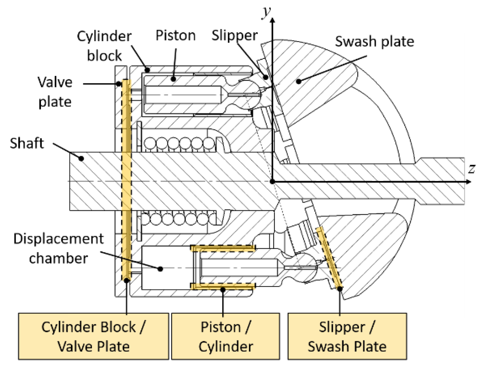
Figure 1.
Cross-section of swash plate type axial piston machine with lubricating interfaces.
Figure 1.
Cross-section of swash plate type axial piston machine with lubricating interfaces.
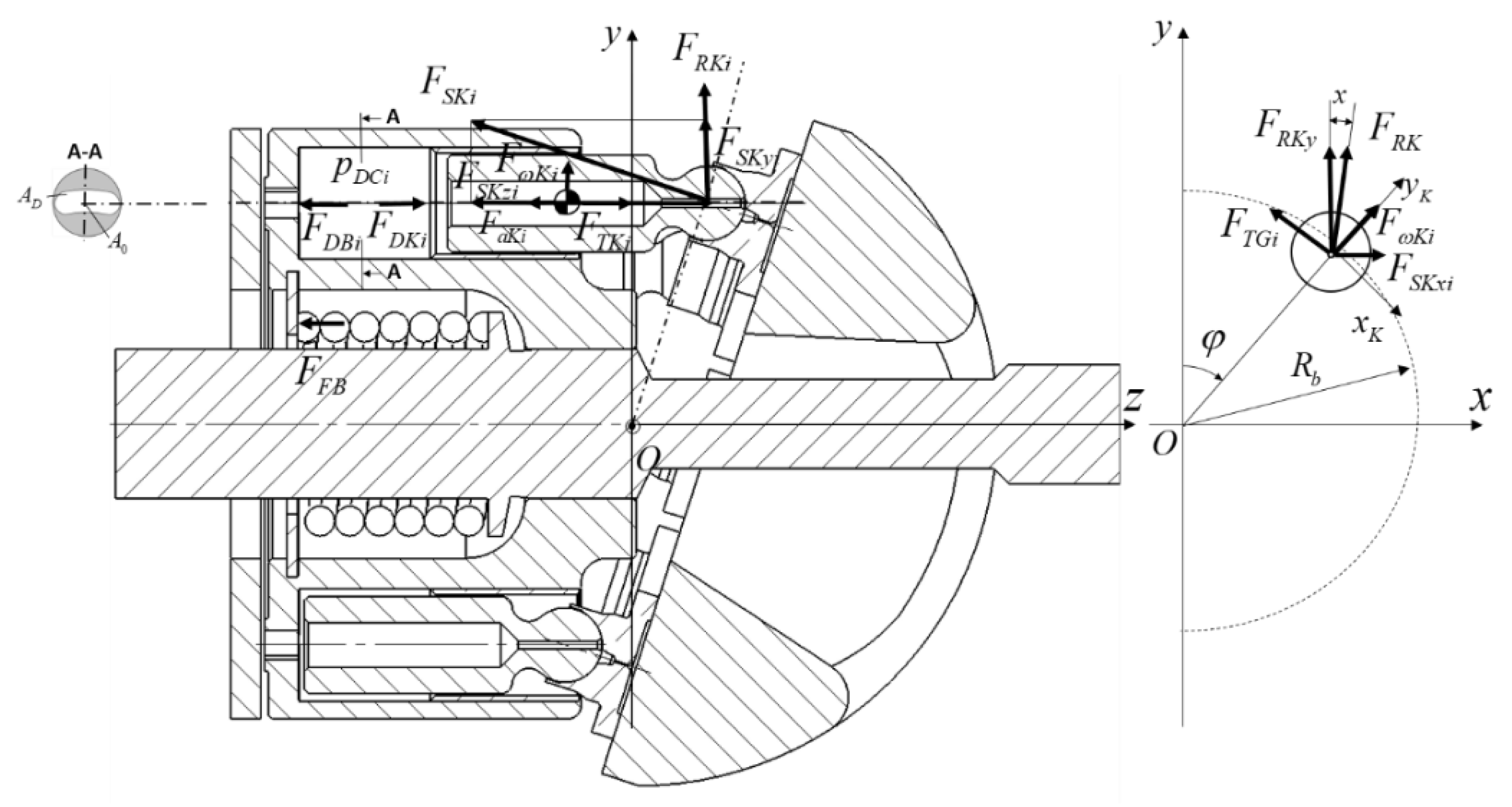
Figure 2.
Free body diagram of the forces acting on the piston/slipper assembly.
Figure 2.
Free body diagram of the forces acting on the piston/slipper assembly.
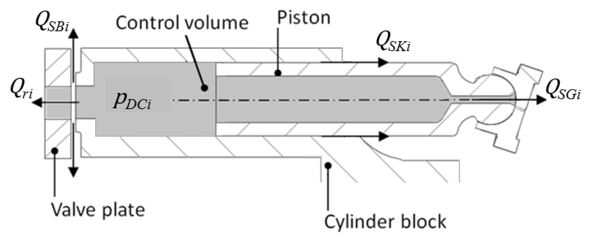
Figure 3.
Instantaneous pressure calculation control volume.
Figure 3.
Instantaneous pressure calculation control volume.
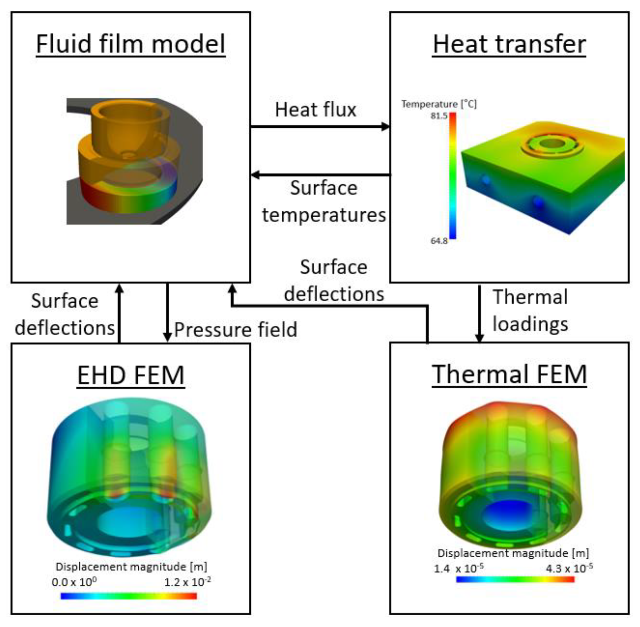
Figure 4.
Lubricating interfaces thermo-elastohydrodynamic model structure.
Figure 4.
Lubricating interfaces thermo-elastohydrodynamic model structure.
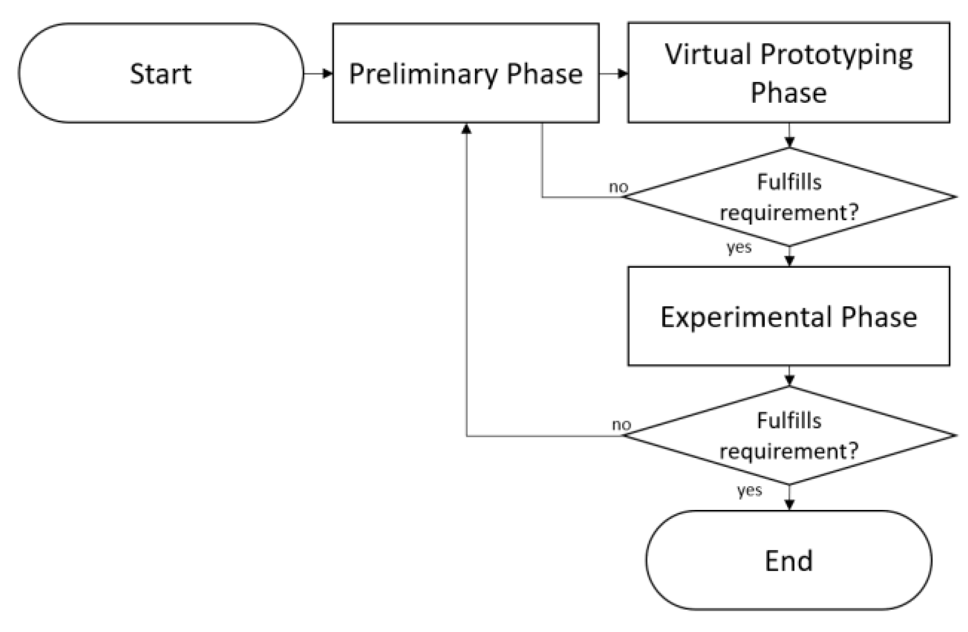
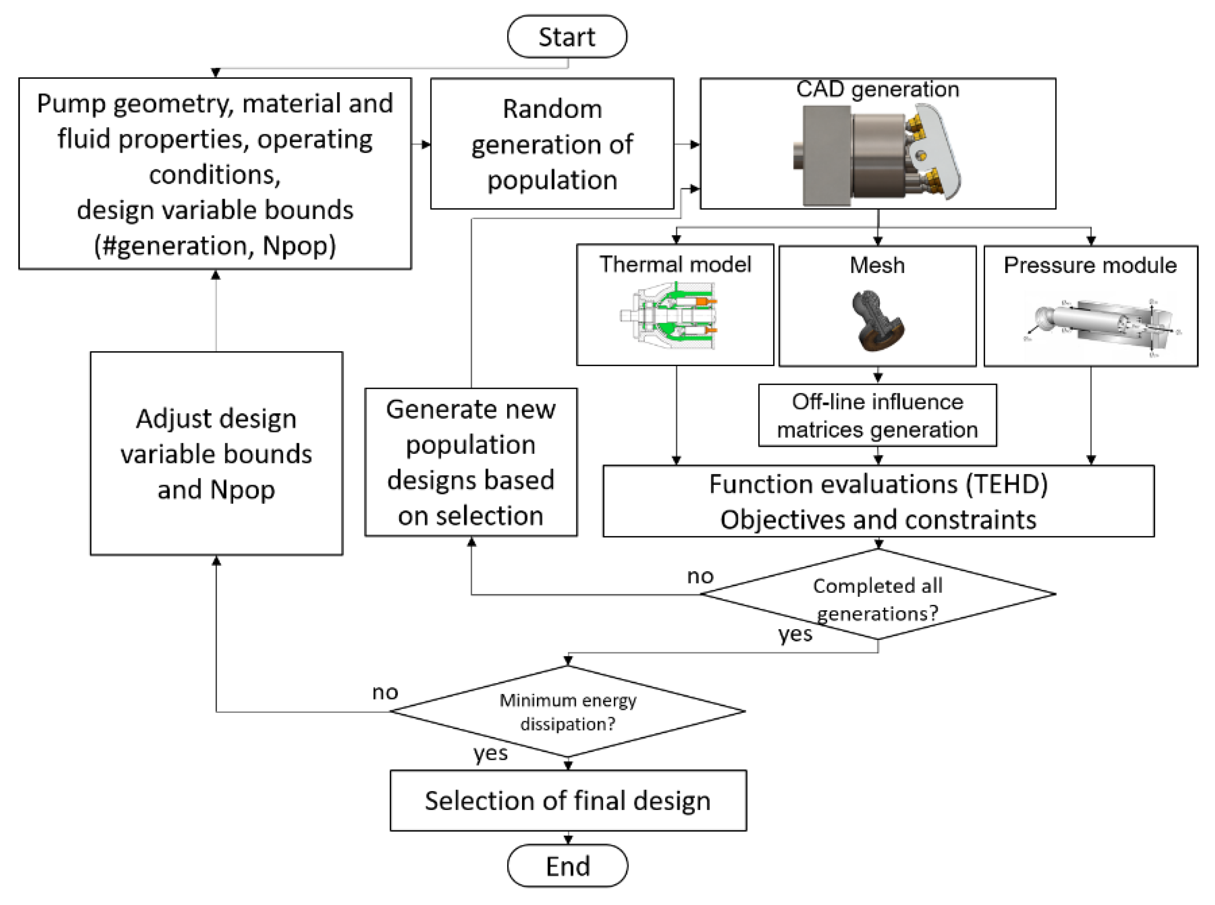
Figure 5.
Virtual prototyping flowchart.
Figure 5.
Virtual prototyping flowchart.
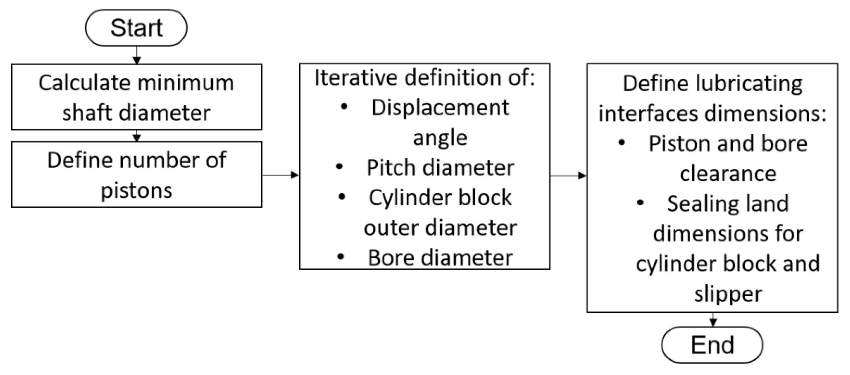
Figure 6.
Preliminary phase flow diagram.
Figure 6.
Preliminary phase flow diagram.
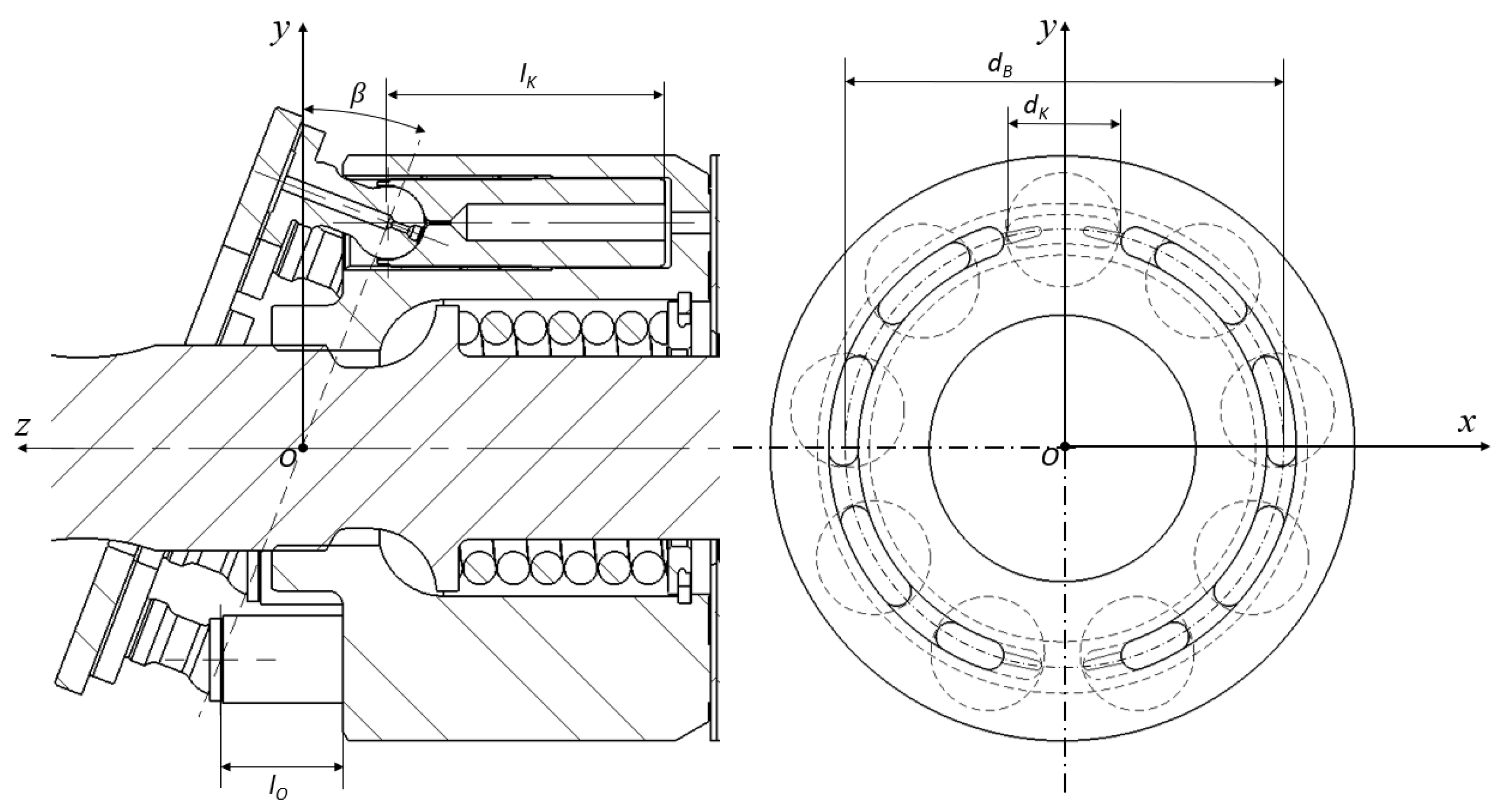
Figure 7.
Main geometrical dimension of axial piston machines of swash plate type.
Figure 7.
Main geometrical dimension of axial piston machines of swash plate type.
Figure 8.
Virtual prototyping flowchart.
Figure 8.
Virtual prototyping flowchart.
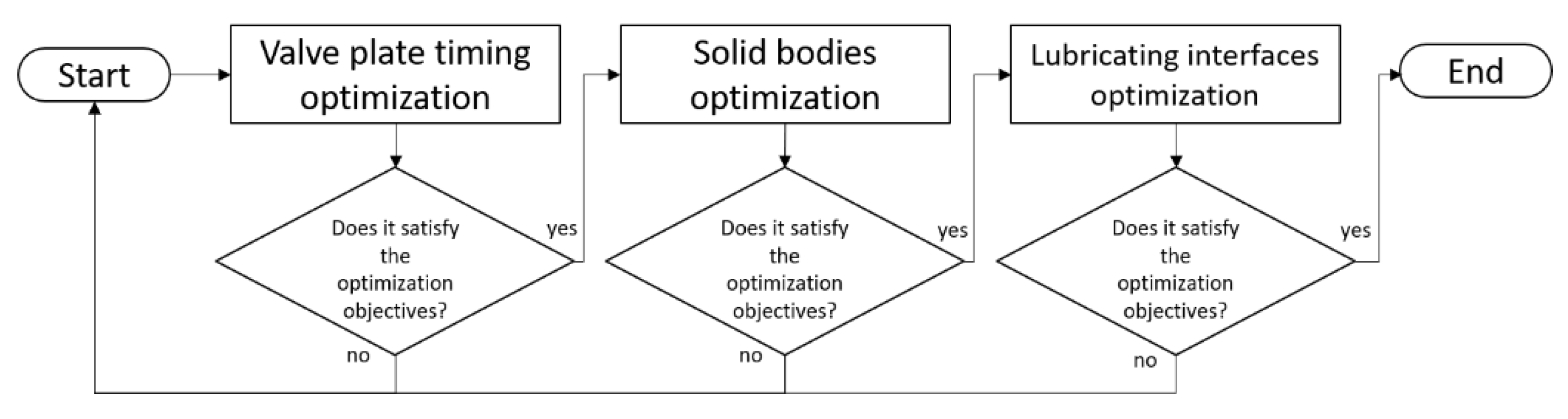
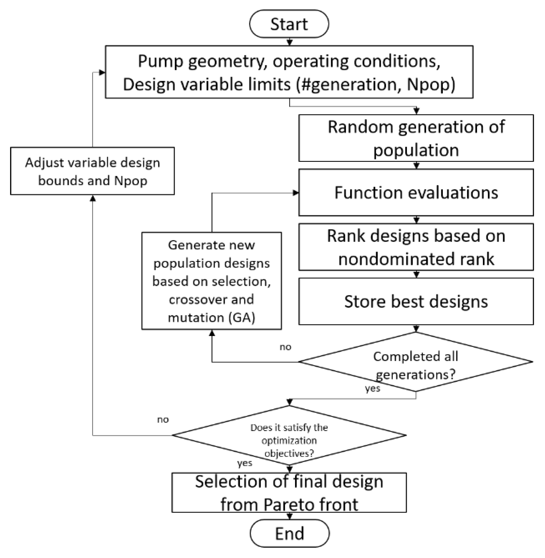
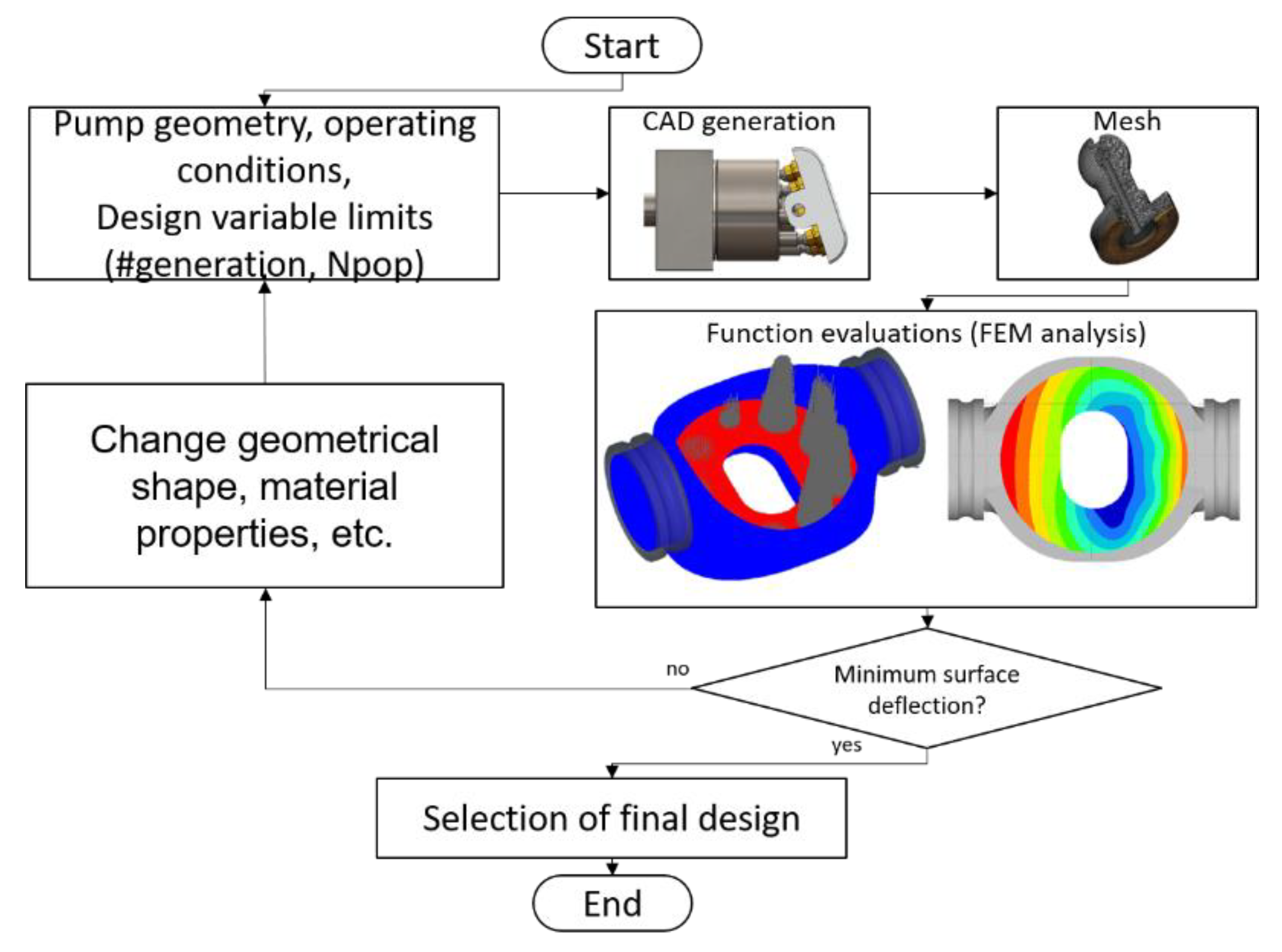
Figure 9.
Valve plate optimization flowchart.
Figure 9.
Valve plate optimization flowchart.
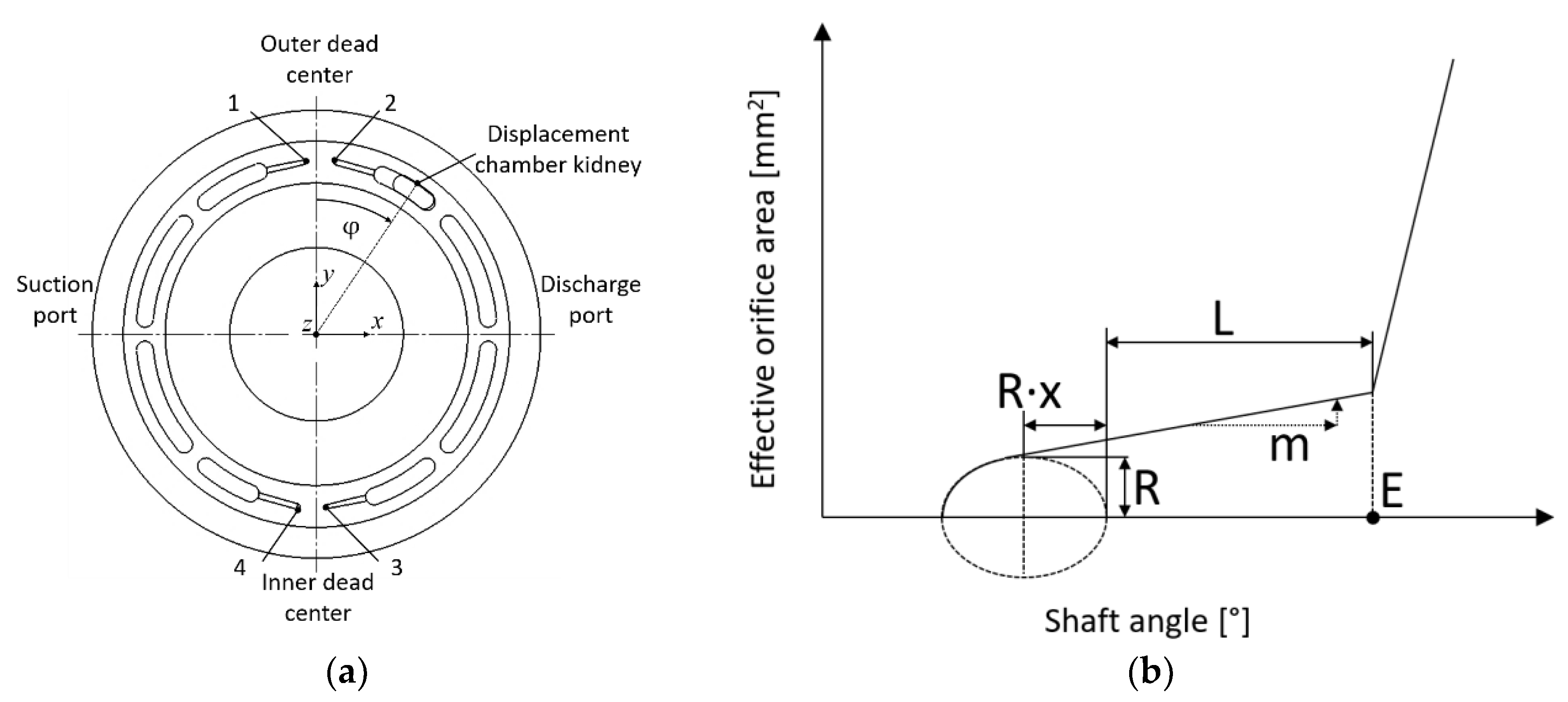
Figure 10.
Valve plate top view (a) and nonlinear groove area opening profile (b).
Figure 10.
Valve plate top view (a) and nonlinear groove area opening profile (b).
Figure 11.
Valve plate optimization results Volumetric Efficiency vs ∆Qhp (a) and Volumetric Efficiency vs ∆Mx (b).
Figure 11.
Valve plate optimization results Volumetric Efficiency vs ∆Qhp (a) and Volumetric Efficiency vs ∆Mx (b).
Figure 12.
Area file as a function of the shaft angle.
Figure 12.
Area file as a function of the shaft angle.
Figure 13.
Example of a swash plate pressure field calculated in the TEHD model.
Figure 13.
Example of a swash plate pressure field calculated in the TEHD model.
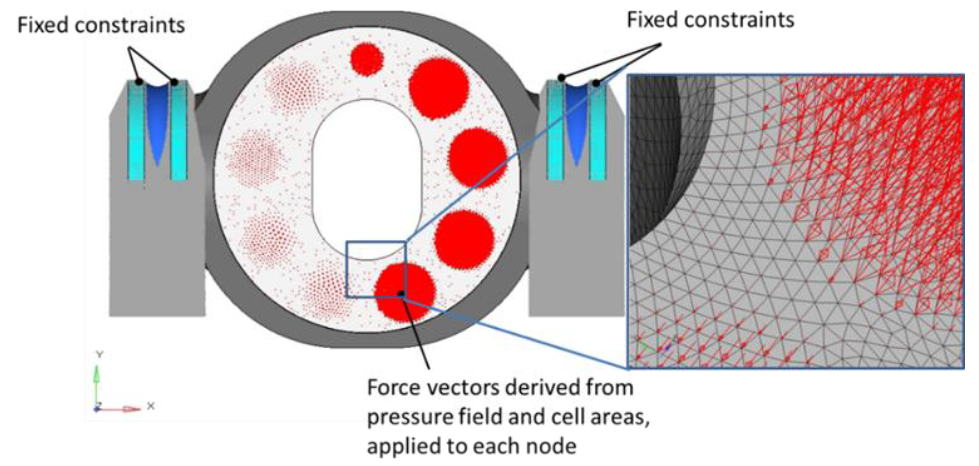
Figure 14.
Example of the swash plate pressure boundaries applied to the three-dimensional mesh.
Figure 14.
Example of the swash plate pressure boundaries applied to the three-dimensional mesh.
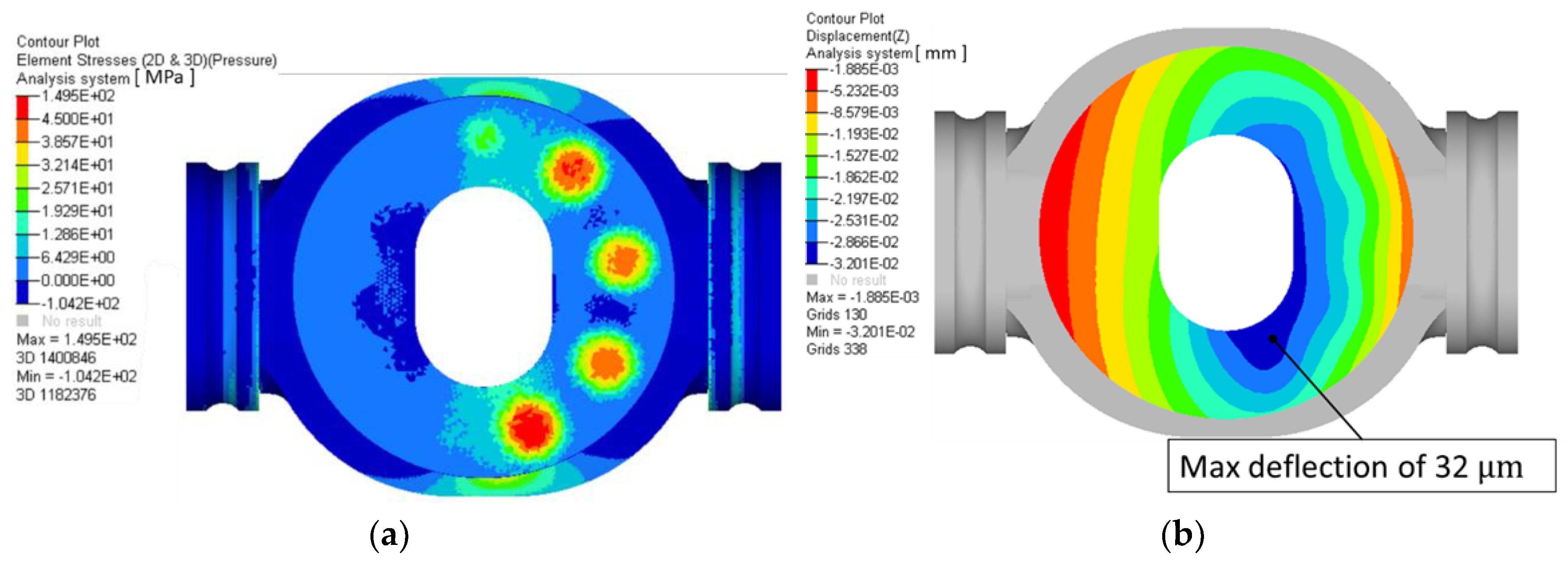
Figure 15.
Example of swash plate von Mises stress distribution on loaded swash plate (a) and surface deformation of the sliding surface in the normal direction to the surface (b).
Figure 15.
Example of swash plate von Mises stress distribution on loaded swash plate (a) and surface deformation of the sliding surface in the normal direction to the surface (b).
Figure 16.
Lubricating interfaces general design methodology.
Figure 16.
Lubricating interfaces general design methodology.
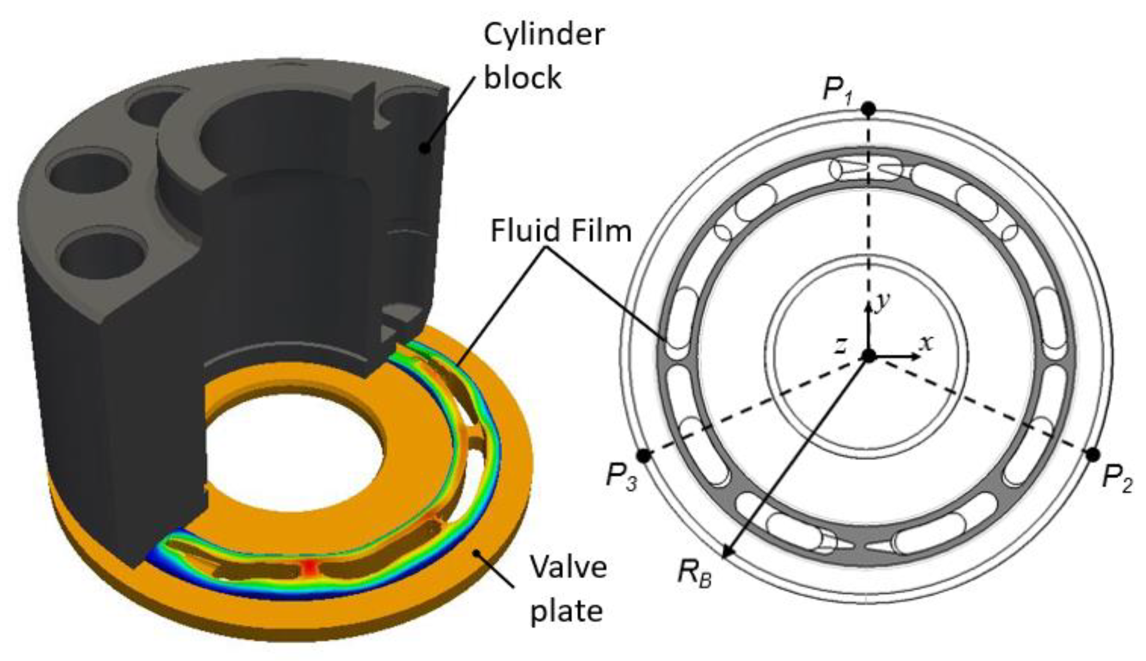
Figure 17.
Cylinder block/valve plate interface representation.
Figure 17.
Cylinder block/valve plate interface representation.
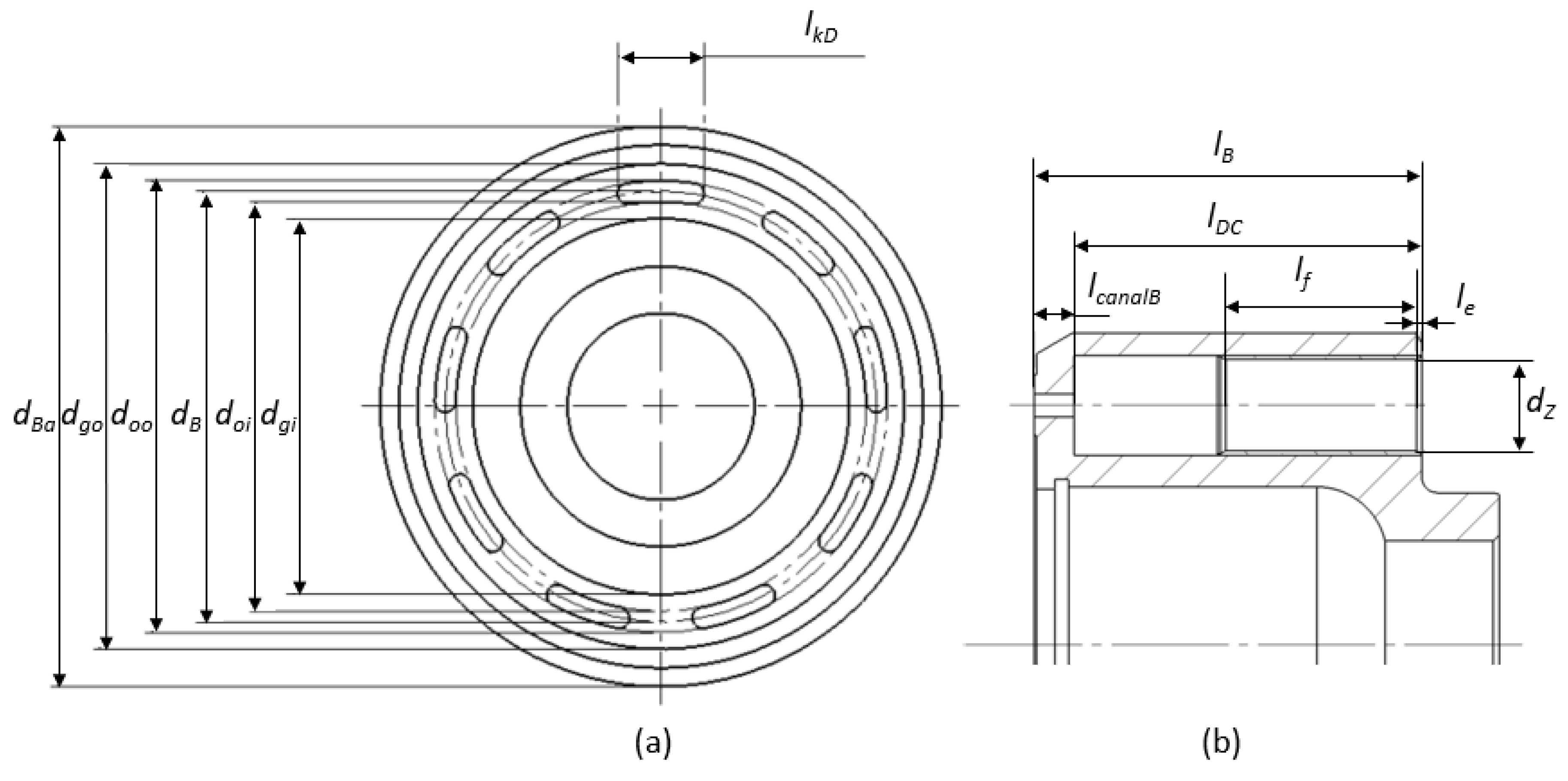
Figure 18.
Main dimensions impacting the cylinder block/valve plate interface. Cylinder block’s bottom view with sealing land dimensions (a) and lateral cross section with main dimensions (b).
Figure 18.
Main dimensions impacting the cylinder block/valve plate interface. Cylinder block’s bottom view with sealing land dimensions (a) and lateral cross section with main dimensions (b).
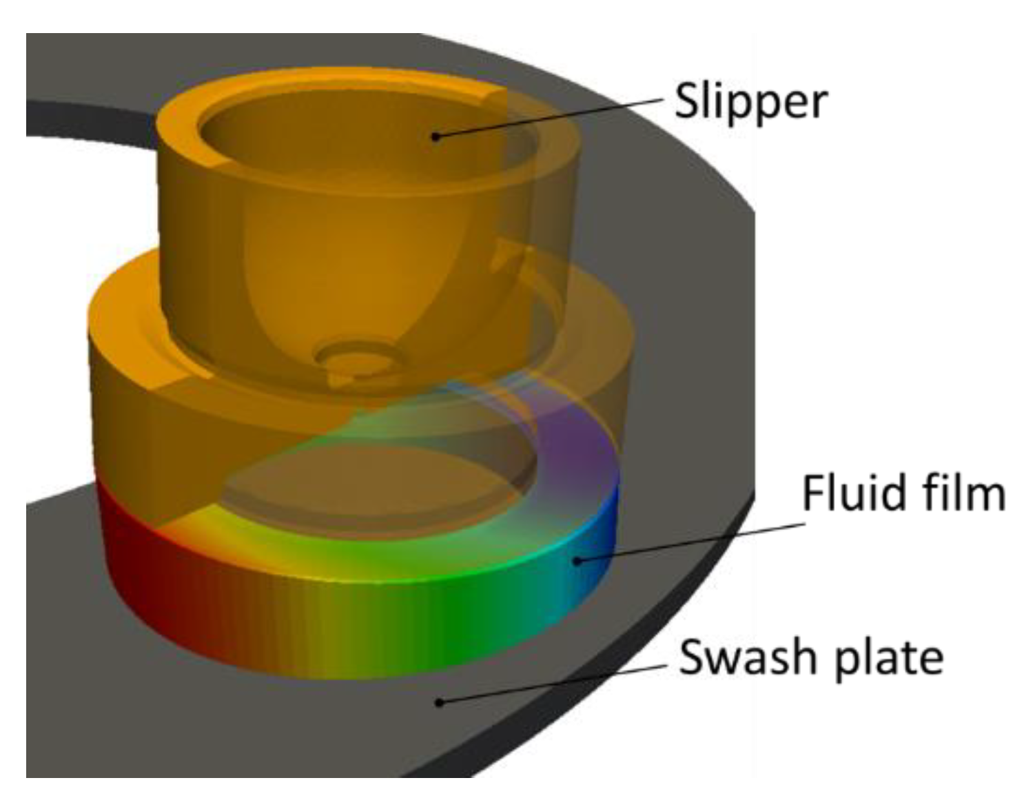
Figure 19.
Slipper/swash plate interface schematic.
Figure 19.
Slipper/swash plate interface schematic.
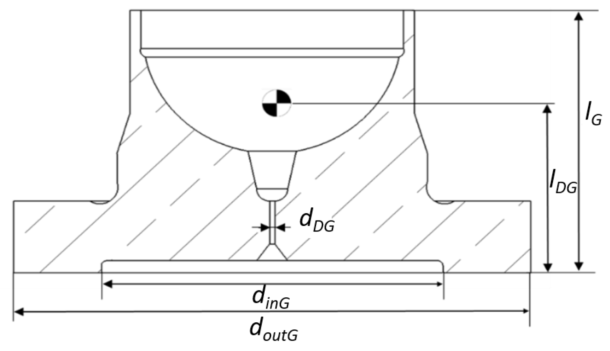
Figure 20.
Slipper main dimensions.
Figure 20.
Slipper main dimensions.
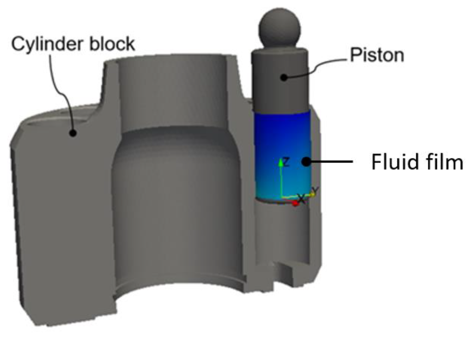
Figure 21.
Piston/cylinder interface schematic.
Figure 21.
Piston/cylinder interface schematic.
Figure 22.
Main dimensions impacting the piston/cylinder interface.
Figure 22.
Main dimensions impacting the piston/cylinder interface.
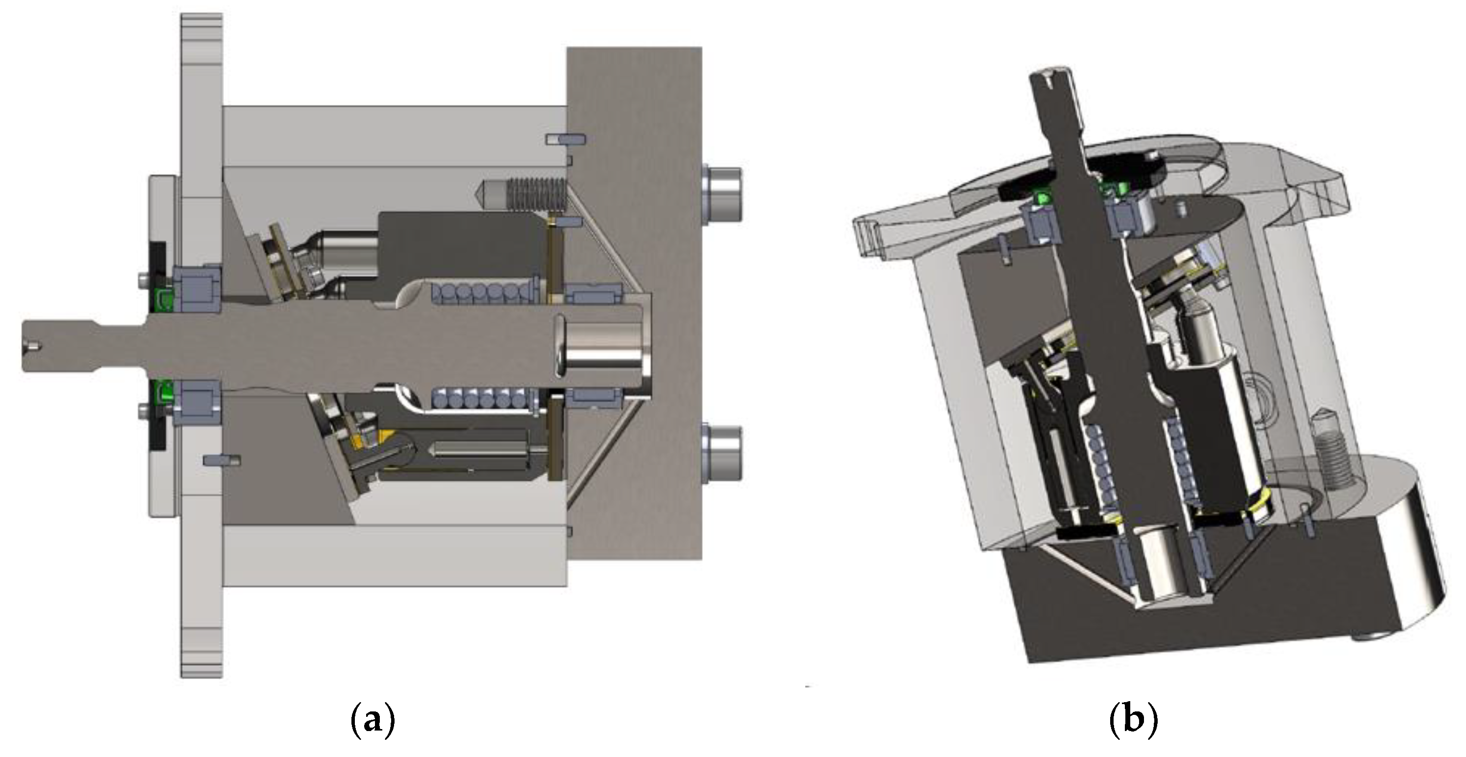
Figure 23.
Closed circuit prototype computational model. Cross-section lateral view (a) and isometric view (b) are shown.
Figure 23.
Closed circuit prototype computational model. Cross-section lateral view (a) and isometric view (b) are shown.
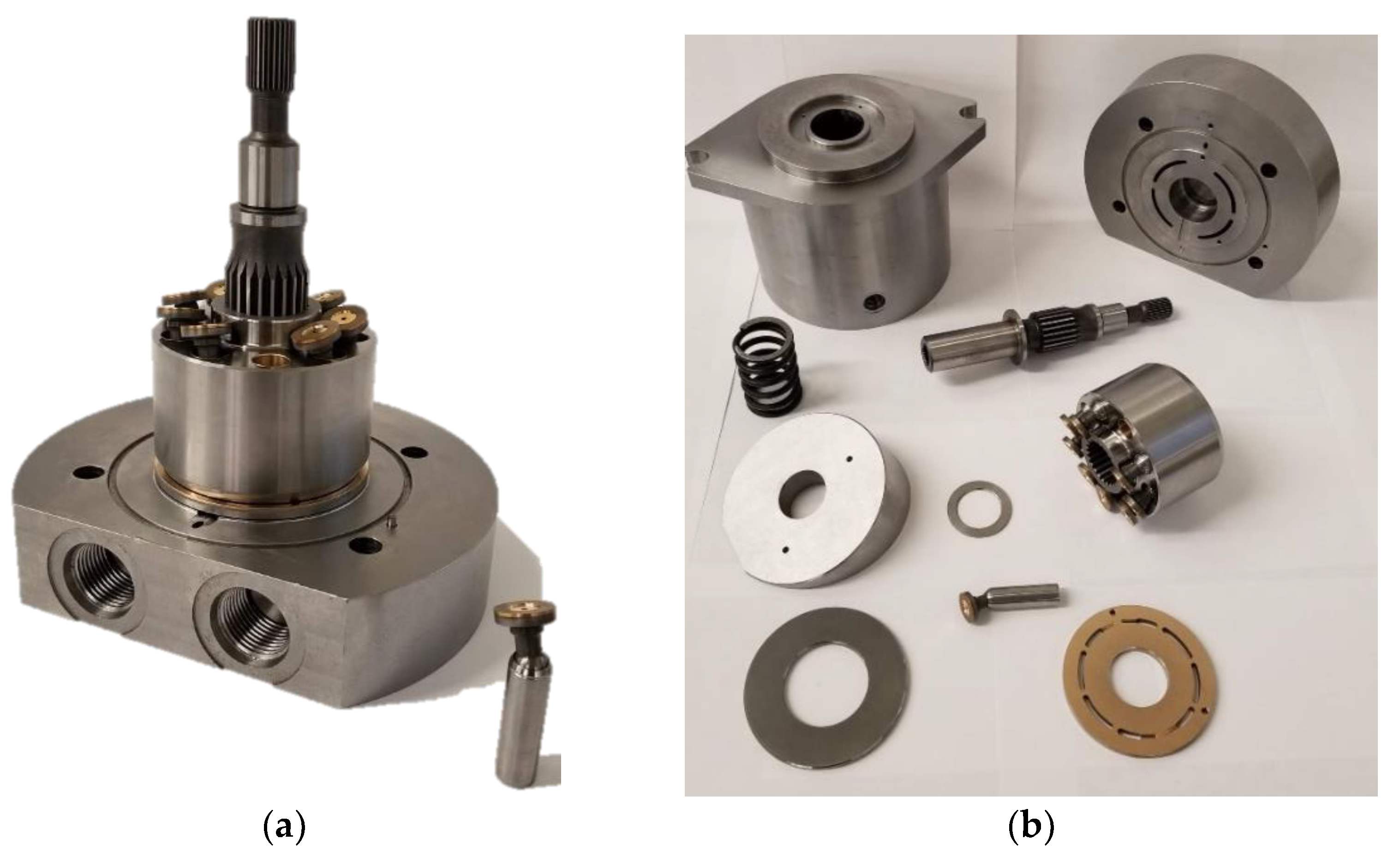
Figure 24.
Closed circuit physical prototype.
Figure 24.
Closed circuit physical prototype.
Figure 25.
Steady state test rig with 24 cc prototype mounted.
Figure 25.
Steady state test rig with 24 cc prototype mounted.
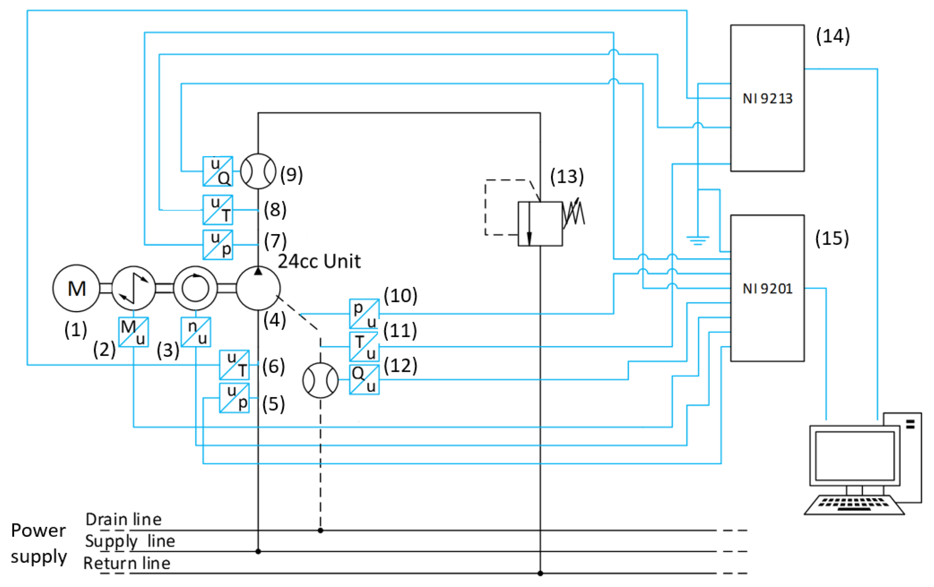
Figure 26.
ISO schematic of the steady-state test rig.
Figure 26.
ISO schematic of the steady-state test rig.
Figure 27.
Prototype efficiencies at n = 1000 rpm, T = 52 °C, and Δp = 50–400 bar.
Figure 27.
Prototype efficiencies at n = 1000 rpm, T = 52 °C, and Δp = 50–400 bar.
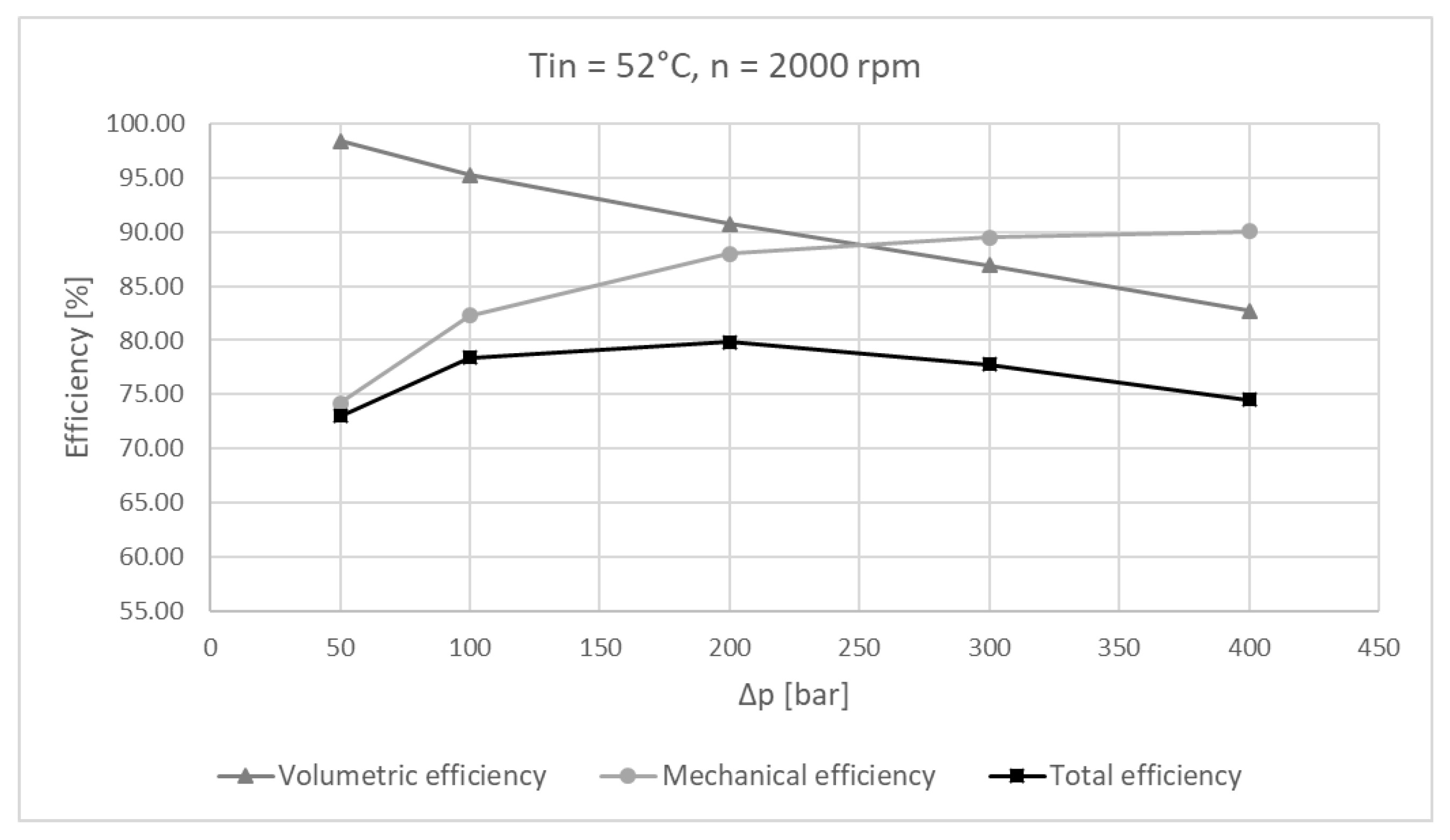
Figure 28.
Prototype efficiencies at n = 2000 rpm, T = 52 °C, and Δp = 50–400 bar.
Figure 28.
Prototype efficiencies at n = 2000 rpm, T = 52 °C, and Δp = 50–400 bar.
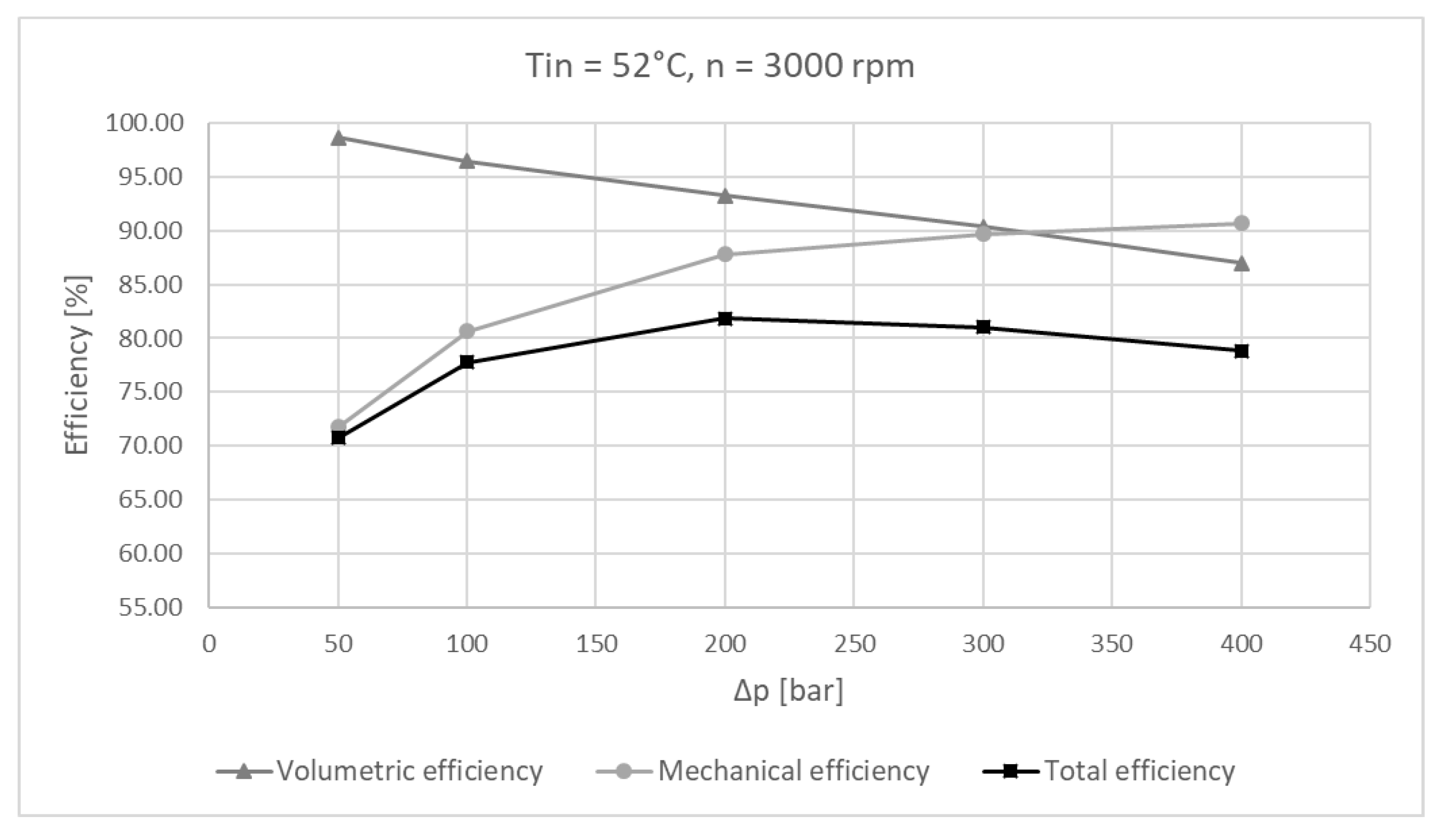
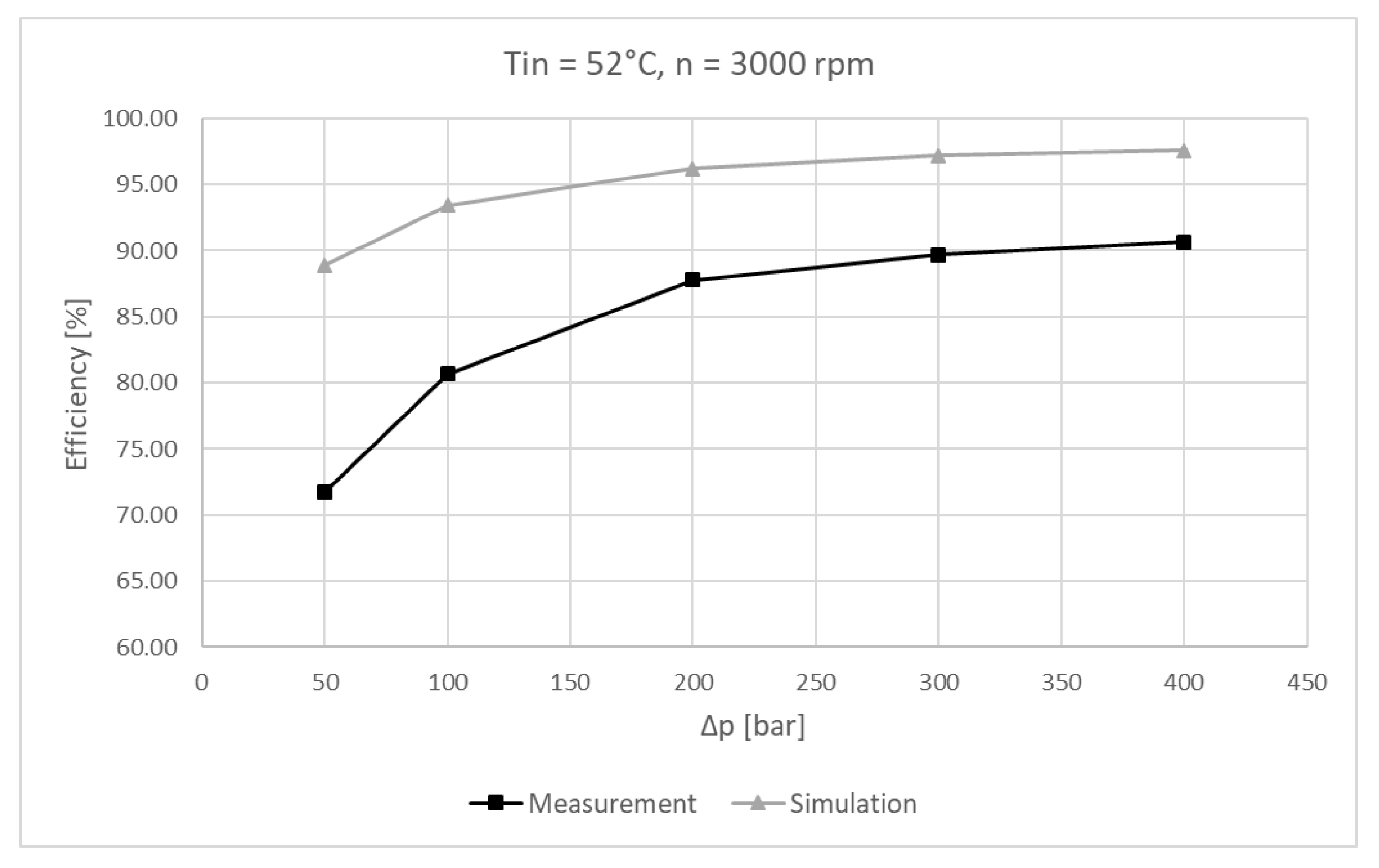
Figure 29.
Prototype efficiencies at n = 3000 rpm, T = 52 °C, and Δp = 50–400 bar.
Figure 29.
Prototype efficiencies at n = 3000 rpm, T = 52 °C, and Δp = 50–400 bar.
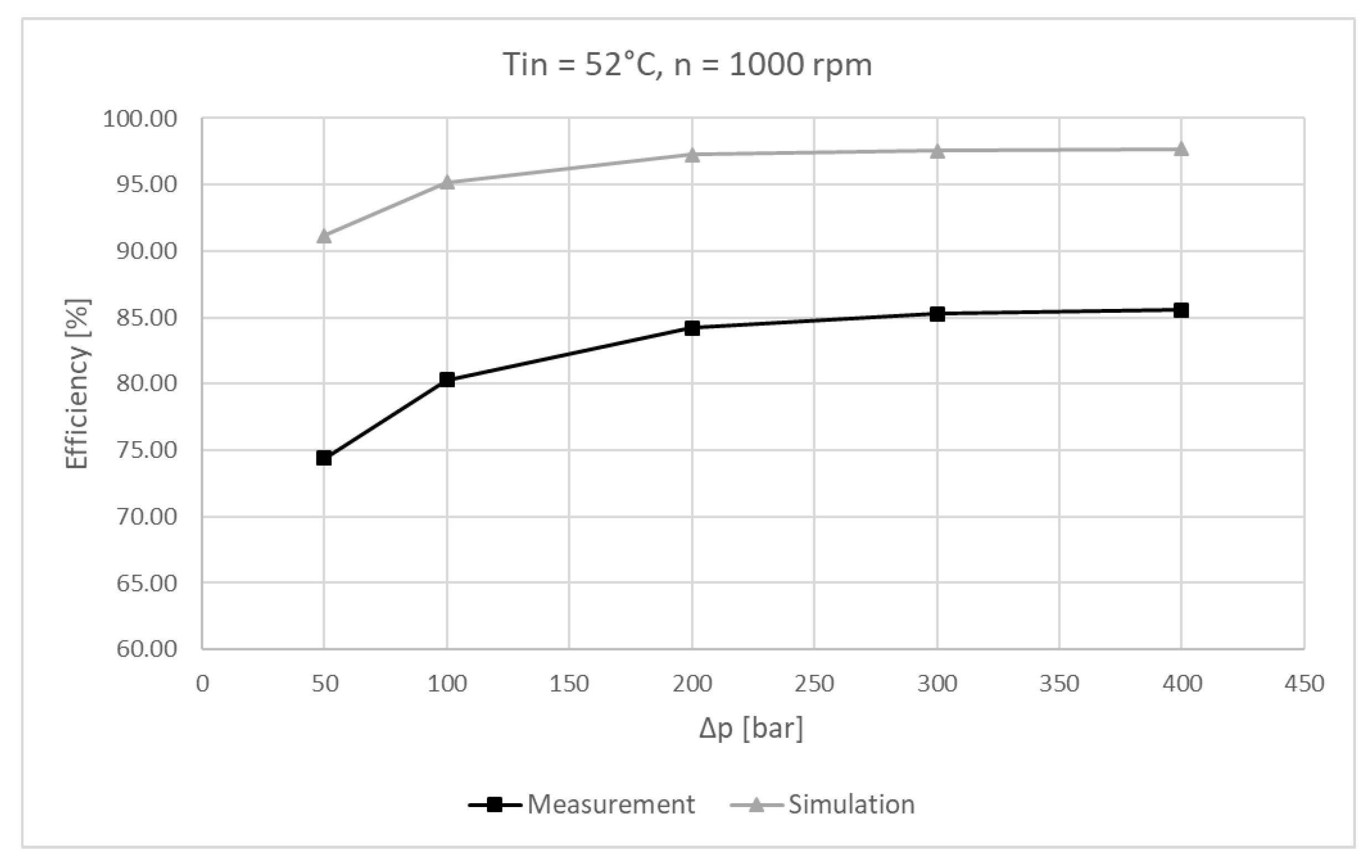
Figure 30.
Volumetric efficiency measured compared against simulated at n = 1000 rpm, T = 52 °C, and Δp = 50–400 bar.
Figure 30.
Volumetric efficiency measured compared against simulated at n = 1000 rpm, T = 52 °C, and Δp = 50–400 bar.
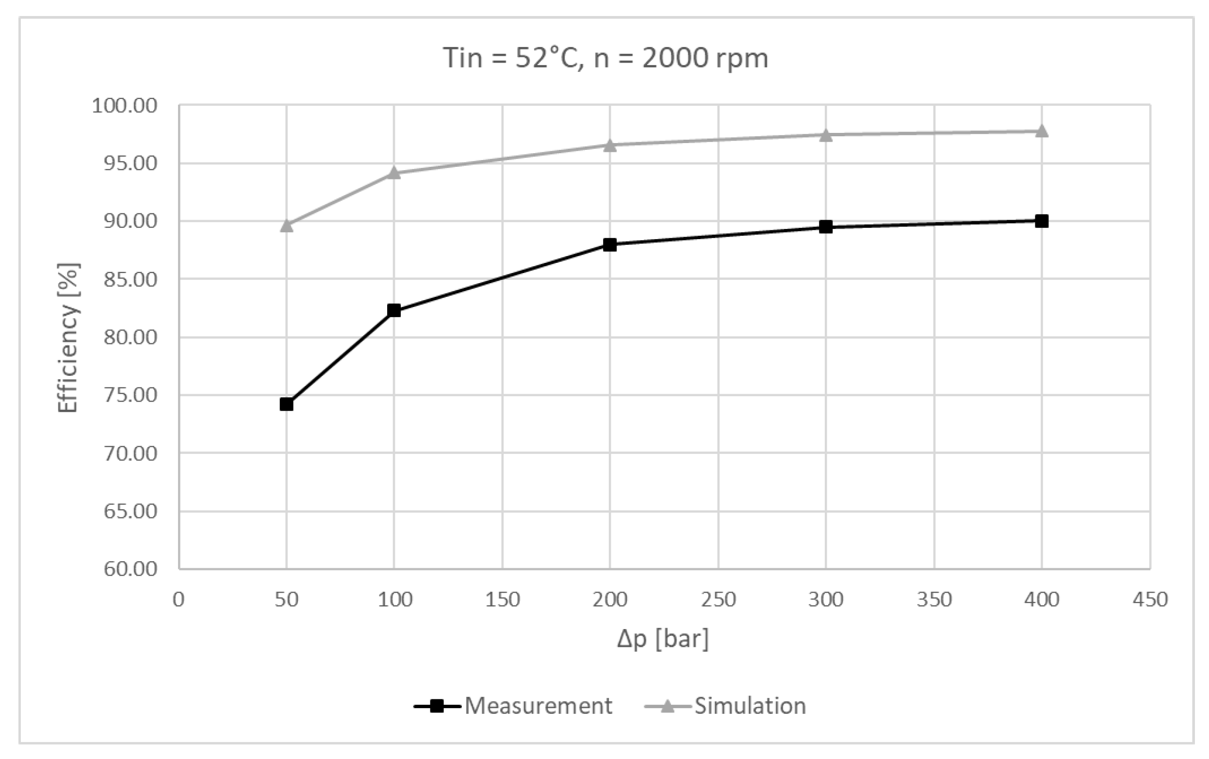
Figure 31.
Volumetric efficiency measured compared against simulated at n = 2000 rpm, T = 52 °C, and Δp = 50–400 bar.
Figure 31.
Volumetric efficiency measured compared against simulated at n = 2000 rpm, T = 52 °C, and Δp = 50–400 bar.
Figure 32.
Volumetric efficiency measured compared against simulated at n = 3000 rpm, T = 52 °C, and Δp = 50–400 bar.
Figure 32.
Volumetric efficiency measured compared against simulated at n = 3000 rpm, T = 52 °C, and Δp = 50–400 bar.
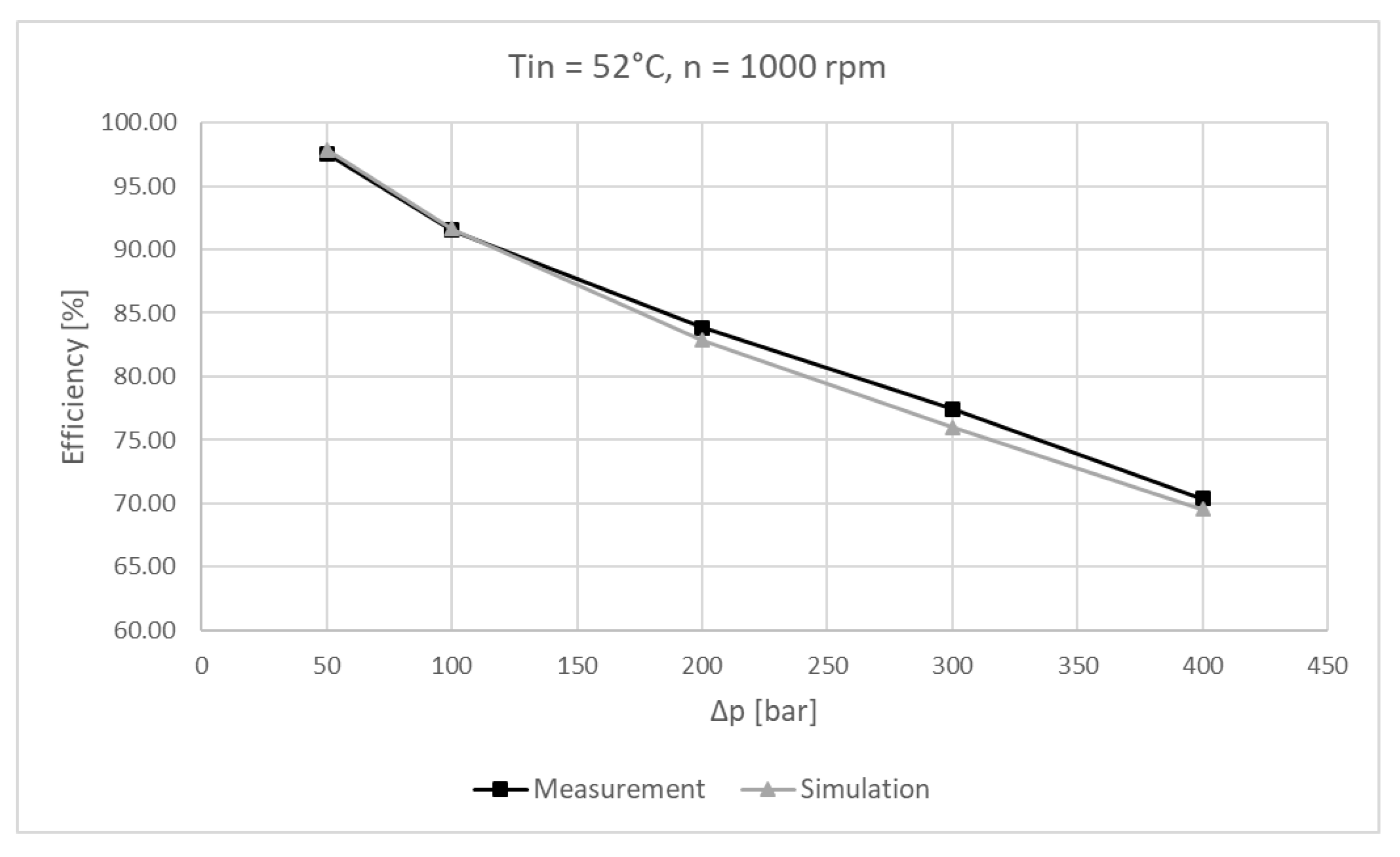
Figure 33.
Mechanical efficiency measured compared against simulated at n = 1000 rpm, T = 52 °C, and Δp = 50–400 bar.
Figure 33.
Mechanical efficiency measured compared against simulated at n = 1000 rpm, T = 52 °C, and Δp = 50–400 bar.
Figure 34.
Mechanical efficiency measured compared against simulated at n = 2000 rpm, T = 52 °C, and Δp = 50–400 bar.
Figure 34.
Mechanical efficiency measured compared against simulated at n = 2000 rpm, T = 52 °C, and Δp = 50–400 bar.
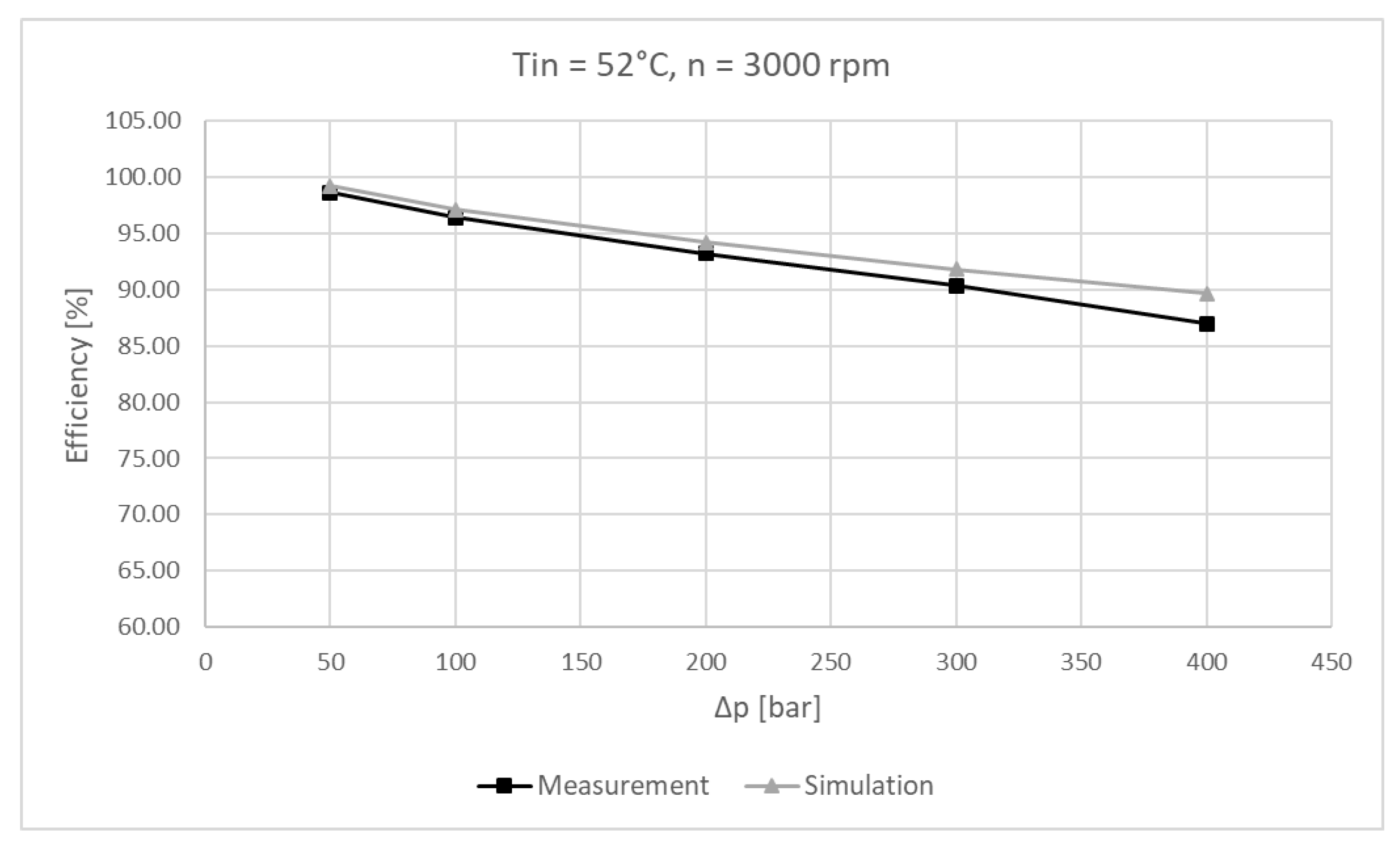
Figure 35.
Mechanical efficiency measured compared against simulated at n = 3000 rpm, T = 52 °C, and Δp = 50–400 bar.
Figure 35.
Mechanical efficiency measured compared against simulated at n = 3000 rpm, T = 52 °C, and Δp = 50–400 bar.
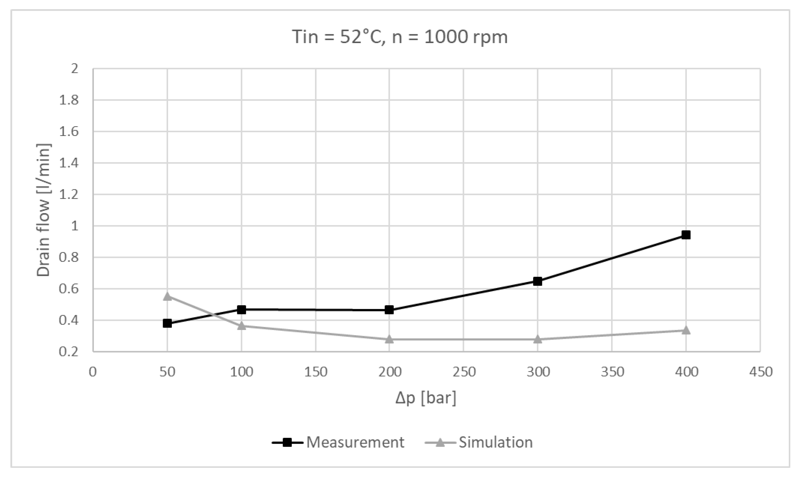
Figure 36.
Drain flow measured compared against simulated at n = 1000 rpm, T = 52 °C, and Δp = 50–400 bar.
Figure 36.
Drain flow measured compared against simulated at n = 1000 rpm, T = 52 °C, and Δp = 50–400 bar.
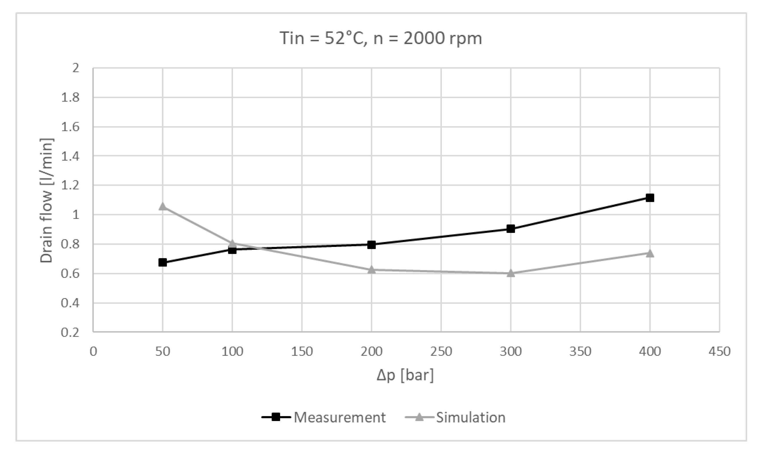
Figure 37.
Drain flow measured compared against simulated at n = 2000 rpm, T = 52 °C, and Δp = 50–400 bar.
Figure 37.
Drain flow measured compared against simulated at n = 2000 rpm, T = 52 °C, and Δp = 50–400 bar.
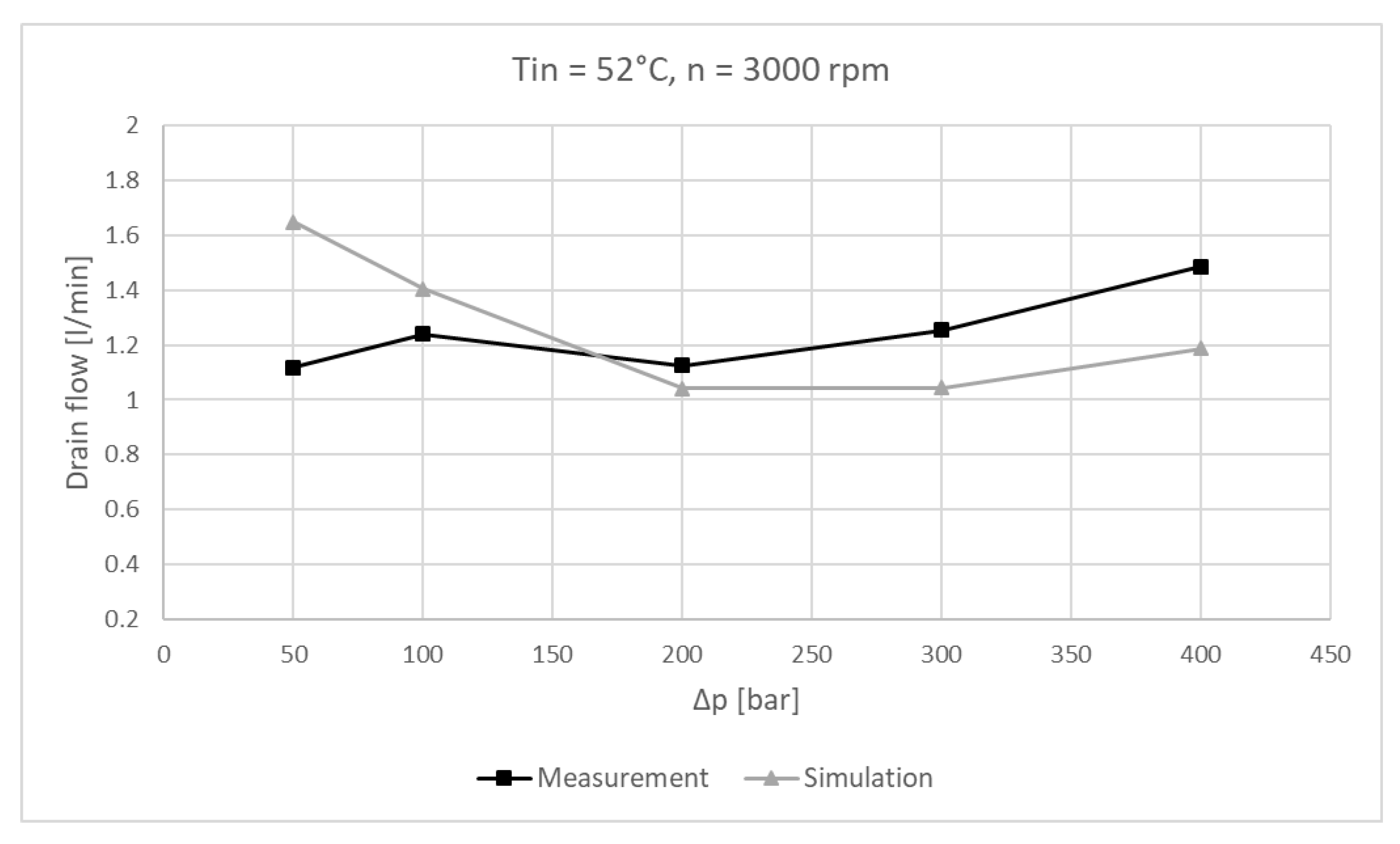
Figure 38.
Drain flow measured compared against simulated at n = 3000 rpm, T = 52 °C, and Δp = 50–400 bar.
Figure 38.
Drain flow measured compared against simulated at n = 3000 rpm, T = 52 °C, and Δp = 50–400 bar.
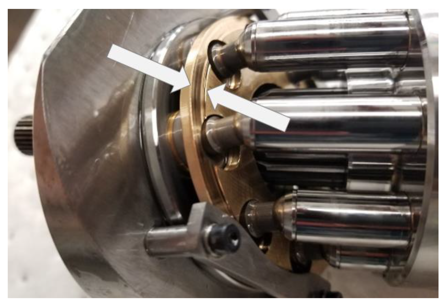
Figure 39.
Worn slipper retainer plate after measurements.
Figure 39.
Worn slipper retainer plate after measurements.
Table 1.
Cost functions for the valve plate optimization.
Table 1.
Cost functions for the valve plate optimization.
| Cost Functions |
|---|
| f1() = Leakage (%) |
| f2() = ∆Qhp (L/min) |
| f3() = ∆Mx (Nm) |
| f4() = ∆My (Nm) |
| f5() = (Nm) |
Table 2.
Material properties influencing the lubricating interfaces’ behavior.
Table 2.
Material properties influencing the lubricating interfaces’ behavior.
| Description | Symbol | Unit |
|---|
| Young’s modulus | E | (Pa) |
| Poisson’s ratio | ν | (-) |
| Density | ρ | (kg/m3) |
| Thermal conductivity | λ | (W/mK) |
| Coefficient of linear thermal expansion | α | (-) |
Table 3.
Operating conditions.
Table 3.
Operating conditions.
| Operating Condition | Speed (rpm) | Δp (bar) | Displacement (%) |
|---|
| 1 | max | max | max |
| 2 | max | max | min |
| 3 | max | min | min |
| 4 | max | min | max |
| 5 | min | max | max |
| 6 | min | max | min |
| 7 | min | min | min |
| 8 | min | min | max |
| 9 | min | max | moderate |
| 10 | moderate | max | max |
Table 4.
Operating conditions range.
Table 4.
Operating conditions range.
| Description | Specification |
|---|
| Pressure differential | 50, 100, 200, 300, 400 (bar) |
| Speed | 1000, 2000, 3000 (rpm) |
| Displacement | 100 (%) |
| Temperature | 42, 52, 72 (°C) |
Table 5.
Test rig set up components.
Table 5.
Test rig set up components.
| ID | Description | Specification |
|---|
| 1 | Electric drive | Max power: 225 Kw, Max torque 615 Nm @3500 rpm |
| 2, 3 | Staiger Mohilo torque cell | 0–500 Nm range, error ±0.2% of full scale |
| 4 | Closed circuit pump | 24cc, fixed displacement, max torque 160 Nm @Δp = 400 bar |
| 5 | Pressure transducer | WIKA S-10, 0–100 bar, 0.125% BFSL |
| 6, 8, 11 | Thermocouple | Omega K-type Thermocouple, 2.2 °C error limit |
| 7 | Pressure transducer | HYDAC HAD 4445, 0.5% BFSL |
| 9 | Flowmeter | VSE VS 10 Gear type, 1.2–250 L/min, 0.3% accuracy |
| 10 | Pressure transducer | WIKA S-10, 0–25 bar, 0.125% BFSL |
| 12 | Flowmeter | VSE VS 0.2 Gear type, 0.02–18 L/min, 0.3% accuracy |
| 13 | Pressure relief | Max flow 350 L/min |
| 14 | DAQ | NI cDAQ, NI 9213 |
| 15 | DAQ | NI cDAQ, NI 9201 |


