Article

Effect of Airtightness on Thermal Loads in Legacy Low-Income Housing

by
Samuel Domínguez-Amarillo
,
Jesica Fernández-Agüera
*,
Miguel Ángel Campano
and
Ignacio Acosta
Instituto Universitario de Arquitectura y Ciencias de la Construcción, Escuela Técnica Superior de Arquitectura, Universidad de Sevilla, 41014 Sevilla, Spain
*
Author to whom correspondence should be addressed.
Energies 2019, 12(9), 1677; https://doi.org/10.3390/en12091677
Submission received: 3 March 2019 / Revised: 20 April 2019 / Accepted: 29 April 2019 / Published: 2 May 2019
(This article belongs to the Section G: Energy and Buildings)

Abstract

:
Spain’s high winter weather-associated death count, the second largest in Europe, can be attributed primarily to the low construction standards of its social housing, particularly the stock built prior to the entry into effect of the earliest statutory provisions on envelope quality. Hence, improving building envelopes to both reduce energy consumption and raise occupant comfort levels is important. Air leakage is one of the factors with the greatest impact on indoor comfort and domestic energy consumption. This study explores the sensitivity of energy consumption to that parameter in a series of types of social housing built between 1950 and 1979 in five Mediterranean climate zones. Demand in a total of 53 housing units located in 21 developments was simulated to that end. The findings show that air permeability has a significant effect on wintertime demand in the sample studied. Although the impact is greater in the more severe climates where it is estimated to be over 10 kWh/m2, it may also affect energy consumption in mild climates.

1. Introduction

Spain is the European country with the second-highest number of winter-related deaths [1]. That statistic is due primarily to poor construction standards, especially in low-income housing with no environmental control systems. Envelope airtightness or uncontrolled indoor–outdoor air exchange is one of the key variables in residential energy consumption and comfort.
The method most commonly accepted by the scientific community to assess airtightness is the blower door test. A number of studies have been conducted on airtightness in single-family homes in northern Europe [2,3,4,5,6] and the United States [7,8,9] over the last three decades. It has also been an emerging field of research over the last 10 years in southern Europe, Spain included [10,11,12,13,14], where the Infiles research project [15] presently underway has been enlarging the country’s airtightness database [16,17,18,19,20] using a standardised measuring protocol to ensure comparability of the findings.
Most of the literature quantifying the energy demand associated with infiltration reports on conditions in northern Europe, where the energy impact of air infiltration on heating demand is estimated to be in the order of 10 kWh/m2 in moderately cold regions (2500 degree-days at 20 °C) [21]. This question has been scantly studied in Spain, however, although some research has been conducted in mild [22] and continental-like climates. In one study, the energy impact of infiltrations was assessed using a simplified model (Equation (1)) based on the degree-day concept that relates the mean outdoor to the indoor comfort temperature (21 °C for heating and 25 °C for cooling). While actual energy consumption depends on the specific temperature prevailing in any given dwelling, this theoretical model can be used to determine the impact of air inflow, specific air capacity, and the indoor–outdoor temperature difference on energy demand in the locations where the tests are performed [18]. Meiss and Feijó [23], analysing 13 housing units in northern Spain, were the first to address the subject from an energy perspective. They estimated the impact of infiltration on energy demand in housing built on the existing technical building code [24] to range from 10.5% to 27.4%; in units constructed under the former code [25], from 21.9% and 27%; and in those dating prior to 1979 but retrofitted by their occupants, from 11.3% to 13%:
Qinf = Cp · Gt · Vinf
where
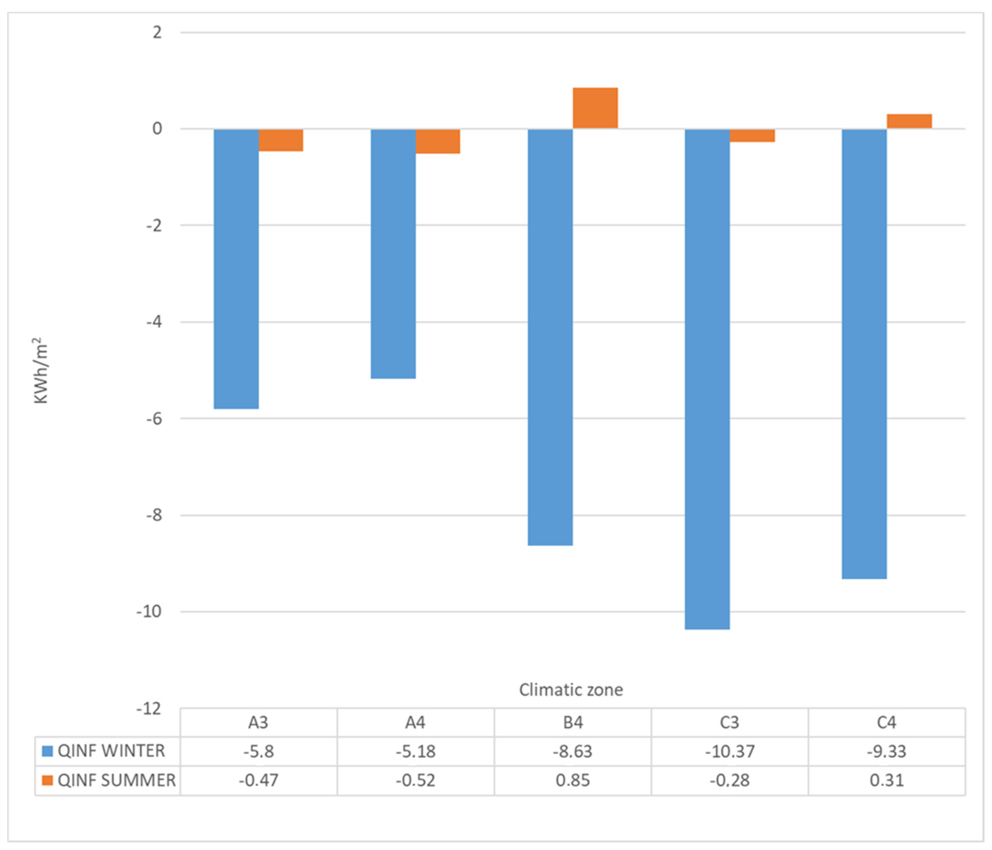
  • Qinf is the annual air infiltration-induced energy loss (kWh/year) for heating QinfH and cooling QinfC, expressed per unit area;
  • Cp is the specific heat capacity of air, assumed to be 0.34 Wh/m3·K;
  • Gt is the annual degree-days (kKh/year), assuming a baseline comfort temperature of 21 °C for heating (GtH) and of 25 °C for cooling (GtC); and
  • Vinf is the air leakage rate (m3/h).
The conclusion reached was that losses attributable to air change are relatively greater in multifamily than in single-family detached housing and are becoming more important in better insulated buildings [26].
This study aims primarily to analyse the vulnerability to air leakage of the envelopes of social housing built prior to entry in effect CT79, Spain’s first legislation on the subject [24]. This aspect is very important for the cost-optimal analysis applications in Europe since the Energy Performance of Buildings Directive (EPBD) recast [27].

2. Materials and Methods

2.1. Characterisation of Social Housing and Sampling

A study of social housing typologies and characteristics in southern Spain [28,29,30] laid the ground for stratified random sampling and the definition of a sample on which to conduct building envelope airtightness tests and energy demand simulation. The attribute defined for stratification was the one deemed to have the greatest potential to induce differences [17,31] in the construction solutions adopted for building envelopes: area-dependent climate [29]. The parameters involved were regarded to possibly play a role in determining envelope performance, once the geometric parameters routinely used and regional construction particularities were identified and further to the characteristics determined for the overall and regional housing stocks. A total of 21 multi-owned housing developments were selected as particularly representative of low-income buildings. The location, year of construction and morphological characteristics of these developments are given in Table 1, a description of their envelopes in Table 2, and their geometry in Figure 1.
The simulations were run using the envelopes found to be specific to each façade model and building type in earlier analysis and classification studies [29,30]. The representative models identified included three types of façade enclosures, two variations on the F1 model and one F2 model, as listed in Table 2. Envelopes were defined on the grounds of their specific mass, constructional composition, energy parameters of the materials and reflectivity and emissivity of the outer façade surface. The variability among enclosures was narrow, for most of the housing built in the period fluctuated between several of those established, as discussed in [29]. The wider range of variation identified in the roofs was factored into the definitions of the building energy models. Briefly, the procedure involved differentiating the buildings on the grounds of their constructional characteristics, morphology and geometry (opening-to-blank wall, wall-to-floor ratios and similar), location and airtightness to mirror actual behaviour as accurately as possible.

2.1.1. Location and Climate

Although the region of southern Spain known as Andalusia has a Mediterranean climate, several sub-zones can be identified, from areas characterised by cold winters (Granada) to others with temperate weather year-round (Almería). More detailed information on the climate zones envisaged in national energy performance legislation is given in [32]. The present study covered the five climate zones most representative of Andalusia, ranging from very mild (zone A) to cold (zone C) winters and warm (zone 3) to hot (zone 4) summers. Separate predictive models were developed for each climate zone. The mean, maximum and minimum temperatures on record for each zone are given in Table 3.

2.1.2. Airtightness

Dwelling envelope airtightness was measured with the standard blower door test implemented as described in [12]. The tests were conducted for an airtightness value of 50 Pa with a Minneapolis Blower Door Model 4 facility featuring ±3% accuracy and an operating range of 25 m3·h−1 to 7800 m3·h−1. Measurements were taken at pressures ranging from 20 Pa to 70 Pa at 5 Pa intervals further to the procedure described in the Spanish and European standard UNE EN 13829:2002 [33]. Airtightness was measured at an infiltration rate of 50 Pa in a total of 53 units located in the 21 developments studied. The mean V50, n50 and q50 values and respective standard deviations listed in Table 4 are discussed in greater detail in [34].
Blower door test values were used to calibrate the models and determine the mean value for subsequent analyses. Vinf was calculated from the test values at a pressure difference of 50 Pa. As the latter do not measure actual dwelling air leakage, however, they had to be converted to equivalent real air flows. Estimating actual infiltration is a complex task, given that wind and temperature conditions throughout the year are difficult to foresee and the test does not deliver precise air leakage data.
The Persily–Kronvall procedure [35], a simple, widely used model, assumes that permeability at 50 Pa is linearly related to mean yearly infiltration (Equation (2)). Sherman [36] developed another simple approach (Equation (3)) from the LBL infiltration model for the annual infiltration rate of detached houses in North America, introducing N, a correlation factor found as the product of factors representing climate zone, wind shielding, house height and crack size. According to extensive measuring undertaken in several European countries as reported by Dubrul in 1988 [26], the denominator in Equation (3) ranges from 10 to 30, depending on building type, wind conditions and leakage distribution.
Here, the value assumed was 20 because the sample consisted of multifamily housing with uniformly distributed leakage, intermediate-sheltered exposure and a mean wintertime meteorological wind speed of under 4 m/s.
n 50 = V 50 20 V .
A C H = n 50 N
where:
  • V is the internal air volume (m3);
  • V50 is the air leakage rate at 50 Pa (m3/h);
  • n50 is the air change rate at 50 Pa (h−1);
  • A C H is air change rate per hour at standard pressure (m3/h);
  • N is a correlation factor.

2.2. Simulation

All simulations were conducted with three levels of airtightness: the airtightness measured for each case plus building leakage rates of n50 = 0.2 h−1 and n50 = 1 h−1. Sensitivity analysis simulations were conducted for 53 flats located in 21 developments, applying their actual exposure to wind conditions (Figure 1). Most of the cases involved sheltered conditions, the type most commonly found in Spain because multifamily dwellings are located primarily in town/city centres where they are surrounded by trees and other buildings. Empirical leakage distribution data were used to calibrate the models.
Building energy assessments were performed for the three airtightness values using Design Builder Essentials software (5.0.2.003) which delivered daily, monthly and yearly demand data for all the case studies using Equation (4) (EN12831 [37]):
A C H = 2 · V · n 50 · τ · ε
where
  • A C H is the air flow at standard pressure (m3/h);
  • n50 is the air change rate at 50 Pa (h−1);
  • V is the indoor air volume (m3);
  • τ is the wind exposure class (coefficient), determined from the façade exposure in each zone; and
  • ε is the building height class (coefficient).
An initial load analysis was performed for a mean air change rate per hour (ACH) of 0.35 h−1 to establish the infiltration load component in the energy balance during cooling and heating periods. The summation of the heat gains in summer and the heat loss in winter attributed to leakage was used to find the mean by climate zone for the developments comprising the sample. The n50 values from 0.2 h−1 to 1 h−1 were used to develop the equations relating energy demand to n50 in the five climate zones in Andalusia.

2.2.1. Operating Profiles
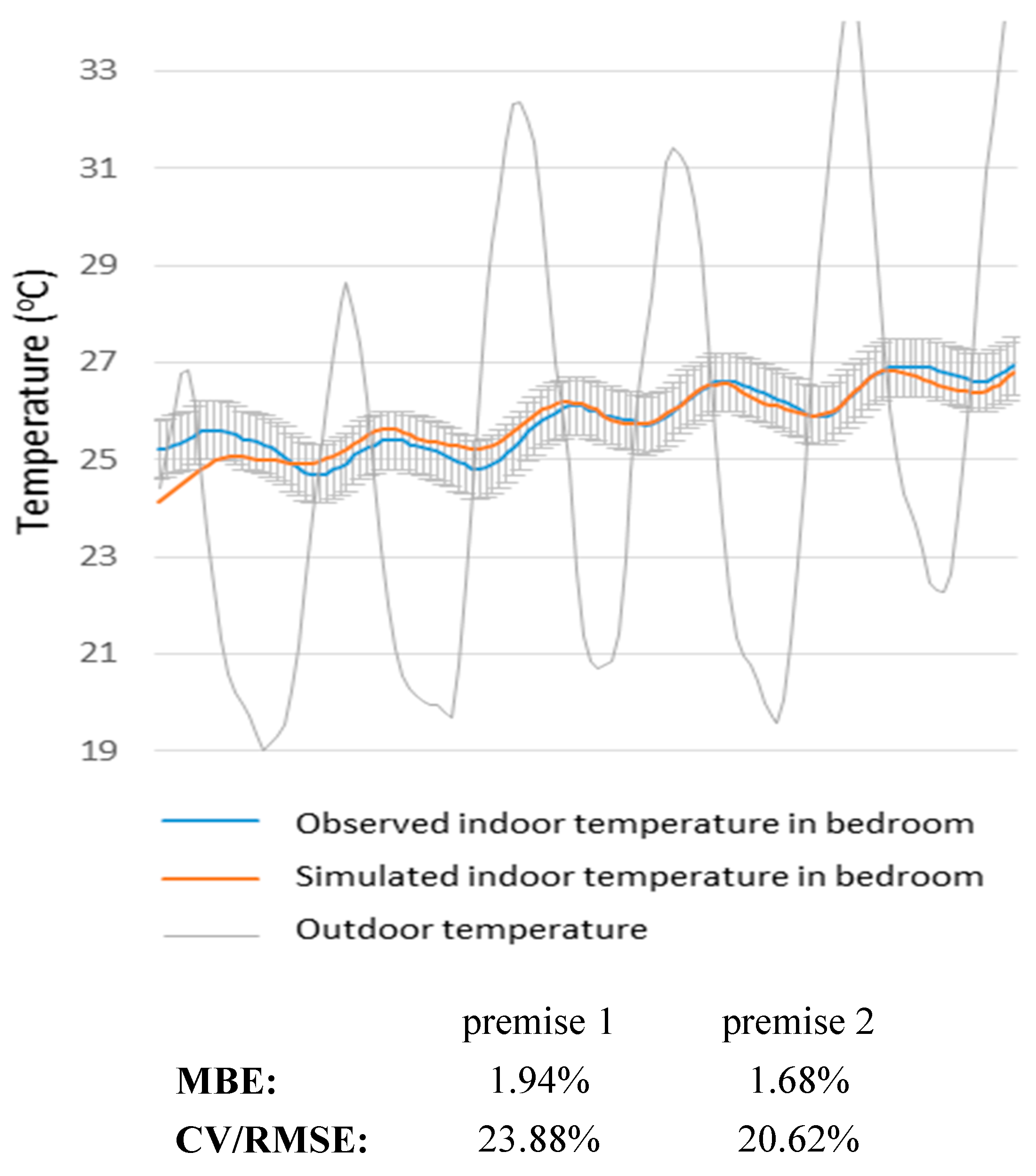
The operating conditions (Table 5) used to simulate the housing units were drawn from the basic procedure for certifying building energy performance in effect in Spain and the energy savings requirements laid down in the country’s technical building code (Annex C, basic document HE: Gobierno de España, 2013 [25]). Those texts define the values for the following indoor parameters: target and control temperature, occupancy, indoor loads, lighting and ventilation.
Operating conditions and occupancy profiles varied with the month of the year and day of the week (weekday or weekend). Spanish legislation envisages night time ventilation of 4 h−1 in the summer months.
Winter was defined as the period from November to March and the rest of the year as summer. Given the importance of climate zone in infiltration-induced energy demand, all five zones were analysed.
The number of times the flats were ventilated, along with the duration and the time of day in winter and summer, were determined for these buildings [38]. The conclusion reached was that the ventilation rate in winter was very low—0.0 h-1 to 0.1 h-1—because windows were opened only minimally in that season. This was supported by findings from a more extensive study conducted by Dubrul [26].

2.2.2. Calibration

The model was calibrated by comparing the values calculated to actual empirical data and adjusting for parameters such as airtightness, density and floor temperature as necessary further to the ASHRAE standard 14-2002 [39] specifications. The control flats were used both to determine thermal behaviour and calibrate the nodal model. Actual thermal and operational profiles were created by extracting hourly values for the indoor parameters as in [40].
Mean bias error (MBE) (Equations (5) and (6)) and the coefficient of variation for the root mean square error (CV/RMSE) (Equation (7)) were used to assess the differences between simulated and observed hourly data:
M B E = i = 1 N s ( y i y ^ i ) i = 1 N s y i
Y S ^ = i = 1 N s y i N s
C V R M S E ( S ) = i = 1 N s ( y i y ^ i ) 2 N s Y ^ S
where
  • y i is the recorded data;
  • y ^ i is the simulated data;
  • N s is the sample size;
  • Y ^ S is the mean recorded data for the sample.
Calibration for model P13 during one week in winter is depicted by way of example in Figure 2, which compares the simulated to the monitored indoor temperature (and ±0.5 °C error). The MBE and CV/RMSE values for both lay within the range defined in ASHRAE 14-2002.

3. Results and Discussion

The sensitivity of building energy performance to building airtightness is discussed below, analysing the response separately for heat gain or loss, i.e., in cooling or heating regimes.

3.1. Overall Impact of Leakage on Energy Demand

The simulated monthly demand values normalised to unit floor area for climate zone B4 graphed in Figure 3 show that heat loss in that zone was attributable more to infiltration than any other factor. Similar findings were observed for the other zones.
The demand values attributable to infiltration are graphed in Figure 4, normalised to unit floor area, for both the cold and warm seasons. One of the most prominent observations was that the effect of air infiltration was most intense in the winter and associated with heating needs. Leakage-related energy requirements in winter were from 10 to nearly 40 times higher than in summer.
Heating demand values associated with leakage rose with the severity of the cold season. The greatest negative balance recorded for all the models was observed in climate zone C3, with a mean of −10.37 kWh/m2, nearly double the mean −5.18 kWh/m2 to −5.8 kWh/m2 observed for the regions with winter climate severity A.
The summertime effect of leakage on demand was much smaller in absolute terms. As a rule, in summer, the negative night-time demand offset the positive daytime demand, lowering the net value or even generating a negative balance. That was observed in areas with milder summers (and night time outdoor temperatures normally lower than the indoor values), such as in climate zone A. The value of such offsets declined with the severity of summer heat (zone 4), with clearly positive balances in the B4 climate zone, for instance.

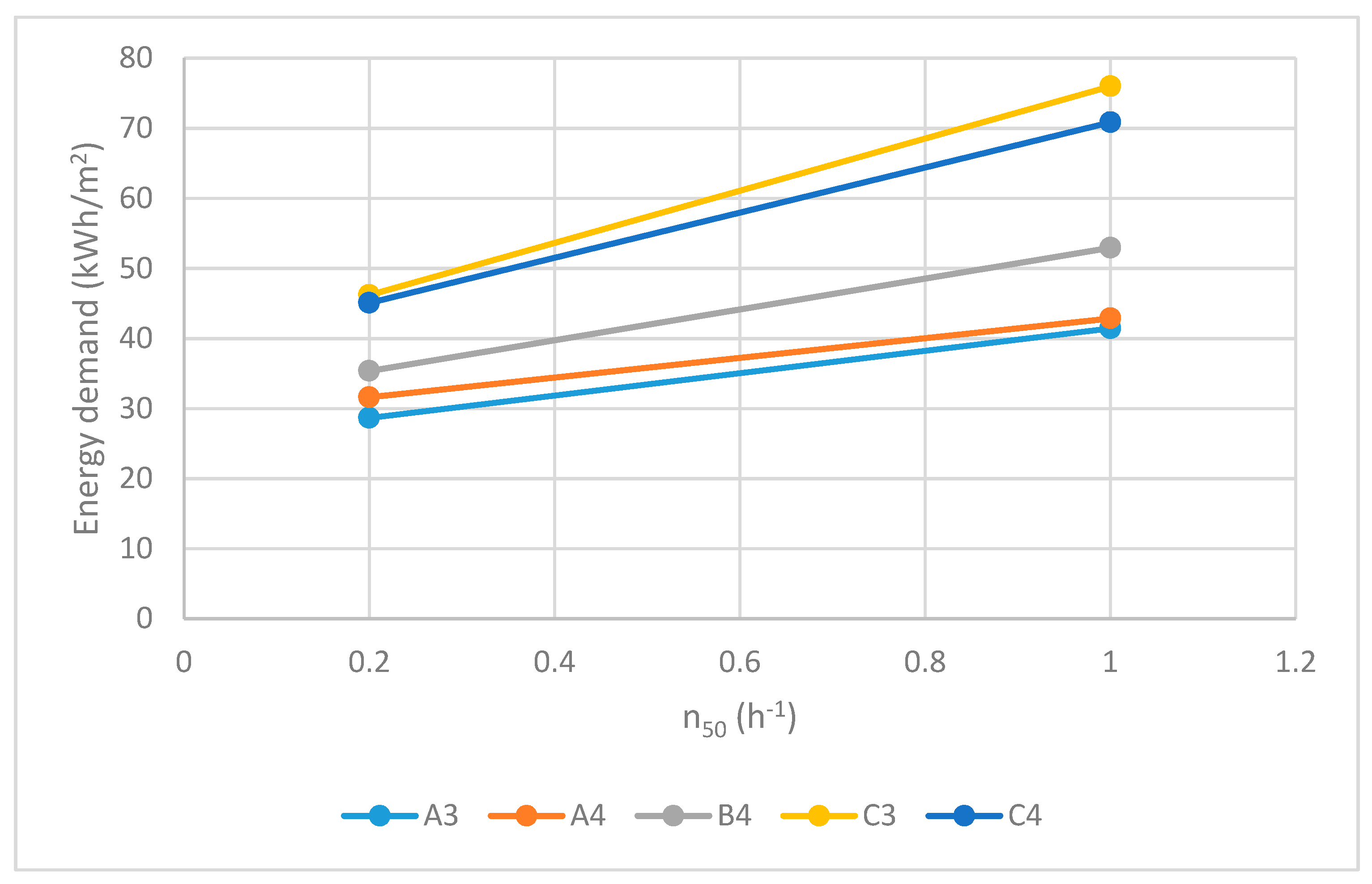
3.2. Energy Demand Sensitivity to Envelope Airtightness

The relative importance of leakage-mediated demand in housing is a variable in the formulation of their cooling/heating load structure. Generally speaking, the models used showed that housing with thermal envelopes best able to control heat flows were the ones that would be most sensitive to changes in air flow rates, i.e., the relative increase in the total load would tend to rise the most where transmission was weakest.
The slope of the curve for predicted demand—ACH rate proposed for each model—was used to determine the variations in cooling/heating loads and the predictions for different leakage values. That procedure holds special promise, for it is directly applicable to predict the improvement potential of envelope rehabilitation.
The correlation between leakage rate and energy demand for a given regime need not necessarily be linear but may exhibit a certain tendency to grow asymptotically after a given ACH value. Nonetheless, in the range normally found in the housing units analysed, it could be likened to a continuous linear relationship. In other words, for the values routinely observed in building stocks, the relationship between infiltration and demand can be fitted to a regression line. The slope on that line is indicative of the relationship between the mean air exchange rate and the expected energy demand, while the other components affecting demand are represented by the constant in the equation. The slopes calculated by simulating housing heating and cooling demand for air changes rate per hour (ACH) of 0.35 h−1 and 0.55 h−1 are discussed below.
The slope values found for infiltration and associated demand leakage rate curves are shown in Figure 5 for the five climate zones analysed. The slopes were flatter in climates with less severe (zone A) and steeper in those with more severe (zone C) winters. The moderate slopes observed for zones A3 (15.97) and A4 (14.08) were an indication that the energy demand in those areas would be less affected by changes in infiltration rate. In contrast, with a slope of 37.23 and a much wider standard deviation, the climate zone C3 sample would be more sensitive to wintertime leakage.
The values published for a similar study on detached housing in Finland [41,42] were higher due to the difference in climate. In this study, with ACH values at around 0.35 h−1, the energy demand ranged from 30 kWh/m2 to 51 kWh/m2 compared to 135 kWh/m2 to 195 kWh/m2 in Finland.

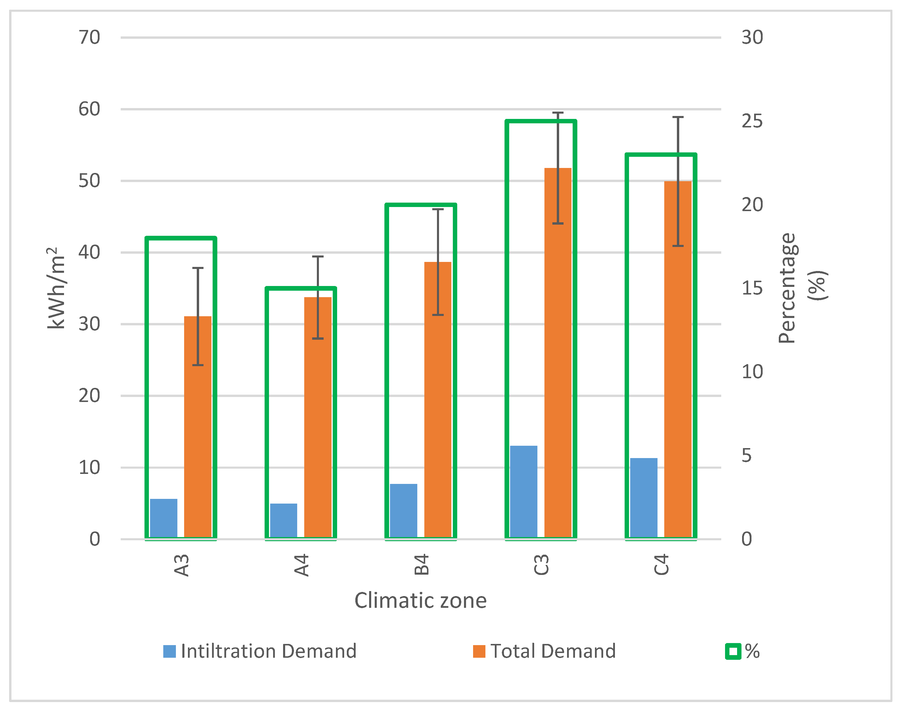
3.3. Predicted Proportion of Demand Attributable to Air Leakage

The model results for mean yearly energy demand attributable to leakage and its relationship to total demand for the climate zones studied, assuming an ACH of 0.35 h−1, are shown in Figure 6.
As in the other values analysed, the peak was observed in climate zone C3, where leakage would account for an annual demand in the order of 13 kWh/m2 or 25% of the total. The lowest values, in turn, were again found for climate zones A3 (with 5.59 kWh/m2 and 18% of the total) and A4 (with 4.93 kWh/m2 and 15% of the total).
Equation (8) is established to predict energy demand for different leakage rates in the building types analysed, delivers a rough estimate for the building stock in the Mediterranean area. The slope, coefficient and standard deviation values are listed in Table 6.
D T O T = m · V 50 20 · V + α
where
  • DTOT is the total energy demand (kWh/m2);
  • m is the slope (value in Table 6);
  • V is the internal air volume (m3);
  • V50 is the air leakage rate at 50 Pa (m3/h);
  • α in the constant (value in Table 6).
This model is valid for social, multi-family housing in climate zones A3, A4, B4, C3 and C4 constructed in 1939–1979. The standard deviation for the slope ranged from 6.5% to 12.1% of the mean, with the highest value observed in climate zone C3 where the highest wintertime demand was also recorded. While the highest absolute standard deviation for the constant was also highest for zone C, the percentage values relative to the mean (18.3% to 23.9%) were in line with those of the other zones, inasmuch as total demand was higher.

4. Conclusions

In this study, airtightness categories were defined by determining and statistically analysing the most prominent variables to establish energy scenarios based on the degree of airtightness in the existing housing stock. The simulations showed building envelope airtightness to be linearly correlated to energy demand at typical n50 values.
They further showed that the correlation between the two parameters followed a similar pattern in all the developments within each climate zone characterised by the same winter severity (A, B or C) because wintertime air permeability was the factor with the greatest impact on energy demand. Its effect was particularly significant in the most severe climates where it was predicted to account for upward of 10 kWh/m2, although values of >5 kWh/m2 were observed in more temperate zones such as A3.
The inference is that infiltration induced 15% to 25% (ACH = 0.35 h−1) of the heating energy demand in typical social housing built prior to Spain’s earliest legislation on building airtightness. In most of the climate zones studied, improving envelope airtightness would translate into a mean potential decline in energy demand of 5% per 0.1 h−1 reduction in the air change rate per hour (ACH), with values of up to 7.2% in the colder areas.
The simulated results delivered by the simplified model described can be used to predict energy demand for the existing housing stock from airtightness values. These parameters should not be interpreted to be constant, however, for airtightness is a variable and, in most cases, a degenerative process. Since much of the housing built to lower standards in the residential stock constituting the population studied here is near obsolescence, identifying the units with the highest potential for alteration of their energy balance due to a decline in envelope quality is particularly appropriate.

Author Contributions

Conceptualization, J.F.-A.; Data curation, J.F.-A., S.D.-A., I.A. and M.Á.C.; Formal analysis, S.D.-A., J.F.-A., I.A. and M.Á.C.; Investigation, S.D.-A., J.F.-A., I.A. and M.Á.C.; Methodology, J.F.-A.; Writing—original draft, S.D.-A., J.F.-A., I.A. and M.Á.C.; Writing—review & editing, S.D.-A., J.F.-A., I.A. and M.Á.C.

Funding

This study was funded by the Spanish Ministry of Economy and Competitiveness under project BIA2012-39020-C02-01, BIA2017-86997-R and the second author benefited from predoctoral contract BES-2013-063097.

Conflicts of Interest

The authors declare no conflict of interest.

References

  1. Healy, J. Housing, Fuel Poverty and Health: A Pan-European Analysis; Routledge: Abingdon, UK, 2017. [Google Scholar]
  2. Gillott, M.; Loveday, D.; White, J.; Wood, C.; Chmutina, K.; Vadodaria, K.; Wood, C. Improving the airtightness in an existing UK dwelling: The challenges, the measures and their effectiveness. Build. Environ. 2016, 95, 227–239. [Google Scholar] [CrossRef]
  3. Johnston, D.; Wingfield, J.; Miles-Shenton, D.; Bell, M. Airtightness of UK Dwellings: Some Recent Measurements. In Proceedings of the RICS Foundation Construction and Building Research Conference, London, UK, 7–8 September 2004. [Google Scholar]
  4. Vinha, J.; Manelius, E.; Korpi, M.; Salminen, K.; Kurnitski, J.; Kiviste, M.; Laukkarinen, A. Airtightness of residential buildings in Finland. Build. Environ. 2015, 93, 128–140. [Google Scholar] [CrossRef]
  5. Paap, L.; Mikola, A.; Teet-Andrus, K.; Kalamees, T. Airtightness and Ventilation of new Estonian Apartments Constructed 2001–2010. In Proceedings of the 33nd AIVC Conference: Optimising Ventilative Cooling and Airtightness for [Nearly] Zero-Energy Buildings, IAQ and Comfort, Copenhagen, Denmark, 10–11 October 2012. [Google Scholar]
  6. Caillou, S.; van Orshoven, D. Report on the building airtightness measurement method in European countries. In ASIEPI: Intelligent Energy Europe; Belgian Building Research Institute: Bruxelles, Belgium, 2010. [Google Scholar]
  7. Chan, W.R.; Joh, J.; Sherman, M.H. Air Leakage of US Homes: Regression Analysis and Improvements from Retrofit. In Proceedings of the 33nd AIVC Conference: Optimising Ventilative Cooling and Airtightness for [Nearly] Zero-Energy Buildings, IAQ and Comfort, Copenhagen, Denmark, 10–11 October 2012; pp. 35–39. [Google Scholar]
  8. Walker, I.; Sherman, M.; Joh, J.; Chan, W.R. Applying Large Datasets toDeveloping a Better Understanding of Air Leakage Measurement in Homes. Int. J. Vent. 2013, 11, 323–338. [Google Scholar] [CrossRef]
  9. Chan, W.R.; Joh, J.; Sherman, M.H. Analysis of air leakage measurements of US houses. Energy Build. 2013, 66, 616–625. [Google Scholar] [CrossRef]
  10. Fernández-Agüera, J.; Domínguez-Amarillo, S.; Sendra, J.J.; Suárez, R. An approach to modelling envelope airtightness in multi-family social housing in Mediterranean Europe based on the situation in Spain. Energy Build. 2016, 128, 236–253. [Google Scholar] [CrossRef]
  11. Fernández-Agüera, J.; Salas, J.J.S.; Medina, R.S.; Domínguez-Amarillo, S. Airtightness and Indoor Air Quality in Subsidised Housing in Spain. In Proceedings of the 35th AIVC Conference “Ventilation and Airtightness in Transforming the Building Stock to High Performance”, Poznań, Poland, 24–25 September 2014. [Google Scholar]
  12. Fernández-Agüera, J.; Sendra, J.J.; Domínguez, S.; Domínguez-Amarillo, S. Protocols for Measuring the Airtightness of Multi-Dwelling Units in Southern Europe. Procedia Eng. 2011, 21, 98–105. [Google Scholar] [CrossRef]
  13. Jesús, F.; Irene, P.; Alonso, G.R.; Cristina, P.; Víctor, E.; Rafael, A.; Jesica, F.; Jesús, D.M.; José, V.; Manuel, M.C.; et al. Methodology for the Study of the Envelope Airtightness of Residential Buildings in Spain: A Case Study. Energies 2018, 11, 704. [Google Scholar] [CrossRef]
  14. Tiberio, A.J.; Branchi, P. A study of air leakage in residential buildings. In Proceedings of the 2013 International Conference on New Concepts in Smart Cities: Fostering Public and Private Alliances (SmartMILE), Gijon, Spain, 11–13 December 2013; pp. 1–4. [Google Scholar]
  15. Infiles Project. Available online: Infiles.uva.es/ (accessed on 27 March 2019).
  16. Sfakianaki, A.; Pavlou, K.; Santamouris, M.; Livada, I.; Assimakopoulos, M.-N.; Mantas, P.; Christakopoulos, A. Air tightness measurements of residential houses in Athens, Greece. Build. Environ. 2008, 43, 398–405. [Google Scholar] [CrossRef]
  17. Alfano, D.F.R.; Dell’Isola, M.; Ficco, G.; Tassini, F. Experimental analysis of air tightness in Mediterranean buildings using the fan pressurization method. Build. Environ. 2012, 53, 16–25. [Google Scholar] [CrossRef]
  18. Alves, S.; Fernández-Agüera, J.; Sendra, J.J. Infiltration rate performance of buildings in the historic centre of Oporto. Inf. Construcción 2014, 66, e033. [Google Scholar] [CrossRef]
  19. Pereira, P.F.; Almeida, R.M.S.F.; Ramos, N.M.M.; Sousa, R. Testing for building components contribution to airtightness assessment. In Proceedings of the 35th AIVC Conference “Ventilation and Airtightness in Transforming the Building Stock to High Performance”, Poznań, Poland, 24–25 September 2014; pp. 322–330. [Google Scholar]
  20. Ramos, N.M.M.; Almeida, R.M.; Curado, A.; Pereira, P.F.; Manuel, S.; Maia, J. Airtightness and ventilation in a mild climate country rehabilitated social housing buildings—What users want and what they get. Build. Environ. 2015, 92, 97–110. [Google Scholar] [CrossRef]
  21. Spiekman, M. The Final Recommendations of the ASIEPI Project: How to Make EPB-Regulations More Effective? Belgian Building Research Institute: Bruxelles, Belgium, 2010. [Google Scholar]
  22. Feijó-Muñoz, J.; Pardal, C.; Echarri, V.; Fernández-Agüera, J.; De Larriva, R.A.; Calderín, M.M.; Poza-Casado, I.; Padilla-Marcos, M.Á.; Meiss, A.; Jesús, F.-M.; et al. Energy impact of the air infiltration in residential buildings in the Mediterranean area of Spain and the Canary islands. Energy Build. 2019, 226–238. [Google Scholar]
  23. Meiss, A.; Feijó-Muñoz, J. The energy impact of infiltration: A study on buildings located in north central Spain. Energy Effic. 2014, 8, 51–64. [Google Scholar] [CrossRef]
  24. Presidencia del Gobierno. Real Decreto 2429/1979, de 6 de julio, por el que se aprueba la norma básica de edificación NBE-CT-79, sobre condiciones térmicas en los edificios. Boletín Oficial del Estado; Gobierno de España: Madrid, Spain, 1979.
  25. Ministerio de Fomento del Gobierno de España, Código técnico de la Edificación (CTE), Spain. 2017. (In Spanish). Available online: https://www.codigotecnico.org/ (accessed on 20 March 2019).
  26. Dubrul, C. Technical Nte AIVC 23. Inhabitant Behaviour with Respect to Ventilation—A Summary Report of IEA Annex VIII; 1988. Available online: https://www.aivc.org/resource/tn-23-inhabitant-behaviour-respect-ventilation-summary-report-iea-annex-viii (accessed on 20 March 2019).
  27. Ferrara, M.; Monetti, V.; Fabrizio, E. Cost-Optimal Analysis for Nearly Zero Energy Buildings Design and Optimization: A Critical Review. Energies 2018, 11, 1478. [Google Scholar] [CrossRef]
  28. Domínguez, S.; Sendra, J.J.; León, A.L.; Esquivias, P.M.; Domínguez-Amarillo, S.; Leon-Rodriguez, A.L. Towards Energy Demand Reduction in Social Housing Buildings: Envelope System Optimization Strategies. Energies 2012, 5, 2263–2287. [Google Scholar] [CrossRef]
  29. Domínguez-Amarillo, S.; Sendra, J.J.; José, I.O.S. La Envolvente Térmica de la Vivienda Social: El Caso de Sevilla, 1939 a 1979 Title, 1st ed.; Editorial Consejo Superior de Investigaciones Científicas: Madrid, Spain, 2016. [Google Scholar]
  30. Domínguez-Amarillo, S.; Sendra, J.J.; Fernández-Agüera, J.; Escandón, R. La construcción de la vivienda social en Sevilla y su catalogación 1939–1979; Universidad de Sevilla: Sevilla, Spain, 2017. [Google Scholar]
  31. Chan, W.R.; Nazaroff, W.W.; Price, P.N.; Sohn, M.D.; Gadgil, A.J. Analyzing a database of residential air leakage in the United States. Atmos. Environ. 2005, 39, 3445–3455. [Google Scholar] [CrossRef]
  32. De La Flor, F.J.S.; Domínguez, S.Á.; Félix, J.L.M.; Falcón, R.G. Climatic zoning and its application to Spanish building energy performance regulations. Energy Build. 2008, 40, 1984–1990. [Google Scholar] [CrossRef]
  33. CEN. Thermal Performance of Buildings—Determination of Air Permeability of Buildings—Fan Pressurization Method; ISO: Geneva, Switzerland, 2015. [Google Scholar]
  34. Fernández-Agüera, J.; Domínguez-Amarillo, S.; Sendra, J.J.; Suárez, R.; Oteiza, I. Social housing airtightness in Southern Europe. Energy Build. 2019, 183, 377–391. [Google Scholar] [CrossRef]
  35. Persily, A.K.; Axley, J. Measuring Airflow Rates with Pulse Tracer Techniques. In STP1067-EB Air Change Rate and Airtightness in Buildings; ASTM International: West Conshohocken, PA, USA, 1990; pp. 31–51. [Google Scholar]
  36. Sherman, M.H. Estimation of infiltration from leakage and climate indicators. Energy Build. 1987, 10, 81–86. [Google Scholar] [CrossRef]
  37. EN 12831:2017. Energy Performance of Buildings. Method for Calculation of the Design Heat Load. Space Heating Load, Module M3-3; BSI: London, UK, 2017. [Google Scholar]
  38. Domínguez-Amarillo, S.; Fernández-Agüera, J.; Sendra, J.J.; Roaf, S. Rethinking User Behaviour Comfort Patterns in the South of Spain—What Users Really Do. Sustainability 2018, 10, 4448. [Google Scholar] [CrossRef]
  39. Ashrae. Ashrae Guide and Data Book (Fundamentals); Ashrae: Atlanta, GA, USA, 2002; p. 148. [Google Scholar]
  40. Raftery, P.; Keane, M.; Costa, A. Calibrating whole building energy models: Detailed case study using hourly measured data. Energy Build. 2011, 43, 3666–3679. [Google Scholar] [CrossRef]
  41. Jokisalo, J.; Kurnitski, J.; Korpi, M.; Kalamees, T.; Vinha, J. Building leakage, infiltration, and energy performance analyses for Finnish detached houses. Build. Environ. 2009, 44, 377–387. [Google Scholar] [CrossRef]
  42. Kalamees, T.; Kurnitski, J.; Eskola, L.; Jokiranta, K.; Vinha, J.; Jokisalo, J. A Comparison of Measured and Simulated Air Pressure Conditions of a Detached House in a Cold Climate. J. Build. Phys. 2008, 32, 67–89. [Google Scholar]
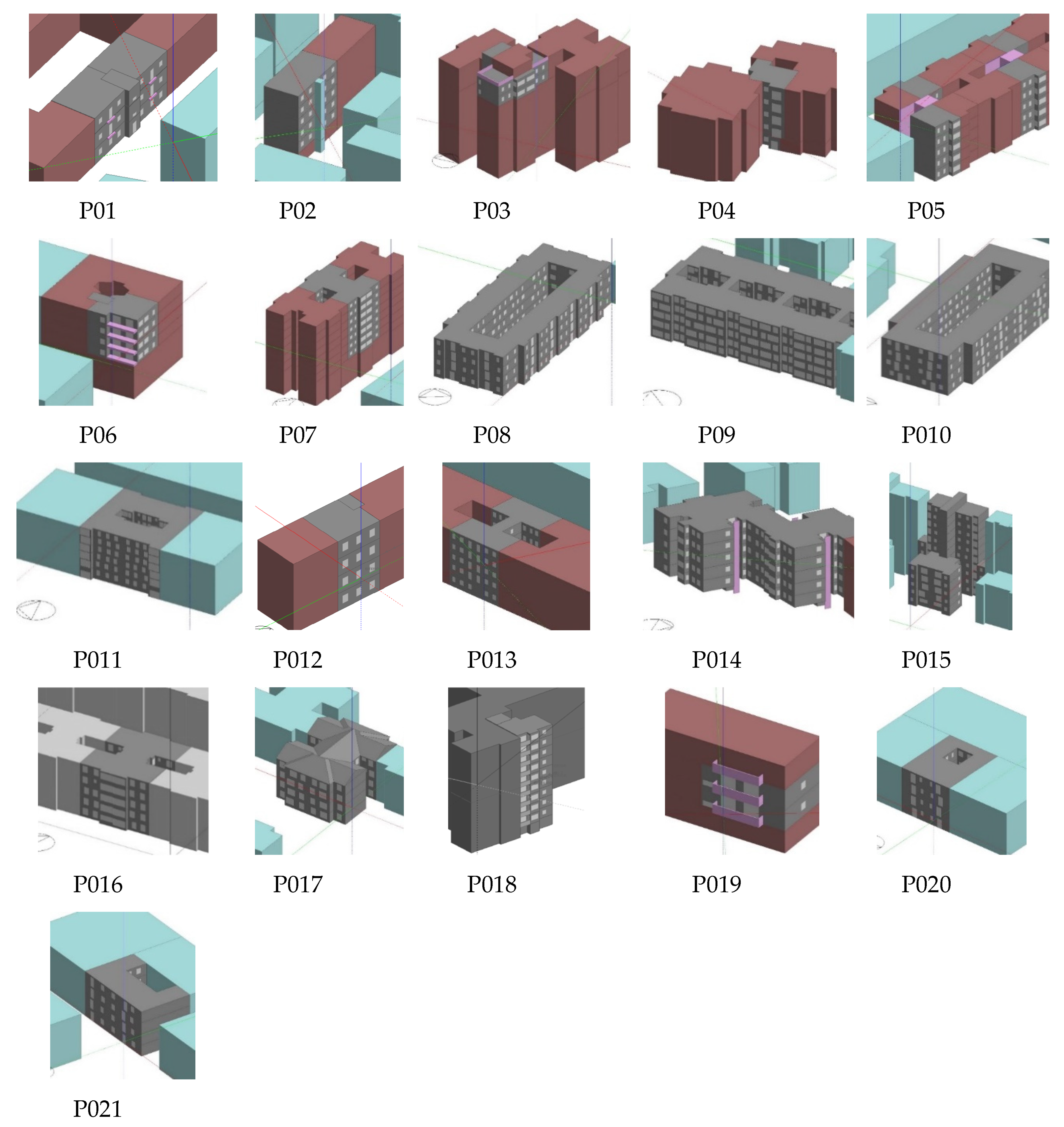
Figure 1. Energy models in the sample studied (Design Builder software).
Energies 12 01677 g001
Figure 2. Comparison of simulated and observed indoor air temperatures (˚C) for model P13.
Energies 12 01677 g002
Figure 3. Predicted heating demand by factor and month in climate zone B4 (ACH=0.35 h-1).
Energies 12 01677 g003
Figure 4. Predicted net demand attributable to infiltration in winter and summer (mean for the climate zones sampled, at ACH=0.35 h-1).
Energies 12 01677 g004
Figure 5. Energy demand vs n50 for five climate zones.
Energies 12 01677 g005
Figure 6. Mean yearly infiltration-induced energy demand (for ACH = 0.35 h−1), yearly mean total demand, percentage of leakage-induced relative to total demand and standard deviation for total demand by climate zone.
Energies 12 01677 g006
Table 1. Year, climate zone and morphological characteristics of sample dwellings.
IDYearClimate ZoneCityFloor AreaVolumeFaçade AreaWindow AreaFaçade Type
(m2)(m3)(m2)(m2)
P011954A3Cádiz6215544101
P021968A3Málaga511313492
P031971A3Cádiz6716137–5382
P041972A3Cádiz641603892
P051974A3Cádiz551384082
P061976A3Málaga10626373142
P071978A3Málaga5112759102
P081966A4Huelva461053862
P091969A4Huelva5714458142
P101970A4Huelva9521251132
P111961A4Huelva451093551
P121951B4Seville461273871
P131963B4Seville581403861
P141964B4Seville59–73161–19979–9209–102
P151965B4Seville4911049132
P161970B4Córdoba531273692
P171973B4Córdoba6415943102
P181978B4Seville7217965192
P191959C3Granada6516267121
P201964C4Jaén561433381
P211967C4Jaén551363872
Table 2. Envelope characteristics.
CompositionTransmittance U (W/(m2K))Solar Factor
FaçadesF1: 1.5 cm cement mortar; 6 inch (11.5 cm) or 12 inch (23 cm) perforated metric brick; 1 cm plaster surfacing 1.56–1.29
F2: 1.5 cm cement mortar; 6 inch (11.5 cm) perforated metric brick; 3 cm to 5 cm non-ventilated air chamber; 5 cm hollow brick; 1 cm plaster surfacing 1.39
Partitions1 cm plaster surfacing; 6 inch (11.5 cm) perforated metric brick; 1 cm plaster surfacing 2.05
Floors/ceilings3 cm tile flooring; 2 cm cement mortar; 25 cm brick infill between one-way beams; 1.5 cm plaster surfacing 1.58
Windows Aluminium frame with no thermal bridge break; single 6 mm glass pane 5.810.82
Table 3. Mean (T), maximum (TM) and minimum (Tm) temperature by climate zone.
Month123456789101112
A3T (°C)12.112.914.716.319.323.025.526.023.519.515.713.2
TM (°C)16.817.719.621.424.328.130.530.828.224.120.117.5
Tm (°C)7.48.29.811.114.218.020.521.118.815.011.38.9
A4T (°C)12.613.315.117.019.723.526.126.724.220.416.413.8
TM (°C)16.917.619.621.424.127.930.531.028.424.520.517.9
Tm (°C)8.39.010.612.515.318.921.722.420.016.312.39.6
B4T (°C)10.912.515.617.320.725.128.227.925.020.215.111.9
TM (°C)16.0 18.121.923.427.232.236.035.531.726.020.216.6
Tm (°C) 5.77.09.211.114.218.020.320.418.214.410.07.3
C3T (°C)6.58.511.413.317.222.325.324.821.116.010.67.6
TM (°C)13.015.419.020.625.031.034.834.229.423.217.013.4
Tm (°C)0.01.63.86.09.413.615.715.512.88.74.21.7
C4T (°C)8.610.313.114.518.223.727.626.922.817.912.39.5
TM (°C)12.114.017.419.023.229.433.732.927.721.915.712.8
Tm (°C)5.16.68.910.013.318.121.421.017.813.88.96.3
Table 4. Blower door test findings for V50, n50 and q50 (mean and standard deviation for each development).
SampleV50 (m3/h)n50 (h−1)q50(m3/hm2)
No. FlatsMeanSDMeanSDMeanSD
1475873.415.130.3917.231.67
231.03844.587.930.3430.531.31
3395489.825.730.5721.202.00
441054198.876.581.0127.745.23
54951142.526.891.0323.783.56
61102503.89014.040
711675013.14028.390
83807296.117.682.8221.247.79
921053447.160.1618.160.76
102651163.010.1312.760.31
1111277011.62036.490
1211294010.12034.050
13388023.516.240.5423.160.62
1441184440.687.321.9214.275.31
1531040174.179.481.5821.223.55
162156413912.31.0943.443.86
1711876011.8043.630
1812624014.68040.370
192830505.110.3112.390.75
204925371.566.462.5928.0311.26
214929226.036.81.6524.455.95
Mean 9851547.51.0425.552.57
Table 5. Operating conditions set out in the basic procedure for certifying building energy performance in effect in Spain and the energy savings requirements defined in its technical building code.
ItemValueTime of Day
WinterSummer
Occupancy 17.8 m2/person 00:00 to 07:00 100%00:00 to 07:00 100%
07:00 to 16:00 25%07:00 to 16:00 25%
16:00 to 23:00 50%16:00 to 23:00 50%
Weekends and holidays: Weekends 00:00 to 24:00 100
00:00 to 24:00 50%Holidays 00:00 to 24:00 0%
Appliances and lighting4.44 W/m2 00:00 to 08:00 10%00:00 to 08:00 10%
08:00 to 19:00 30%08:00 to 19:00 30%
19:00 to 20:00 50%19:00 to 20:00 50%
20:00 to 23:00 100%20:00 to 23:00 100%
23:00 to 24:00 50%23:00 to 24:00 50%
Ventilation4 h-100:00 to 24:00 0%00:00 to 08:00 100%
08:00 to 24:00 0%
Air temperature Target00:00 to 16:00 -00:00 to 08:00
16:00 to 23:00 20 °C08:00 to 23:00 26 °C
23:00 to 24:00 -23:00 to 24:00
Winter: November to March
Summer: April to September
Table 6. Equation (8) parameters used to predict total energy demand from the air leakage rate by climate zone.
Climate Zone Slope (m)Coeff. (α)SDmSDα
A315.9725.471.96.1
A414.0828.791.15.3
B421.9730.972.06.8
C337.2338.764.59.1
C432.2138.642.18.3

