Optimizing the Regulation of Aggregated Thermostatically Controlled Loads by Jointly Considering Consumer Comfort and Tracking Error

Abstract

Thermostatically controlled loads (TCLs) are promising to offer demand-side regulation with proper control. In this paper, the aggregate power of TCLs is used to track the automatic generation control (AGC) signal by changing the temperature setpoint. The dynamics of the indoor temperature are described by a Monte Carlo model, and population dissatisfaction is described by the predicted percentage of dissatisfied (PPD). The objective is optimization from two aspects, minimizing both population dissatisfaction and tracking error. We propose an improved active target particle swarm optimization (APSO) algorithm to optimize the model, making it possible to ensure that the user’s dissatisfaction is as small as possible while the aggregate power tracks the AGC signal. The novelty of this paper is to introduce PPD into the model and at the same time establish three models using PPD as the objective function and constraints. The simulation results are shown to verify the efficiency of the designed model.

1. Introduction

In the traditional power grid, the power system adjusts the output of each generator on the power generation side by automatic generation control (AGC) to maintain the frequency offset within the allowable range [1]. In the process of building a smart grid, frequency adjustment service has become an important issue in the research of power market auxiliary services. Demand-side management (DSM), an aspect of the smart grid, is highly significant for auxiliary grid services [2]. Recently, in the research of demand-side regulation, the direct load control scheme based on air conditioning loads has attracted the attention of researchers due to its fast response speed and low cost [3].

Works such as [4,5] have studied and established a mathematical model based on the physical characteristics of air conditioning load to describe the continuous evolution of the temperature state and the switching process of the thermostat state. In [6,7], a homogeneous air-conditioning load model was described and its synchronization effect and power oscillation were analyzed. Specifically, the influence of the synchronized operation of air conditioning loads and the power of their damage to power system oscillations were studied. In [8,9], the authors established a state queue model for aggregated air conditioning, which proposed a dynamic parameter selection method for the state transition matrix. In [10,11], based on the Markov chain method, the authors established a heterogeneous identification model for the aggregated air conditioning load and analyzed the control performance under different state information. According to the partial differential dissipation model of air conditioning load, a bilinear state space model was established to adjust the temperature setting of the aggregated loads and achieve aggregated power regulation [12]. The control of aggregated air conditioning loads mainly involves two methods: on/off control [13,14,15] and temperature settings adjustment [16,17,18,19]. In [20], the author proposed an adaptive grouping control method for air conditioning loads based on parameter similarity. The authors of [21] designed a random sorting method to control the switching action of air conditioning loads. In [22], the author considered the consumer’s comfort requirements to establish a fuzzy control rule to control the air conditioning load and protect consumers’ demands. Based on the existing switch control methods of air conditioning loads, the authors in [23] designed two methods to introduce the demand response function into the scheduling problem for analysis. In [24,25], an air conditioning load scheduling strategy was proposed based on model reference adaptive control, which can be extended to other load control schemes with similar switching characteristics.

In the above works, the trade-off between population dissatisfaction and power tracking in the power system was not studied. In this paper, three optimization schemes are established to reach a trade-off between population dissatisfaction and power tracking errors by selecting the optimal temperature range for the general public and the grid. The rest of this paper is organized as follows: Section 2 introduces the model of a physically based single thermostatically controlled load (TCL) and a commonly applied thermal comfort model. Section 3 proposes three schemes to reach a trade-off between population dissatisfaction and power tracking errors. Section 4 introduces a temperature setpoint optimization algorithm based on active target particle swarm optimization (APSO), and Section 5 verifies the reliability and rationality of the scheme with MATLAB and EasyFit simulations. Finally, Section 6 summarizes the key contributions of this work.

2. System Model and Problem Formulation

The demand-side regulation system is composed of TCLs, agents, and a control center, as shown in Figure 1. Different numbers of TCLs make up different groups to better provide regulation services for the power system. In addition, the TCLs are common for providing regulation services by indirect load control. In particular, the control center termly transmits control instructions via the temperature setpoints, and the agents turn off and turn on the TCLs according to the AGC signal.

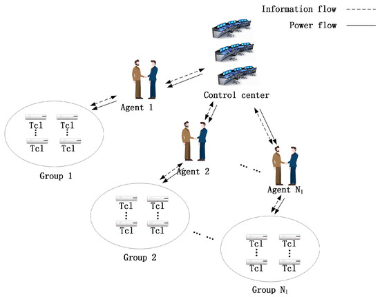
Figure 1. System model.

2.1. Monte Carlo Model

This section introduces a Monte Carlo model to indicate the indoor temperature change of thermostatically controlled loads. We assume that the indoor temperature corresponding to load i ($i=1,2,\cdots ,N$) is $T_i$, and the environmental temperature is $T_{\infty }$. In addition, ${\mathrm{C}}_i$ (kWh${/}^{\circ }$C) and ${\mathrm{R}}_i$ (${}^{\circ }$C/kW) indicate equivalent heat capacity and thermal resistance, respectively. The operating state of a TCL is represented by the variable ${\mathrm{s}}_i$, where ${\mathrm{s}}_i$ = 1 refers to the on state, and ${\mathrm{s}}_i$ = 0 refers to the off state. The cooling power of a TCL is ${\mathrm{P}}_i$ (kW). Then, a separate set of models can be used to simulate the first-order ordinary differential equations for the load dynamics:

$${\dot{T}}_i=\frac{1}{{\mathrm{R}}_i{C}_i}(T_{\infty }-T_i\left(t\right)-{\mathrm{s}}_i{\mathrm{R}}_i{\mathrm{P}}_i),i=1,2,\cdots N.$$

(1)

The on/off state variable ${\mathrm{s}}_i\left(t\right)$ is controlled by the change of temperature deadband:

$$\begin{array}{c}{\mathrm{s}}_i=\left\{\begin{array}{c}0,\mathrm{if}{T}_i\le T_i^{\min },\hfill \\ 1,\mathrm{if}{T}_i\ge T_i^{\max },\hfill \\ {\mathrm{s}}_i,\mathrm{otherwise},\hfill \end{array}\right.\hfill \end{array}$$

(2)

where $T_i^{\min }$ and $T_i^{\max }$ are the lower and upper limits of the indoor temperature, respectively. Furthermore, $T_i^{\min }$ and $T_i^{\max }$ are related to temperature setpoint $T_i^{\mathrm{set}}$:

$$T_i^{\max }=T_i^{\mathrm{sp}}+\frac{\Delta }{2},T_i^{\min }=T_i^{\mathrm{sp}}-\frac{\Delta }{2},$$

(3)

where $T_i^{\mathrm{sp}}$ represents the temperature setpoint of a TCL, and $\Delta$ is the width of the temperature deadband. The aggregated power consumption of TCLs in group l ($l=1,2,\cdots ,M$) can be calculated as follows:

$${\mathrm{P}}_l=\sum _{i=1}^{N_l}\frac{1}{{\eta }_i}{P}_i{s}_i,$$

(4)

where $N_l$ denotes the number of TCLs in group l, and ${\eta }_i$ is the performance coefficient of TCL i.

In the following sections, we assume that the temperature setpoints of TCLs are changed instantly by broadcasting control commands to all TCL units as follows:

$$T_i^{\mathrm{sp}}={\widehat{T}}_i^{\mathrm{sp}}+\Delta T_l^{\mathrm{sp}},|\Delta T_l^{\mathrm{sp}}|\le T_l^{\mathrm{sp},\max }.$$

(5)

In (5), ${\widehat{T}}_i^{\mathrm{sp}}$ is the preferred temperature setpoint of the ith consumer, and $\Delta T_l^{\mathrm{sp}}$ is the command of setpoint change, bounded by $\Delta T_l^{\mathrm{sp},\max }$ for consumer comfort. Therefore, we assume that $\Delta T_l^{\mathrm{sp}}$ is always within the desired range.

Equations (1)–(5) represent the entire Monte Carlo model, which is the basic model for studying TCLs [16,20,26,27,28] and is also the basis for other models. Moreover, the Monte Carlo model is a extensive single-input single-output dynamic model, which will be excellent for the schemes to implement.

The operational characteristics of TCLs over time are shown in Figure 2 and Figure 3. The rising curve indicates the natural temperature rise of the room. An increase in temperature indicates a shutdown of the load. During this period, the system does not consume power, and the room temperature naturally rises due to heat conduction convection. The descent curve represents the cooling process of the air conditioner compressor. The temperature drop indicates the opening of the load, whereby the compressor cooling consumes power and the room temperature decreases. The change in load switch status is closely related to change in room temperature. Once the room temperature arrives at the upper limit, the TCL should be switched on. Once the room temperature arrives at the lower limit, the TCL should be switched off to allow the room temperature to rise naturally.

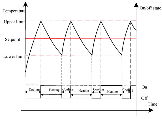
Figure 2. Operational characteristics of a thermostatically controlled load (TCL) when the temperature setpoint is constant.

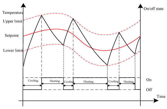
Figure 3. Operational characteristics of a TCL when the temperature setpoint changes with time.

2.2. Predicted Percent Dissatisfied Model

Predicted percentage of dissatisfied forecasts a cluster of people who feel uncomfortable as a percentage of the total number of persons for a given thermal environment according to the average thermal sensation scale. The predicted percentage of dissatisfied (PPD) value is a function of the predicted mean vote (PMV) based people’s voting of thermal sensation in the environment. The unsatisfied people will be reflected by a curve drawn in percentage terms. People’s thermal perception of the environment is different. Even when PMV = 0 in comfortable conditions, there is still that 5 percent of people who are not satisfied.

Thermal comfort plays a crucial role in human comfort. The American Society of Heating, Refrigerating, and Air-Conditioning Engineers (ASHRAE) defines the thermal comfortable environment as being dependent on six variables: air temperature, air velocity, humidity, mean radiant temperature, clothing resistance, as well as activity level [18]. Fanger came up with the thermal comfort equation on the basis of the human body’s heat balance [19]:

$$\begin{array}{c}\begin{array}{cc}{L}_l=\hfill & M_l-W\hfill \\ & -3.05\times {10}^{-3}[5733-6.99(M_l-W)-P_a]\hfill \\ & -0.42[(M_l-W)-58.15]\hfill \\ & -{1.710}^{-5}{M}_l(5867-P_a)\hfill \\ & -0.0014M_l(34-T_{ai})\hfill \\ & -3.96\times {10}^{-8}{f}_{cl}[{(t_{cl}+273)}^4-{(t_r+273)}^4]\hfill \\ & -{f_{cl}{h}_c(t_{cl}-t}_{ai}),\hfill \end{array}\hfill \end{array}$$

(6)

where $L_l$ represents the human body’s heat storage, $M_l$ is the energy metabolism rate of the human body in community l, W indicates the mechanical power of the human body, $t_{ai}$ is the ambient temperature of the bodies of consumers in community l, $t_r$ expresses the indoor average radiant temperature, $f_{cl}$ represents the ratio of clothed surface area to naked body surface area, $P_a$ is the vapor’s partial pressure, calculated taking into account air humidity:

$$\begin{array}{c}\begin{array}{c}{P}_a=\varphi ·\exp [18.956-4030/(t_{ai}+235)],\hfill \end{array}\hfill \end{array}$$

(7)

where $\varphi$ represents air moisture. $t_{cl}$ is clothed body’s mean surface temperature, obtained as

$$\begin{array}{c}\begin{array}{cc}{t}_{cl}\hfill & =35.7-0.028(M_i-W)\hfill \\ & -I_{cl}\{3.96\times {10}^{-8}{f}_{cl}[{(t_{cl}+273)}^4-{(t_r+273)}^4]\hfill \\ & +f_{cl}{h}_c(t_{cl}-t_{ai}),\hfill \end{array}\hfill \end{array}$$

(8)

where $I_{cl}$ indicates the thermal resistance of clothing, and $h_c$ is the convection heat transfer coefficient, which can be expressed as

$$h_c=\left\{\begin{array}{cc}2.38{(t_{cl}-t_{ai})}^{0.25},\hfill & 2.38{(t_{cl}-t_{ai})}^{0.25}>12.1\sqrt{V_a},\hfill \\ 12.1{\sqrt{V}}_a,\hfill & 2.38{(t_{cl}-t_{ai})}^{0.25}<12.1\sqrt{V_a},\hfill \end{array}\right.$$

(9)

where $V_a$ is the air velocity. Combining (6)–(9), we acquire the relationship between room temperature and human body heat storage:

$$L_l=f_2^i{t}_{ai}.$$

(10)

The predicted mean vote (PMV) can be defined as

$${\mathrm{PMV}}_l=(0.303e^{-0.36M_l}+0.028)L_l.$$

(11)

Consumer comfort is usually expressed in PMV. The relationship between PPD and PMV is shown in Table 1. The forecasted dissatisfaction proportion of community i is defined as

$${\mathrm{PPD}}_l=100-95e^{-(0.03353{\mathrm{PMV}}_l^4+0.2179{\mathrm{PMV}}_l^2)}.$$

(12)

Table 1. The relationship between predicted mean vote (PMV), predicted percentage of dissatisfied (PPD), and thermal sensation.

PMV	Thermal Sensation	PPD (%)
+3	Hot	100
−3	Cold	100
−2	Cool	75
+2	Warm	75
+1	Slightly warm	25
−1	Slightly cool	25
0	Neutral	5

3. Optimal Solutions

TCLs are used to provide frequency regulation services to the smart grid and are divided into M groups. Two major goals are proposed: (a) minimization of dissatisfaction, and (b) minimization of error in tracking the AGC signal. Three models are proposed considering comfort constraints and power constraints from three different aspects. The optimized control structure is shown in Figure 4. Within a period t, from $t_0$ to $t_1$, the optimal temperature setpoint ${\mathrm{T}}_i^{\mathrm{set}}$ is calculated, and the control center generates a command, which is broadcasted to the TCLs. TCLS adjust their temperature settings according to the commands.

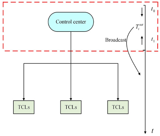
Figure 4. Optimized control structure.

3.1. Scheme A

The objective of this scheme is to minimize the total PPD subject to the power tracking and temperature constraints.

$$\begin{array}{cc}\min \hfill & {\displaystyle \sum _{l=1}^M}{\mathrm{PPD}}_l\hfill \\ \mathrm{s}.\mathrm{t}.\hfill & \left(1\right),\left(2\right),\left(3\right),\left(4\right),\left(5\right),\hfill \\ & |{\displaystyle \sum _{l=1}^M}{\mathrm{P}}_l-{\mathrm{P}}_r|\le \gamma ,\hfill \\ & \Delta T^{\min }\le \Delta T_l^{\mathrm{sp}}\le \Delta T^{\max },\hfill \end{array}$$

(13)

where $\gamma$ is the largest allowable error value, and the error is controlled within $\gamma$, which can meet the required precision value. M is the number of groups of aggregated TCLs, ${\mathrm{PPD}}_l$ is the value of the dissatisfaction of each group, ${\mathrm{P}}_l$ is the aggregated power consumption of each group of TCLs, and ${\mathrm{P}}_r$ is the value of AGC.

3.2. Scheme B

The objective of this scheme is to minimize the largest PPD subject to the power tracking and temperature constraints.

$$\begin{array}{cc}\min \hfill & \left(\max {\mathrm{PPD}}_l\right),\hfill \\ \mathrm{s}.\mathrm{t}.\hfill & \left(1\right),\left(2\right),\left(3\right),\left(4\right),\left(5\right),\hfill \\ & |{\displaystyle \sum _{l=1}^M}{\mathrm{P}}_l-{\mathrm{P}}_r|\le \gamma ,\hfill \\ & \Delta T^{\min }\le \Delta T_l^{\mathrm{sp}}\le \Delta T^{\max },\hfill \end{array}$$

(14)

where ${\max \mathrm{PPD}}_l$ is maximum dissatisfaction in the l groups of consumers.

3.3. Scheme C

The objective of this scheme is to minimize the power tracking errors subject to the PPD and temperature constraints.

$$\begin{array}{cc}\min \hfill & {\displaystyle \sum _{l=1}^M}{({\mathrm{P}}_l-{\mathrm{P}}_r)}^2,\hfill \\ \mathrm{s}.\mathrm{t}.\hfill & \left(1\right),\left(2\right),\left(3\right),\left(4\right),\left(5\right),\hfill \\ & {\displaystyle \sum _{l=1}^{{\mathrm{N}}_l}}{\mathrm{PPD}}_l\le \alpha ,\hfill \\ & \Delta T^{\min }\le \Delta T_l^{\mathrm{sp}}\le \Delta T^{\max },\hfill \end{array}$$

(15)

where $\alpha$ is an upper limit of the total PPD.

We make consumer dissatisfaction the objective function in Scheme A. A smaller degree of dissatisfaction indicates greater comfort for the consumer. From the overall perspective and regarding the sum of dissatisfaction levels of the M groups of TCLs systems as a goal, it is hoped that the consumers’ level of comfort will be relatively satisfactory. In this model, tracking error and temperature setpoint are two constraints. In the whole system, the total power needs to keep up with the reference signal, and the temperature setpoint needs to be controlled within a set range.

Similarly, Scheme B is still from the consumer’s point of view. The objective function becomes that the largest group has the least dissatisfaction. Constraints are the same as Scheme A. We want the power to keep up with the reference signal while the temperature is within the set interval. Compared to the Scheme A, Scheme B focuses more on the satisfaction of a single group of consumers. This can effectively avoid the large differences in PPD values among the groups in the scheme, while the total PPD’s value is still within the acceptable range for the system. However, compared with the first model, this has the disadvantage of large tracking errors and high power consumption.

Scheme C is proposed from the power system side. This model uses the minimum value of the tracking error as an objective function. At this point, the constraints are dissatisfaction and temperature setpoint. The sum of the M groups of dissatisfaction level should be less than $\alpha$, and the temperature needs to be within the set range. Compared with the former two models, the power consumption of this model is greatly reduced, close to the AGC signal, and the power system is more stable. At this time, the power supply is almost equal to the power consumption, but the disadvantage of the system is that the consumers’ dissatisfaction will increase.

To evaluate the tracking performance, the root mean square error (RMSE) is expressed as

$$\mathrm{RMSE}=\sqrt{\frac{{\displaystyle \sum _{k=1}^{N_s}}{e}_k^2}{N_s{(P_{\mathrm{target}}^{\max }-P_{\mathrm{target}}^{\min })}^2}},$$

(16)

where $N_s$ is total number of samples, $P_{\mathrm{target}}^{\max }$ and $P_{\mathrm{target}}^{\min }$ represent the maximum and minimum limits of sample signals, and $e_k$ is the tracking error.

4. Temperature Setpoint Optimization Algorithm Based on APSO

Active target particle swarm optimization (APSO) is a stochastic global optimization algorithm based on a population evolution algorithm [29]. It has the advantages of being a simple algorithm with easy implementation and a good global search ability. At the same time, it has no special requirements for optimizing the form of the objective function. This algorithm has been widely used in many fields such as function optimization, neural network training, parameter tuning, and industrial system optimization. All temperature updates are subject to the following rules:

$$\begin{array}{ccc}\Delta T_j\hfill & =& \omega \Delta T_j+{\mathrm{c}}_1·{\mathrm{rand}}_1·({\mathrm{l}\mathrm{best}}_j-T_j)+{\mathrm{c}}_2·{\mathrm{rand}}_2·(\mathrm{g}\mathrm{best}-T_j),\hfill \\ T_j\hfill & =& T_j+\Delta T_j,\hfill \end{array}$$

where $\Delta T_j$ represents the jth change of temperature, $T_j$ is jth temperature, and ${\mathrm{lbest}}_j$ is the historical optimal value of the jth temperature. $\mathrm{gbest}$ indicates the global optimal value of the entire temperature. The values of ${\mathrm{c}}_1$ and ${\mathrm{c}}_2$ are equal to positive constants, ${\mathrm{rand}}_1$, ${\mathrm{rand}}_2$ are equal to two random numbers from the interval [0, 1], and $\omega$ represents the weighting factor. The temperature setpoint optimization algorithm based on APSO is shown in Figure 5. As an evolutionary algorithm, the APSO algorithm maintains the diversity of the population during the evolution process, which is the precondition for the algorithm to converge to the global optimum. However, when a particle finds a current optimal value, other particles will quickly move closer to it, causing the diversity of the group to be lost, and making the algorithm prone to premature convergence. The whole process is as follows: Firstly, the iteration step size of the temperature range and the temperature change rate is initialized. Secondly, the objective function value is evaluated. Thirdly, the optimal temperature of the individual and the optimal temperature of the group are sought. Fourthly, the update of the temperature and temperature change are implemented, and the objective function value is calculated to determine whether the update condition is satisfied. If it is not satisfied, the temperature and change rate of the temperature continue to be updated. If not, the control center obtains the temperature and change rate of temperature and communicates them to TCLs to provide adjustment services for the balance of the power system. Finally, if the AGC signal meets the termination condition, the service is terminated, otherwise the control center continues to provide AGC load tracking optimization services.

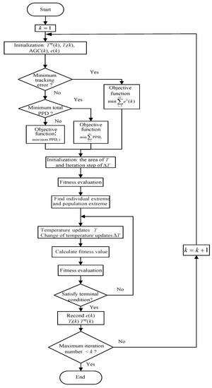
Figure 5. Flow chart of the temperature setpoint optimization algorithm based on active target particle swarm optimization (APSO).

5. Simulation Results

The optimization problem was solved using the MATLAB software platform. The running times of the three schemes were 5 min 26 s, 7 min 3 s, and 4 min 16 s, respectively. The tracking performance of the TCLs under different conditions was analyzed at the same time. In this section, the performances of the global temperature constraints are evaluated through a discussion of three different cases, as well as the trade-off between the dissatisfaction of consumers and the tracking errors. In the three simulation cases, three scheduling indicators were analyzed and compared: one was the tracking error, which reflects the frequency adjustment’s performance, another was the variable room temperature range, which reflects the impact of the requirements of consumer comfort, the last one is the consumers’ dissatisfaction (PPD), which reflects the satisfaction regarding power distribution to the consumer. Each of these three cases was divided into 3 groups ($M=3$ and the total number of TCLs is 3000), of which $N_1$ = 800 in Group 1, $N_2$ = 1000 in Group 2, and $N_3$ = 1200 in Group 3. The number of TCLs is determined by referring to the baseline load value in [30].

TCLs had the parameter values listed in Table 2. We distributed every parameter ($\mathrm{R}$, $\mathrm{C}$, $\mathrm{P}$, $T_{\mathit{sp}0}$, $T_{\infty }$, ${\Delta }_{db}$) normally around the mean value in Table 2. $\mathrm{R}$ and $\mathrm{C}$ obeyed a Gaussian distribution with a mean of 2 and a variance of 0.1. In addition, $\mathrm{P}$ obeyed a mean distribution of 5.6 with a variance of 0.1. A one-hour AGC signal was taken from the Pennsylvania–New Jersey–Maryland (PJM) Interconnection electricity markets, and the sampling time of the signal was 4 s, as shown in Figure 6.

Table 2. Parameter values for the numerical simulations.

Parameter	Value
R Average resistance	2 ${}^{\circ }$C/kW
C Average capacitance	2 $\mathrm{kWh}{/}^{\circ }$C
P Energy transfer rate	14 kW
$\eta$ Load efficiency	2.5
$T_{sp0}$ Initial setpoint temperature	27 ${}^{\circ }$C
$T_{\infty }$ Ambient temperature	32 ${}^{\circ }$C
${\Delta }_{db}$ Thermostat deadband	0.5 ${}^{\circ }$C

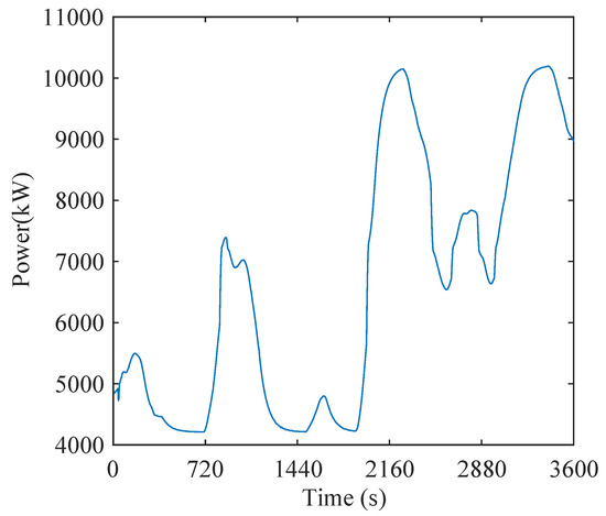
Figure 6. The change chart of automatic generation control (AGC) signals.

As can be seen from Table 3, the total PPD of Scheme A is relatively small, and those of Group 2 and Group 3 are quite different. The total PPD value of Scheme B is relatively large, but the difference between each group is small, indicating that the dissatisfaction is similar across groups. Scheme C was considered from the grid side. In order to make sure the tracking error is minimal, the total PPD is larger.

Table 3. The value of PPD.

	Group	Group 1	Group 2	Group 3	Total
Scheme
Scheme A		6.85%	8.07%	6.24%	21.16%
Scheme B		8.24%	8.72%	7.45%	24.41%
Scheme C		9.86%	11.39%	12.54%	33.78%

In Scheme A, the total PPD is considered as the objective function, the constraints of which are tracking error and temperature. The polymerization properties of the air conditioning load provide service for grid frequency regulation. It can be seen from the data simulation that the total power of TCLs can efficiently follow the sampling signal. Tracking errors are in a small range, and the RMSE reaches 2.44%. We obtain the probability density function of the PPD by using a distribution-fitting software that follows an error distribution with the best fitness:

$$f\left(x\right)=\frac{\alpha k{\left(\frac{x-\gamma }{\beta }\right)}^{\alpha -1}}{\beta {(1+{\left(\frac{x-\gamma }{\beta }\right)}^{\alpha })}^{k+1}},$$

(17)

where k = 1.7182, $\alpha$ = 9.9132, $\beta$ = 8.3863, and $\gamma$ = 0 are the distribution parameters. In addition, the probability density function is shown in Figure 7a.

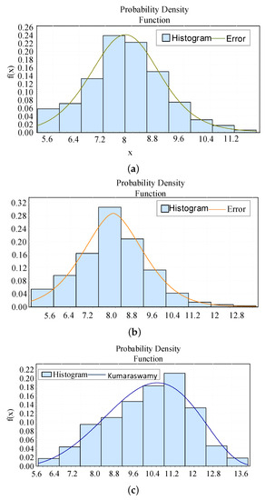
Figure 7. The distribution of the PPD in each scheme. (a) The average value of the PPD in Scheme A. (b) The average value of the PPD in Scheme B. (c) The average value of the PPD in Scheme C.

In Scheme B, the minimum for a single group of PPD is achieved. We also use temperature and tracking error as constraints to evaluate the aggregate properties of the air conditioning load to provide service to the grid frequency regulation. It can be clearly observed that tracking errors are larger than those of Scheme A, and the RMSE achieves 2.65%. We obtain the probability density function of the PPD by using a distribution-fitting software that follows an error distribution with the best fitness:

$$f\left(x\right)=c_1{\sigma }^{-1}exp(-|c_{0}z{|}^k),c_0={(\frac{\Gamma (3/k)}{\Gamma (1/k)})}^{1/2},c_1=\frac{k{c}_0}{2\Gamma (1/k)},z\equiv \frac{x-u}{\sigma },$$

(18)

where k = 1.6664, $\sigma$ = 1.2151, and $\mu$ = 7.9175 are the distribution parameters. The probability density function is shown in Figure 7b.

In Scheme C, the minimum value of the tracking error is considered. It was shown that the tracking errors are smaller than those in Scheme A and Scheme B, and the RMSE achieves 1.37%. We obtain the probability density function of the PPD by using a distribution-fitting software that follows a Kumaraswamy distribution with the best fitness:

$$f\left(x\right)=\frac{{\alpha }_1{\alpha }_2{Z}^{{\alpha }_1-1}{(1-Z^{{\alpha }_1})}^{{\alpha }_2-1}}{(b-a)},wherez\equiv \frac{x-a}{b-a},$$

(19)

where ${\alpha }_1$ = 3.2268, ${\alpha }_2$ = 4.4536, a = 4.4694, and b = 14.879 are the distribution parameters. The probability density function is shown in Figure 7c.

In addition, the setpoint temperature change in the three schemes is shown in Figure 8, from which it is observed that the setpoint changes are within the normal human adaptation range for temperature.

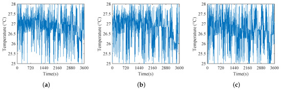
Figure 8. Setpoint temperature change in Scheme A, Scheme B, and Scheme C when N = 800. (a) Setpoint temperature change in Scheme A when N = 800. (b) Setpoint temperature change in Scheme B when N = 800. (c) Setpoint temperature change in Scheme C when N = 800.

Similarly, as shown in Figure 9, the setpoint temperature also follows a continuous distribution. We used the EasyFit software to fit the temperature setpoints of the three schemes and obtain the distribution with the best fitness: the Dagum distribution and the Weibull distribution, which are expressed as:

$$f\left(x\right)=\frac{\alpha k{\left(\frac{x-\gamma }{\beta }\right)}^{\alpha k-1}}{\beta {(1+{\left(\frac{x-\gamma }{\beta }\right)}^{\alpha })}^{k+1}},$$

(20)

$$f\left(x\right)=\frac{\alpha k{\left(\frac{x-\gamma }{\beta }\right)}^{\alpha k-1}}{\beta {(1+{\left(\frac{x-\gamma }{\beta }\right)}^{\alpha })}^{k+1}},$$

(21)

$$f\left(x\right)=\frac{\alpha }{\beta }{\left(\frac{x-\gamma }{\beta }\right)}^{\alpha -1}exp(-{\left(\frac{x-\gamma }{\beta }\right)}^{\alpha })$$

(22)

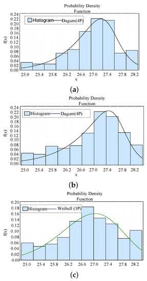
Figure 9. Distribution of the setpoint temperature in Scheme A, Scheme B, and Scheme C when N = 800. (a) Distribution of the setpoint temperature in Scheme A when N = 800. (b) Distribution of the setpoint temperature in Scheme B when N = 800. (c) Distribution of the setpoint temperature in Scheme C when N = 800.

The various parameter values are: for Figure 9a, k = 0.3227, $\alpha$ = 20.392, $\beta$ = 4.5815, $\gamma$ = 22.767; for Figure 9b, k = 0.28468, $\alpha$ = 154.11, $\beta$ = 32.585, $\gamma$ = −5.1572; for Figure 9c, $\alpha$ = 5.2923, $\beta$ = 3.7194, $\gamma$ = 23.26.

For the AGC signal with 900 steps, the switching times of 3000 TCLs under the three schemes are 168, 179, and 158, respectively. On average, the TCL is turned on or off every 5–6 steps. If the time interval between two steps is extended to 60 s, the TCL will be switched 10 times in one hour. In practice, the number of TCLs is larger than 3000. To reduce the switching time of the TCL, we can divide the TCLs into different groups. For example, we divide 60000 TCLs into 20 groups, and each group has 3000 TCLs. In every two-hour schedule, only one group is used. In this way, we can reduce the switching time to one in two hours. It can be seen from Figure 10 that the temperature variables are within the temperature limit. Similarly, Figure 11 shows the tracking performance of the three schemes. It can be seen from Figure 11 that the three schemes can provide promising load tracking services. But the large error in the graph is existed, it is users being picky about comfort that forces a sacrifice in the error to meet their needs. All in all, the load tracking service is still acceptable, which proves that the three schemes are established and reliable. In addition, comparing previous results in Table 4, it is observed that the value of the RMSE is reduced by applying these proposed control strategies.

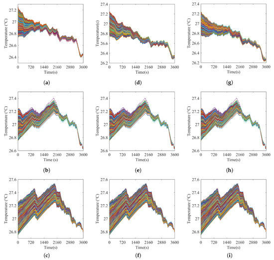
Figure 10. Temperature variation of TCLs in different schemes. (a) Temperature variation of TCLs in Scheme A when N = 800. (b) Temperature variation of TCLs in Scheme A when N = 1000. (c) Temperature variation of TCLs in Scheme A when N = 1200. (d) Temperature variation of TCLs in Scheme B when N = 800. (e) Temperature variation of TCLs in Scheme B when N = 1000. (f) Temperature variation of TCLs in Scheme B when N = 1200. (g) Temperature variation of TCLs in Scheme C when N = 800. (h) Temperature variation of TCLs in Scheme B when N = 1000. (i) Temperature variation of TCLs in Scheme B when N = 1200.

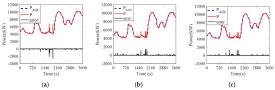
Figure 11. Power tracking results under Scheme A, Scheme B, and Scheme C. (a) Power tracking results under Scheme A when N = 800. (b) Power tracking results under Scheme B when N = 800. (c) Power tracking results under Scheme C when N = 800.

Table 4. Comparison between different control strategies.

PPD Optimal Control Strategies	RMSE
On/off control [31]	20.93%
On/off control with the step rule [30]	17.71%
Setpoint regulation [12]	7.56
Setpoint regulation with ($\rho ,\varphi$) [30]	4.59%
Scheme A	2.44%
Scheme B	2.65%
Scheme C	1.37%

This work fully considers the inherent constraint relationship of frequency adjustment deviation, service cost, and consumer comfort, and achieves an optimal trade-off between power quality cost and consumer comfort in the process of using TCLs to provide frequency adjustment. In contrast to the existing control methods of TCLs, this work also considers the comfort of consumers in the frequency adjustment process, and fairness for the consumers participating in the frequency adjustment service is ensured. The change in actual temperature is from 25 ${}^{\circ }$C to 28 ${}^{\circ }$C, and the corresponding PPD values for each group under the three schemes, as shown in Table 3, show that the scheme has little impact on consumers, indicating that the consumers are willing to participate in the demand response program. RMSE is controlled to be less than 2.5%. Compared with the existing methods in the literature, the method proposed in this paper has higher accuracy, which improves the reliability of the power system.

6. Conclusions

This paper uses a PPD model for expressing consumer dissatisfaction. Three schemes are proposed which consider consumer dissatisfaction and the stability of the grid frequency. The first scheme is proposed to minimize the total PPD of the population. Owing to the large difference in the values of PPD among groups in the first scheme, the second scheme is developed to minimize the PPD of the largest group, in order to achieve PPD fairness for different groups. By considering the power constraints, a scheme of minimizing the tracking error is also proposed. A temperature setpoint optimization algorithm based on APSO is developed to solve the above three schemes and achieve an optimal trade-off between consumer comfort and the cost. It is shown that the proposed schemes can reduce the deviation and cost of TCLs participating in the grid frequency regulation service, ensure consumer comfort, and realize the optimization of frequency regulation deviation, auxiliary service cost, and consumers’ comfort. This establishes a quantitative indicator system for the grid and consumers to assess the cost of participating in ancillary services. The rationality of the model was verified by simulation analysis. The model in this paper can effectively reflect actual factors such as temperature setting and population dissatisfaction. In the future, it would be interesting to study the influence of renewable generation on the results of this work.

References

- Koch, S.; Mathieu, J.L.; Callaway, D.S. Modeling and control of aggregated heterogeneous thermostatically controlled loads for ancillary services. In Proceedings of the Power Systems Computation Conference, Stockholm, Sweden, 22–26 August 2011. [Google Scholar]
- Kirschen, D.S. Demand-side view of electricity markets. IEEE Trans. Power Syst. 2003, 18, 520–527. [Google Scholar] [CrossRef]
- Wai, C.H.; Beaudin, M.; Zareipour, H.; Schellenberg, A.; Lu, N. Cooling Devices in Demand Response: A Comparison of Control Methods. IEEE Trans. Smart Grid 2014, 6, 249–260. [Google Scholar] [CrossRef]
- Ihara, S.; Schweppe, F.C. Physically Based Modeling of Cold Load Pickup. IEEE Trans. Power Appar. Syst. 1981, PAS-100, 4142–4150. [Google Scholar] [CrossRef]
- Chong, C.Y.; Malhami, R.P. Statistical Synthesis of Physically Based Load Models with Applications to Cold Load Pickup. IEEE Trans. Power Appar. Syst. 1984, PAS-103, 1621–1628. [Google Scholar] [CrossRef]
- Kalsi, K.; Chassin, F.; Chassin, D. Aggregated modeling of thermostatic loads in demand response: A systems and control perspective. In Proceedings of the IEEE Conference on Decision and Control and European Control Conference, Orlando, FL, USA, 12–15 December 2011; pp. 15–20. [Google Scholar]
- Sinitsyn, N.A.; Kundu, S.; Backhaus, S. Dynamic Modelling and Control of Heterogeneous Populations of Thermostatically Controlled Loads; University of Newcastle: Callaghan, Australia, 2013. [Google Scholar]
- Lu, N.; Chassin, D.P.; Widergren, S.E. Modeling uncertainties in aggregated thermostatically controlled loads using a State queueing model. IEEE Trans. Power Syst. 2005, 20, 725–733. [Google Scholar] [CrossRef]
- Zhang, Y.; Lu, N. Parameter selection for a centralized thermostatically controlled appliances load controller used for intra-hour load balancing. IEEE Trans. Smart Grid 2013, 4, 2100–2108. [Google Scholar] [CrossRef]
- Liu, M.; Shi, Y. Optimal control of aggregated heterogeneous thermostatically controlled loads for regulation services. In Proceedings of the IEEE Conference on Decision and Control, Osaka, Japan, 15–18 December 2015; pp. 5871–5876. [Google Scholar]
- Mathieu, J.L.; Koch, S.; Callaway, D.S. State Estimation and Control of Electric Loads to Manage Real-Time Energy Imbalance. IEEE Trans. Power Syst. 2013, 28, 430–440. [Google Scholar] [CrossRef]
- Bashash, S.; Fathy, H.K. Modeling and Control of Aggregate Air Conditioning Loads for Robust Renewable Power Management. IEEE Trans. Control Syst. Technol. 2013, 21, 1318–1327. [Google Scholar] [CrossRef]
- Braslavsky, J.H.; Perfumo, C.; Ward, J.K. Model-based feedback control of distributed air-conditioning loads for fast demand-side ancillary services. In Proceedings of the IEEE Conference on Decision and Control, Florence, Italy, 10–13 December 2013; pp. 6274–6279. [Google Scholar]
- Kundu, S.; Sinitsyn, N.; Backhaus, S.; Hiskens, I. Modeling and control of thermostatically controlled loads. arXiv 2012, arXiv:1101.2157. [Google Scholar]
- Perfumo, C.; Kofman, E.; Braslavsky, J.H.; Ward, J.K. Load management: Model-based control of aggregate power for populations of thermostatically controlled loads. Energy Convers. Manag. 2012, 55, 36–48. [Google Scholar] [CrossRef]
- Lu, N.; Zhang, Y. Design Considerations of a Centralized Load Controller Using Thermostatically Controlled Appliances for Continuous Regulation Reserves. IEEE Trans. Smart Grid 2013, 4, 914–921. [Google Scholar] [CrossRef]
- Lu, N. An Evaluation of the HVAC Load Potential for Providing Load Balancing Service. IEEE Trans. Smart Grid 2012, 3, 1263–1270. [Google Scholar] [CrossRef]
- Vanouni, M.; Lu, N. Improving the Centralized Control of Thermostatically Controlled Appliances by Obtaining the Right Information. IEEE Trans. Smart Grid 2015, 6, 946–948. [Google Scholar] [CrossRef]
- Zhang, W.; Kalsi, K.; Fuller, J.; Elizondo, M.; Chassin, D. Aggregate model for heterogeneous thermostatically controlled loads with demand response. In Proceedings of the Power and Energy Society General Meeting, San Diego, CA, USA, 22–26 July 2012; pp. 1–8. [Google Scholar]
- Luo, F.; Dong, Z.Y.; Meng, K.; Wen, J.; Wang, H.; Zhao, J. An Operational Planning Framework for Large-Scale Thermostatically Controlled Load Dispatch. IEEE Trans. Ind. Inform. 2017, 13, 217–227. [Google Scholar] [CrossRef]
- Vivekananthan, C.; Mishra, Y. Stochastic Ranking Method for Thermostatically Controllable Appliances to Provide Regulation Services. IEEE Trans. Power Syst. 2015, 30, 1987–1996. [Google Scholar] [CrossRef]
- Zhang, R.; Chu, X.; Zhang, W.; Liu, Y.; Hou, Y. Fuzzy control design for thermostatically controlled loads considering consumers’ thermal comfort. In Proceedings of the International Conference on Fuzzy Systems and Knowledge Discovery, Xiamen, China, 19–21 August 2014; pp. 165–170. [Google Scholar]
- Yong, T.Y.; Jin, Y.G. Methods for Adding Demand Response Capability to a Thermostatically Controlled Load with an Existing On-off Controller. J. Electr. Eng. Technol. 2015, 10, 755–765. [Google Scholar]
- Liu, M.; Shi, Y. Model Predictive Control of Aggregated Heterogeneous Second-Order Thermostatically Controlled Loads for Ancillary Services. IEEE Trans. Power Syst. 2016, 31, 1963–1971. [Google Scholar] [CrossRef]
- Liu, M.; Shi, Y. Model Predictive Control for Thermostatically Controlled Appliances Providing Balancing Service. IEEE Trans. Control Syst. Technol. 2016, 24, 2082–2093. [Google Scholar] [CrossRef]
- Wu, X.; He, J.; Yin, X.; Jian, L.; Ning, L.; Wang, X. Hierarchical Control of Residential HVAC Units for Primary Frequency Control. IEEE Trans. Smart Grid 2018, 9, 3844–3856. [Google Scholar] [CrossRef]
- Luo, F.; Zhao, J.; Zhao, Y.D.; Tong, X.; Zhang, H. Optimal Dispatch of Air Conditioner Loads in Southern China Region by Direct Load Control. IEEE Trans. Smart Grid 2017, 7, 439–450. [Google Scholar] [CrossRef]
- Yue, Z.; Wang, C.; Wu, J.; Wang, J.; Meng, C.; Li, G. Optimal scheduling of aggregated thermostatically controlled loads with renewable generation in the intraday electricity market. Appl. Energy 2017, 188, 456–465. [Google Scholar]
- Cai, J.D.; Zeng, J.L.; An-Na, L.I. Parameter identification for equivalent circuit of relaxation response based on interval-active particle swarm optimization algorithm. Electr. Mach. Control 2015, 11, 13. [Google Scholar]
- He, H.; Sanandaji, B.M.; Poolla, K.; Vincent, T.L. Aggregate Flexibility of Thermostatically Controlled Loads. IEEE Trans. Power Syst. 2014, 30, 189–198. [Google Scholar]
- Ma, K.; Yuan, C.; Liu, Z.; Yang, J.; Guan, X. Hybrid control of aggregated thermostatically controlled loads: Step rule, parameter optimisation, parallel and cascade structures. IET Gen. Transm. Distrib. 2016, 10, 4149–4157. [Google Scholar] [CrossRef]
© 2019 by the authors. Licensee MDPI, Basel, Switzerland. This article is an open access article distributed under the terms and conditions of the Creative Commons Attribution (CC BY) license (http://creativecommons.org/licenses/by/4.0/).