Performance Optimization of a Kirsten–Boeing Turbine by A Metamodel Based on Neural Networks Coupled with CFD

Abstract

The supply of energy is sustainable only if it is predominantly based on renewable or regenerative energies. For this reason, the use of micro-hydropower plants on rivers and streams is considered recently. This is a particular challenge for the preservation of ecologically permeable streams, so that no dams or similar structures can be considered. While the axial turbine design has prevailed in wind power, there is still no consensus for the generation of energy in free water flow conditions. In this work, an existing prototype of an unusual vertical axis Kirsten–Boeing turbine was investigated. A multivariate optimization process was created, in which all important machine parameters were checked and improved. By using neural networks as a metamodel coupled with flow simulations in ANSYS CFX, a broadly applicable optimization strategy is presented that yielded a blade design that is 36% more efficient than its predecessor in experiments. During the process, it was shown how to set up a complex sliding mesh problem with ANSYS expressions while evaluating a free surface problem.

1. Introduction

The Kirsten–Boeing concept first appeared in the late 1920s as a proposed engine for airships [1]. Since then, parts of its functionality have found their way into modern marine propulsion with the Voith–Schneider [2] propulsion. Apart from that, the use as an omnidirectional turbine for ocean and river currents has not been investigated yet. Compared to other traditional vertical axis turbine concepts, such as Savonius or Darrieus, it combines some advantages of a lift- and a drag-driven rotor in one machine. In addition to being independent of the direction of flow, the turbine does not need start-up aid, but at the same time achieves a higher efficiency than pure drag-driven rotors. It is also conceivable that the turbine is used as a hybrid propulsion system for shipping. Port tugs could navigate with it and charge the batteries when at a standstill. In addition, compared to a Darrieus turbine, it may be more environmentally friendly and less destructive to the underwater world as the Kirsten–Boeing turbine rotates relatively slowly. However, these two considerations are not part of this study.

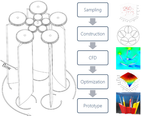
The basic functional principles and the best possible parameter combinations were determined by Computational Fluid Dynamics (CFD). A particular challenge here was the highly asymmetric character of the entire machine. In the numerical model, neither symmetries nor periodic properties of the turbine can be exploited. In addition, stationary solutions have been found to be unreliable due to the massive influence of transient effects and the extensive blade interaction during one revolution, thus time-averaged results of transient CFD simulations have to be used. Finally, a fundamental feature of the turbine makes it difficult to model—each blade has its own axis of rotation in addition to the central machine axis (cycloidal propeller, see Figure 1), which requires the use of custom functions for correct kinematics in ANSYS.

In the end, a final model was generated from the collected experience and parameter combinations, which Was then subjected to a final optimization step. A response surface method was used to determine the optimum blade-profile shape (design of experiments) for the five- and four-bladed machines.

2. The Kirsten–Boeing Turbine

As a cycloidal turbine, the Kirsten–Boeing turbine has the peculiarity that, in addition to the rotation of the machine, the blades also rotate about their own axis at half angular velocity [1]. In this case, the movement is generated by a planetary gearset. Each blade requires two gears to operate the additional rotation. The existing prototype has five blades. A sketch of how it works is shown in Figure 2a. In dangerous situations, it is possible to change the blade pitch (phase angle) in such a way that the turbine comes to a complete halt (indifferent blade position). This can also be used to adjust the machine to any direction of incoming flow (Figure 2b). Due to the vertical construction, most machine components can be installed above the water surface. Furthermore, no additional infrastructure is required for operation, since the turbine operates in free flow conditions, such as in rivers or ocean currents.

An important measure for all turbines is the tip speed ratio $\lambda$, which defines the ratio of circumferential speed u to flow velocity $v_{\infty }$.

$$\lambda =\frac{u}{v_{\infty }}$$

(1)

Due to the fixed kinematics, however, the Kirsten–Boeing turbine is unable to rotate much faster than the surrounding fluid flows. At the twelve o’clock position, the blade is always perpendicular to the flow for a short time, no matter what relative speed between the blade and flow. This leads to low possible tip speed ratios, which in turn requires large blade widths [3]. Those blades cause considerable drag forces in the flow direction, very high material costs and momentum losses, which occur because a particularly large counter-torque is exerted on the outflowing fluid. These losses occur in low $\lambda$-machines because they achieve their power through high torque and low speed [4] (Equation (15)). According to Gasch, this leads to a reduction in efficiency $c_p$ of almost 30% at $\lambda =1$ to ${c_p}_{max}=0.42$. Furthermore, it is to be presumed that, due to the high machine solidity, large separation phenomena occur on the leeward side, which make the blade interaction very complex. Low tip speed machines are thus generally considered economically uninteresting.

3. Validation of the Simulation Environment

Before detailed parameter studies can be carried out, it must be ensured that ANSYS CFX can reliably reproduce the general machine behavior and power output. For this, the complete experimental environment of the prototype is modeled virtually.

3.1. Experimental Environment and Measuring Equipment

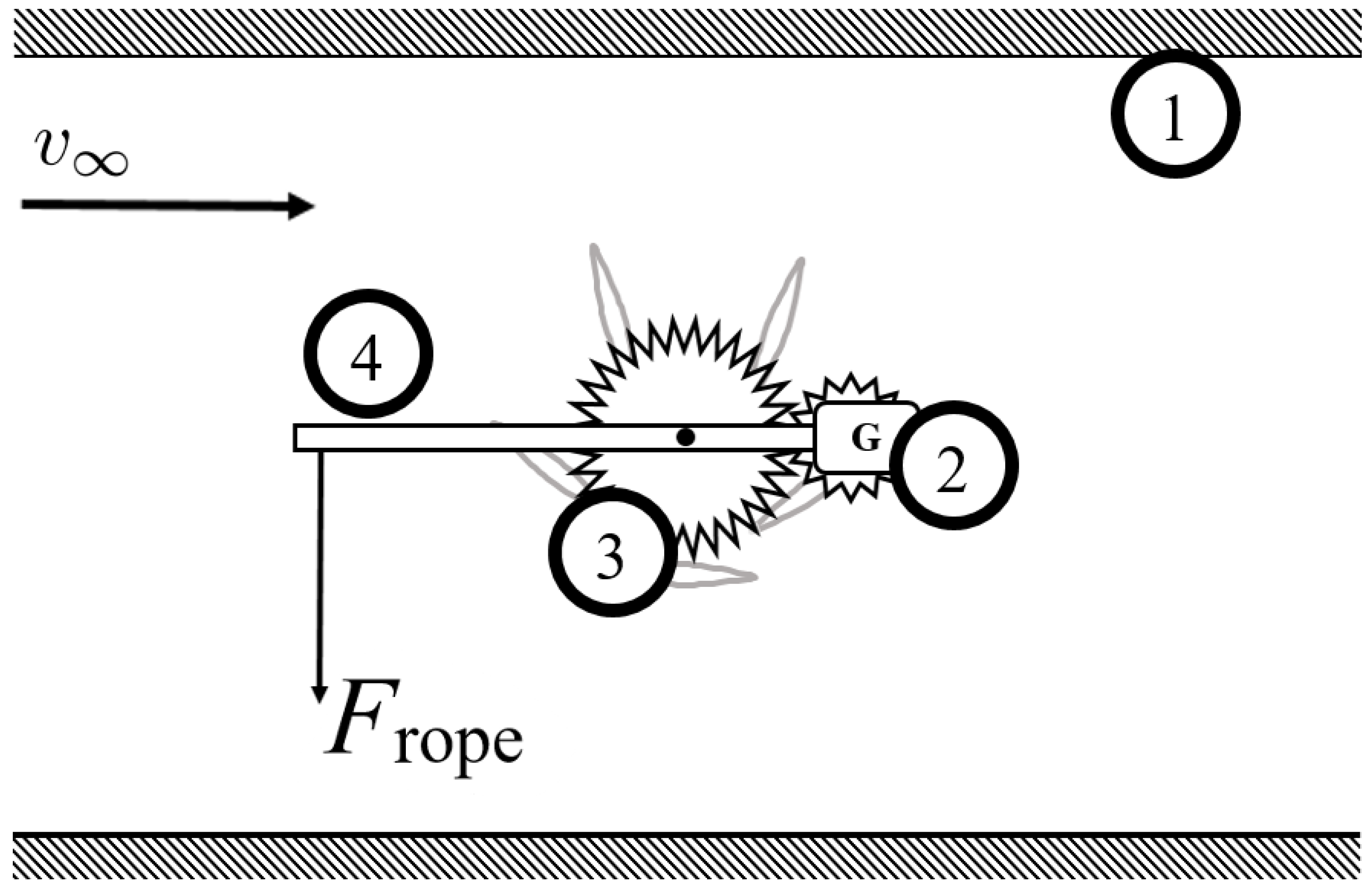
The experiments were carried out in the laboratory of Research Institute for Water and Environment at the University of Siegen (fwu). With a maximum possible volume flow of $Q=150\mathrm{L}\mathrm{s}$⁻¹, flow velocities of approximately $v=0.65\mathrm{m}\mathrm{s}$⁻¹ are achieved. The laboratory water channel has twice the width of the turbine ($0.5\mathrm{m}$) and a depth of $0.7\mathrm{m}$. The length is $25\mathrm{m}$, but was replaced in the simulation by corresponding constraints (see Section 3.5). The task was to find the absolute mechanical power output in relation to the tip speed ratio. To determine mechanical power output $P_{mech}$, the braking torque of a generator was used, which kept the turbine at a constant speed. Consequently, the rotational speed can be adjusted via a variable resistor. The generator itself is freely rotatably mounted so that it translates the turbines torque into a force that lifts a weight on a scale via the rope force $F_{rope}$ (see Figure 3 and Figure A1). From the measured force $F_{rope}$ and the known lever arm l, the acting moment M can be concluded. The product of the turbine rotational speed and torque was the sought after mechanical power.

$$P_{mech}=M·\omega =F_{rope}·l·\omega$$

(2)

The characteristic curve of the machine can be created along by adjusting the variable resistor. The phase angle (angle of rotation of each blade about its own axis) remains constant. All measurements were repeated around 300 times over a period of five seconds and averaged afterwards.

3.2. Structure of the Simulation

The simulation was modeled based on the experimental setup as closely as possible, therefore a multi-phase simulation with air and water was generated. The data for the blade geometry came from the original CAD files of the turbine. It is an axis-symmetric blade with straight flanks and rounded tips (see Figure 4). The geometry creation was followed by the meshing process and the actual setup, which are described below.

3.3. Mesh Independent Solution

The discretization of the fluid domain was carried out in the ANSYS Mesher and allowed a consistent quality of meshing, also for variable geometries and main dimensions. The meshing structure consisted essentially of quad-elements and a prism layer near the wall with a first element offset of $2.5\times 10$⁻⁵ m, which was supposed to resolve the fluid-dynamic boundary layer. The mesh consisted of up to 1,000,000 unstructured hexahedral elements. Since the gap between the blades and the channel floor was neglected (approximately 2 $\mathrm{m}$$\mathrm{m}$), the entire structure could be meshed using a sweep algorithm. At critical points, such as the blade tips, or at domain transitions, the element density was further increased by size functions. In an earlier mesh convergence study, this quality of mesh resolution has proven to be sufficient to generate reliable results in an acceptable time (see Figure 5 and Figure 6).

3.4. Setup–Mesh Movement

The movement of the airfoils was specified by a moving mesh approach a no time consuming recreation of the meshing was not necessary in each time step. As the inner cylindrical domain rotates at the angular velocity $\omega$, the blades also move around their own axis at the velocity $\omega /2$. This behavior could be generated in ANSYS by a subdomain, which assigns a new position to every single mesh node through an expression (function). ANSYS provides the variables X Coordinate, Y Coordinate and Z Coordinate, which can now be moved relative to the node position in the last time step with $\Delta t$. In the following, these variables are summarized in the mesh node vector ${\overrightarrow{n}}_i$. The central domain is rotated by $\phi$ around the Z-axis with the rotation matrix ${\mathit{R}}_z$:

$${\mathit{R}}_z=\left(\begin{array}{ccc}cos\alpha \hfill & -sin\alpha & \hfill 0\\ sin\alpha \hfill & cos\alpha & \hfill 0\\ 0\hfill & 0& \hfill 1\end{array}\right)$$

(3)

$$\phi =\omega ·\Delta t$$

(4)

$${\overrightarrow{n}}_i^{t+1}={\mathit{R}}_z\left(\phi \right){\overrightarrow{n}}_i^t$$

(5)

For the blade nodes ${\overrightarrow{n}}_{i,s}$ ($s=0\dots 5$) a transformation is needed in which the absolute position of the individual blade rotation axis ${\overrightarrow{p}}_s=(x_s,y_s,0)$ for two time steps is calculated. For the calculation in the ANSYS environment, the expression “atstep” (accumulated time step) is used. It outputs the current number of the CFX iteration.

$${\phi }^{t+1}=\mathit{atstep}·\omega ·\Delta t$$

(6)

$${\phi }^t=(\mathit{atstep}-1)·\omega ·\Delta t$$

(7)

The position of each blade axis must also be calculated via expressions. The known blade positions before the simulation $(t=0)$ yields:

$${{\overrightarrow{p}}_s}^{t+1}={\mathit{R}}_z\left({\phi }^{t+1}\right){\overrightarrow{p}}^{s,t=0}$$

(8)

$${{\overrightarrow{p}}_s}^t={\mathit{R}}_z\left({\phi }^t\right){\overrightarrow{p}}^{s,t=0}$$

(9)

$${\overrightarrow{n}}_{i,s}^{t+1}={\mathit{R}}_z\left(\frac{\phi }{2}\right)\left({\overrightarrow{n}}_{i,s}^t-{{\overrightarrow{p}}_s}^t\right)+{{\overrightarrow{p}}_s}^{t+1}$$

(10)

In the event that the phase angle is $\ne 0$, the blade nodes must be initialized with an additional rotation angle ${\phi }_{phase}$. To ensure the stability of the simulation, the additional rotation should be distributed over several time steps. ANSYS offers the use of an IF function depending on the global time step atstep. With the simultaneous conversion to radians for ten iterations follows:

$${\phi }_{phase}=\left\{\begin{array}{cc}0\hfill & ,\mathit{atstep}>10\hfill \\ \frac{2\pi }{360}·\frac{phaseangle}{10}\hfill & ,\mathit{atstep}\le 10\hfill \end{array}\right.$$

(11)

The relative rotation angle $\phi$ can be calculated for a constant angular velocity with $\phi =\omega ·dt$.

3.5. Setup—Domain Properties

From the material library in ANSYS CFX, Water and Air at 25 ${}^{\circ }\mathrm{C}$ were selected at a reference pressure of 101 kPA. Since gravity plays a role, the Buoyancy Model was activated and the gravitational constant was set to $-9.81$ $\mathrm{m}$/$\mathrm{s}$². The reference density for air was $1.2$ $\mathrm{k}\mathrm{g}$/$\mathrm{m}$³, the Ref. Location in the global coordinate system was zero. For multi-phase flow, the Homogeneous Model with the standard Free Surface option was used, meaning the two different phases shared a single velocity field. Heat Transfer was set to 10 ${}^{\circ }\mathrm{C}$ for simplicity, since no significant temperature changes were expected. The surface tension was taken into account by the Surface Tension Coefficient of $0.072$ $\mathrm{N}$$\mathrm{m}$⁻¹ in the Continuum Surface Force model.

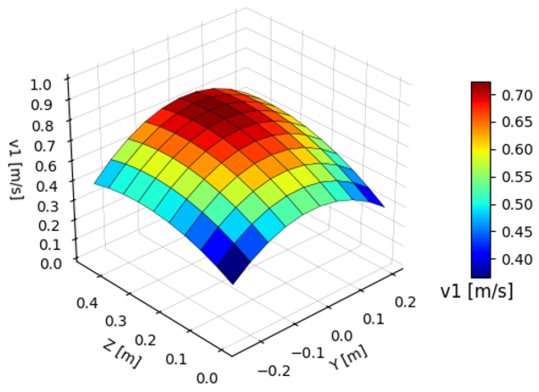
First, a 10-meter-long piece of flow channel was simulated, but, despite the rough side walls, the velocity field was very homogeneous. Since this visually did not seem compatible with reality, and the modeling of the complex inflow into the channel was also not expedient, the velocity field was detected locally by direct measurements. For this purpose, a universal current meter of the type Ott c2 was used 2 $\mathrm{m}$ in front of the turbine. From velocities recorded at a 5 × 5 grid, a function (expression) was generated by using quadratic polynomial regression which, depending on the spatial position (y, z), assigned different entry velocities to the inlet. The x-axis was pointed in the flow direction. The fast core flow, which can be seen in Figure 7, led to a significant change in the turbine performance compared to an erroneously assumed homogeneous velocity. For the entry velocity $v_1$, the function is:

$$v_1(y,z)=-3.84y^2+0.63yz-1.76z^2-0.14y+1.2z+0.51$$

(12)

The determined velocity field was also used to initialize the fluid domain. The air/water state (1, water; 0, air) was initialized with the measurement results for the mean water level height $h_1,h_2$ in front of and behind the turbine, using the following expression:

$$VolFr=\left\{\begin{array}{cc}\left\{\begin{array}{c}1,z<h_1\hfill \\ 0,z>h_1\hfill \end{array}\right.\hfill & ,x<0\hfill \\ \left\{\begin{array}{c}1,z<h_2\hfill \\ 0,z>h_2\hfill \end{array}\right.\hfill & ,x\ge 0\hfill \end{array}\right.$$

(13)

Since only a short area in front of and behind the turbine was simulated but the buoyancy-option was active, the hydrostatic pressure at the boundary conditions had to be taken into account. The outlet had a linearly increasing pressure gradient with the depth z. The equation was also used to initialize the whole domain:

$$P_{Profile}(..)=VolFr·\left\{\begin{array}{cc}\rho g(h_1-z)\hfill & ,x>0\hfill \\ \rho g(h_2-z)\hfill & ,x\ge 0\hfill \end{array}\right.$$

(14)

As a solver, CFX was used with the classic URANS-based SST (Shear Stress Transport) turbulence model [6], which is now the industrial standard and allows reliable results in models affected by strong flow separation. The dimensionless wall distance $Y+$ was $<1$, and the Wall Function option was set Automatic by default. The blade surface was defined as hydraulically smooth, while, for the channel walls, a Sand Grain Roughness of $0.005$ $\mathrm{m}$ was assumed. The resulting Reynolds number was 43,000 ± 1000, while the Froude number for the open channel flow was $0.28$.

For transient time integration, an implicit second-order Euler method was used. Each time step was considered converged if the RMS residuals (Root Mean Square) for momentum and continuity were below $1\times 10$⁻⁴. Between 1 and 15 Coefficient Loops were required. The time step was chosen such that the mesh elements between two domains (sliding interface) in a time step advanced a maximum of half an element further. For $\Delta t=2\pi /\omega N$, besides the angular velocity $\omega$, only the element number N in the circumferential direction (blade domain) must be taken into account. On average, the time step was $0.005$ $\mathrm{s}$ while the total simulation time was about 5 $\mathrm{s}$. Between the static and rotating domains, a transient CFX rotor–stator interface (General Grid Interface) was created to pass over the fluid properties correctly.

3.6. Setup—Performance and Efficiency

The characteristic curve was evaluated at operating points of constant angular velocity. At these operating points, the performance of the turbine was calculated using the following equation:

$$P_T=\omega ·M_T$$

(15)

The final value of the power was averaged over the last revolution of the turbine. ANSYS has the option to apply various operators to variables using Transient Statistics. With <variable>.Trnavg, the arithmetic mean is calculated starting from a specified time step, which can be output directly as a solution variable in the parameter manager. The efficiency of the turbine results from the ratio of the shaft power to the kinetic energy present in the fluid $P_F$ and can be determined by the following equation:

$$c_p=\frac{P_T}{P_F}=\frac{\omega ·M_T}{\frac{1}{2}\rho A{v}_{\infty }^3}$$

(16)

The area A is the “harvesting area” of the machine and $v_{\infty }$ is the mean velocity of the surrounding fluid. The harvesting area was calculated by projecting all blades onto a surface in the flow direction while turning the blades a full revolution. The result was a rectangle with the height of the individual blade and a width that was the doubled distance from the outer most blade tip to the machine centre. All simulations presented in this paper that were to be validated by a physical experiment only outputted the absolute power of the machine. Since the efficiency in the channel flow depends strongly on the ratio of wheel diameter to channel diameter, there would be no generally valid or meaningful value for efficiency. The results of the optimization are given relative to a reference power instead.

3.7. Results of the Simulation

The simulation results are close to the averaged real measurement (see Figure 8 and Figure 9) and the machine behavior could be simulated properly. Due to the low absolute power, however, small interfering factors gained in importance within the experiment. Friction in the bearings, flow around the blade top and bottom (tip losses), blade surface roughness, etc. led to losses that were not shown in the simulation. The deviation from the blue curve at high powers may possibly be explained by the inefficiency of the RANS turbulence model used. At low Reynolds numbers, much of the boundary layer can be laminar, which is not exactly reflected by the classic fully turbulent model. In the real laminar boundary layer, disturbances often led to earlier flow separation compared to a turbulent boundary layer, which increased blade performance and led to problems with the correct calculation of the deep stall [7]. In general, the performance was overestimated, but, since the general machine behavior was well represented, the simulation was still suitable for further optimization of the basic design parameters.

4. Study of the Basic Design Parameters

Currently, there is little experience or conventions for the construction of a Kirsten–Boeing turbine. This study evaluated some basic parameters in terms of their efficiency through 2D flow simulations.

• The optimum number of blades
• Improved blade geometry
• Influence of the blade width

In modern airfoil optimization techniques, correct parameterization is crucial. The method must be able to describe a comprehensive selection of wings with minimal use of geometry parameters. The use of Béziersplines [8] in combination with response surface methods [9] or a Design of Experiments has proven to be particularly efficient. The direct optimization by Evolutionary Algorithms, which also benefit from small parameter sets, is also conceivable.

4.1. Parametric Geometry Creation

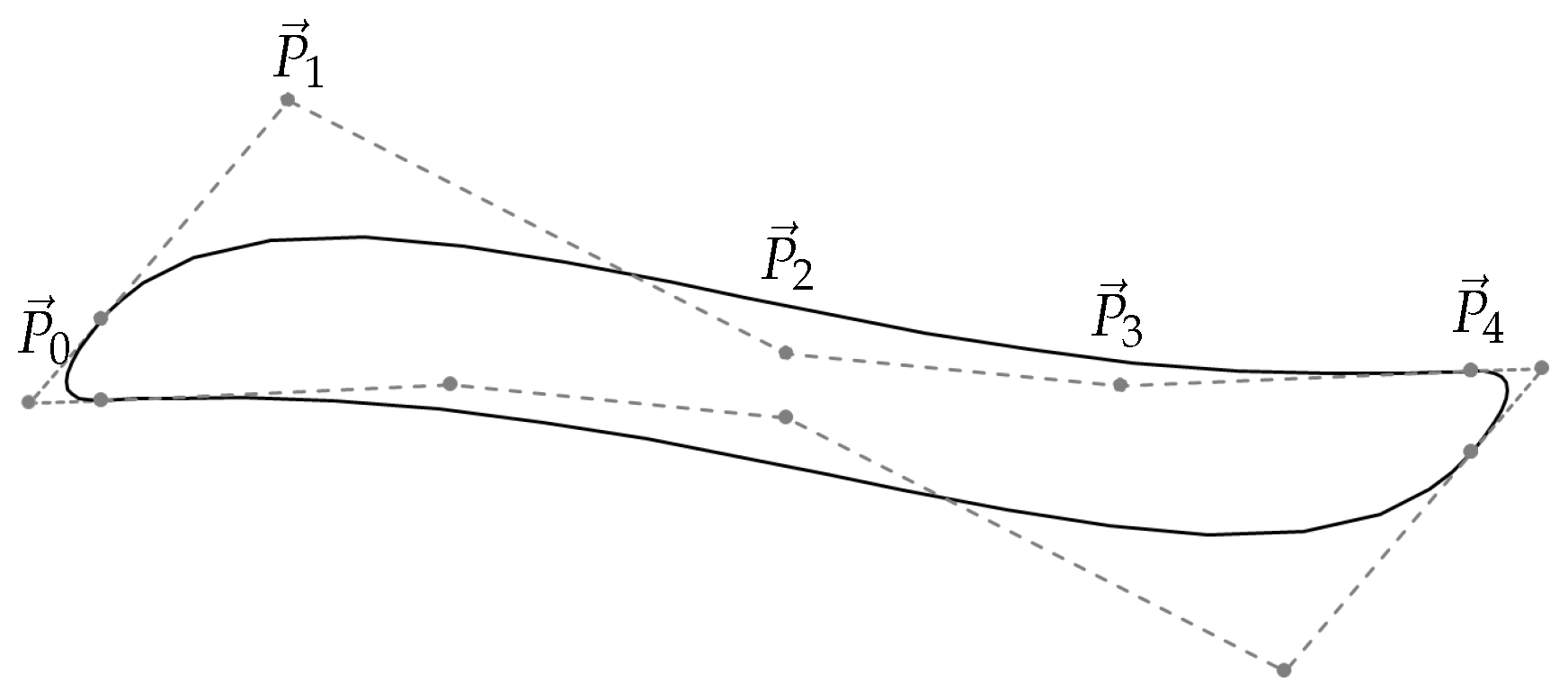
A Bézierspline of degree n is defined by n + 1 support points (${\overrightarrow{P}}_i\mathrm{with}(i=0\dots n)$. In this case, the entire profile consists of two splines (n = 4) on the long flanks, which are connected by two splines (n = 2) at the ends. The so-called Bernstein polynomial is [8]:

$$\left(\begin{array}{c}x\left(t\right)\\ y\left(t\right)\end{array}\right)=\sum _{i=0}^n{B}_{i,n}\left(t\right)·\left(\begin{array}{c}{P}_{x,i}\\ P_{y,i}\end{array}\right)$$

(17)

where the polynomial $B_{i,n}\left(t\right)$ is defined as:

$$B_{i,n}\left(t\right)=\left(\begin{array}{c}n\\ i\end{array}\right)t^i{(1-t)}^{n-i}$$

(18)

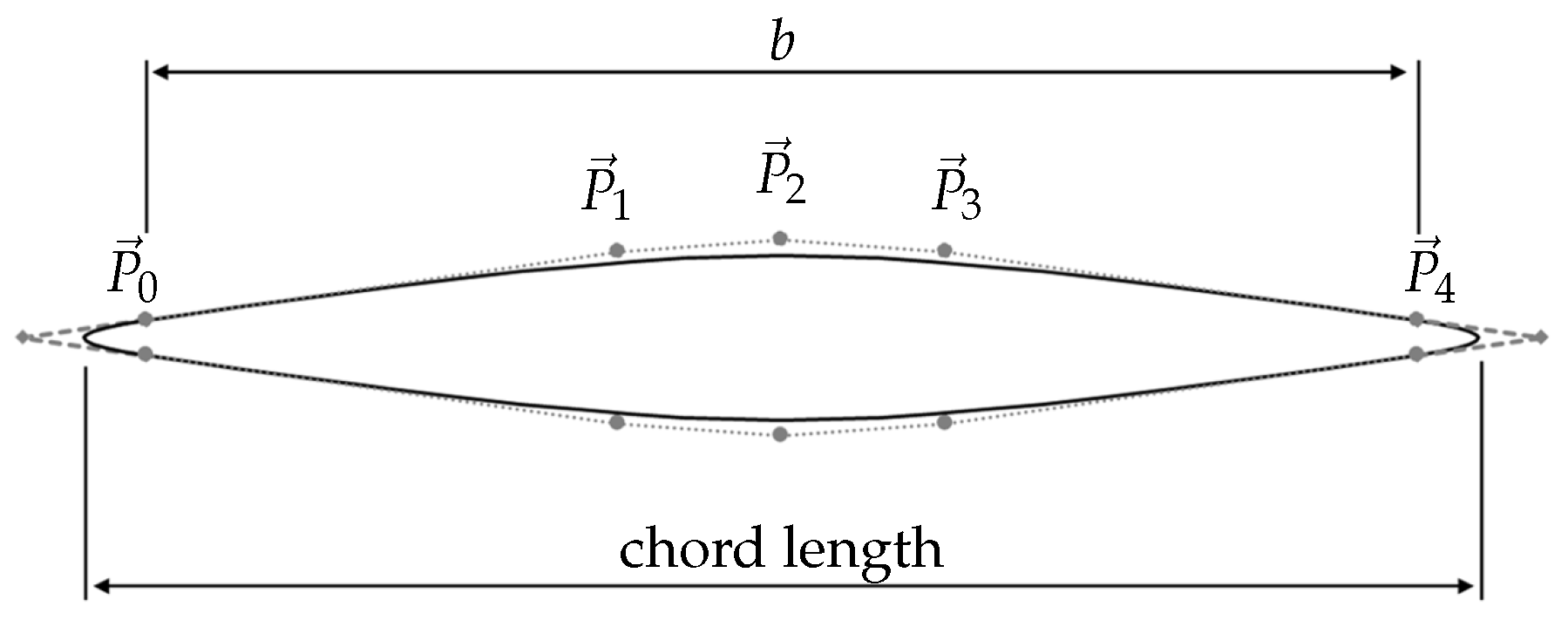
Using the parameter $t=0\dots 1$, any number of point coordinates can now be generated for later use in CAD tools. Because of the symmetry, only two out of four curves need to be defined. The fixed blade width b enforces the position of the outer control points. The number of degrees of freedom continues to be reduced by continuity conditions at the transition between the curves. Since $c_1$-continuity is provided, this leads to the complete definition of the spline at the leading edge. Its center control point ($P_1^2$) lies at the intersection of the tangents with the first points of the two main lines ($\to c_1$). The control point coordinates are shown in

Table 1. Definition of the control points of the upper main spline $n=4$.

i	0	1	2	3	4
$P_{x,i}$	$-b/2$	free	0	free	$b/2$
$P_{y,i}$	free	free	free	free	free

and

Table 2. Definition of the control points of the left short spline $n=2$.

i	0	1	2
$P_{x,i}^2$	$P_{x,0}$	×	$P_{x,0}$
$P_{y,i}^2$	$P_{y,0}$	×	$-P_{y,0}$

. b is a precalculated width variable to make sure the whole blade has the same desired chord length of $0.09\mathrm{m}$ every time. A total of seven free parameters are available. An exemplary profile is shown in Figure 10.

The geometry was parameterized in MS Excel (see Figure 11) and constructed from Béziersplines; the free parameters were initially intuitively assigned. The generated coordinate points can be passed to ANSYS via scripting and converted to true CAD geometry by 3D-Curves in the Designmodeler (by extrusion). In addition, conditions were created in order to be able to easily modify or replace the blade shape on-the-fly. With a machine diameter of $0.5$ $\mathrm{m}$, an outer fluid domain with an extent of 10 $\mathrm{m}$ was created in each direction, which was sufficient to dissipate any transient effects within the domain.

4.2. Setup—Parameter Study

The setup in CFX was the same as the validation calculation, except that the free surface was neglected and the channel wall was removed. After all, the final product should be optimized for free flow. The model was subsequently calculated with only one element over the height. As a result of the significant reduction in the number of elements and complexity, a large part of the calculation time could be saved while increasing the element quality in the plane as well. However, it should be noted that the losses due to the free surface were now neglected and the quasi-2D model generally highly overestimated the actual performance. Nonetheless, the quasi-2D simulation provided meaningful, relative views of different blade configurations, movements and shapes.

To match the flow speeds of real operational locations, the design flow rate $v_{\infty }$ was increased to 1 $\mathrm{m}$ $\mathrm{s}$⁻¹. The default blade profile used a scaled-up version of the first prototype. The performance increased accordingly.

4.3. Optimal Number of Blades

The number of blades significantly determines the material requirements and the complexity of the machine. Each additional blade requires two additional gears in the transmission, which in turn can lead to increased losses due to friction. A high number of blades provides more blade area, but at the same time the influence on each other is stronger. The most efficient option was then found. To ensure a fair comparison, the blade profiles were scaled so that the outer diameter of the turbine remained constant (see Figure 12).

Figure 13 shows the comparison between three, four and five blades with different tip speed ratios $\lambda$. It is striking that the number of blades had a negligible impact on the performance achieved. The high coefficient of performance was due to the nature of the 2D simulations and was not to be considered realistic. For comparison, three additional points in the known 3D configuration were simulated. These showed a drastic reduction in overall efficiency. Real life performance was estimated to be even lower, since in this case the turbine was only simulated in a very wide open channel and the flow could not pass underneath it. Consequently, tip losses were still neglected. It can be noted, however, that fewer blades resulted in larger amplitudes in the torque created (see Figure 14), which may increase the load on the bearings. For example, the maximum fluctuation of the torque on the machine axis with five blades was observed to be 11–18% and for four blades 15–25%. However, the range also depended strongly on the blade shape. The fundamental frequency in the torque curve $f_M$ resulting from rotational speed and number of blades n was:

$$f_M=\frac{\omega }{2\pi }·n\left[Hz\right]$$

(19)

In reality, the effect on the structure was attenuated due to the inertia of the blades and the surrounding fluid. The consequence is that, for the later prototypes, four blades were considered, since they represent a good compromise among achieved power, machine complexity and torque fluctuations. First, however, the existing five-bladed prototype was further developed, as its blades could be easily swapped.

4.4. Optimization of the Blade Profile

Since the turbine is not a conventional purely lift-driven rotor and the blades have to work from both sides, it is not possible to use conventional profile shapes (such as NACA, etc.). Rather, the optimal profile must be found directly in interaction with all other blades. It is not possible to draw any conclusions on the mutual influence of the blades in the back flow region when considering just a single blade (for example, using classic blade element momentum (BEM) theory). Consequently, different blade profiles were simulated and compared as a whole system of five blades. Due to the characteristics of the machine, only axis- or point-symmetrical profiles could be considered. It was likely that thick profiles with a high tolerance to flow separation at high angles of attack would prevail. While the blades rotate in the fluid, they repeatedly increase the angle of attack until the blade is perpendicular to the fluid flow. Thus, the most efficient blade is probably the one that can produce lift forces the longest.

All blade shapes were first used at the optimum operating point of the reference blade. This reference operating point was set at a phase angle of 10${}^{\circ }$ and a tip speed ratio of $\lambda =0.9$. Five blades were used. Since factors such as the free water surface, blade tip losses and losses due to friction were not taken into account, the blade interaction could be seen undisturbed. The result is given in ascending order of the achieved performance (see

Table 3. Performance comparison of different blade profiles.

No.	Profile	max. Power [W]	Relative to Reference (4)
1		74.8	1.17
2		74.4	1.16
3		69.3	1.08
4		64.1	1.00
5		44.6	0.70
6		43.3	0.68
7		26.0	0.41

).

It can be seen that blades with a blunt blade tip tended to be ahead in the simulations. The areas with strong surface curvature increase the flow velocity at this point significantly. According to Bernoulli, a negative pressure is created here, which moves the blade. This flow deflection at the blade tip ensured a favorable distribution of the pressure, such that the resulting force vector almost never pointed to the central machine axis, but deviated from it as far as possible (in the circumferential direction) and thus generated a large torque (see Figure 15). The considerations regarding the profile curvature lad to a profile that had a pronounced rounding at the blade tip. Since only one side of the blade tip is involved in torque generation, point-symmetric blade profiles were considered.

4.5. Influence of the Blade Width

In addition to the profile shape, the absolute width also provides an important parameter. Based on a fixed outer diameter of the machine, there is a maximum allowable blade width where no overlapping occurs. A narrower blade can move further outwards—creating a larger available lever arm. To validate this idea and preserve similitude in flow behavior, the blade profiles were scaled by a simple factor (see Figure 16).

However, as shown in Figure 17, the narrower blades did not reach the performance level of the unscaled blades. Obviously, the effective surface area ess significantly involved in the generation of the total torque. For low tip speed ratios ($\lambda <1$), it is generally assumed that the necessary machine surface area to capture all the flow energy is $>100\%$ of the given flow area [3]. Consequently, the widest possible blade shape was ahead.

5. Metamodel Based Optimization of The Blade Shape

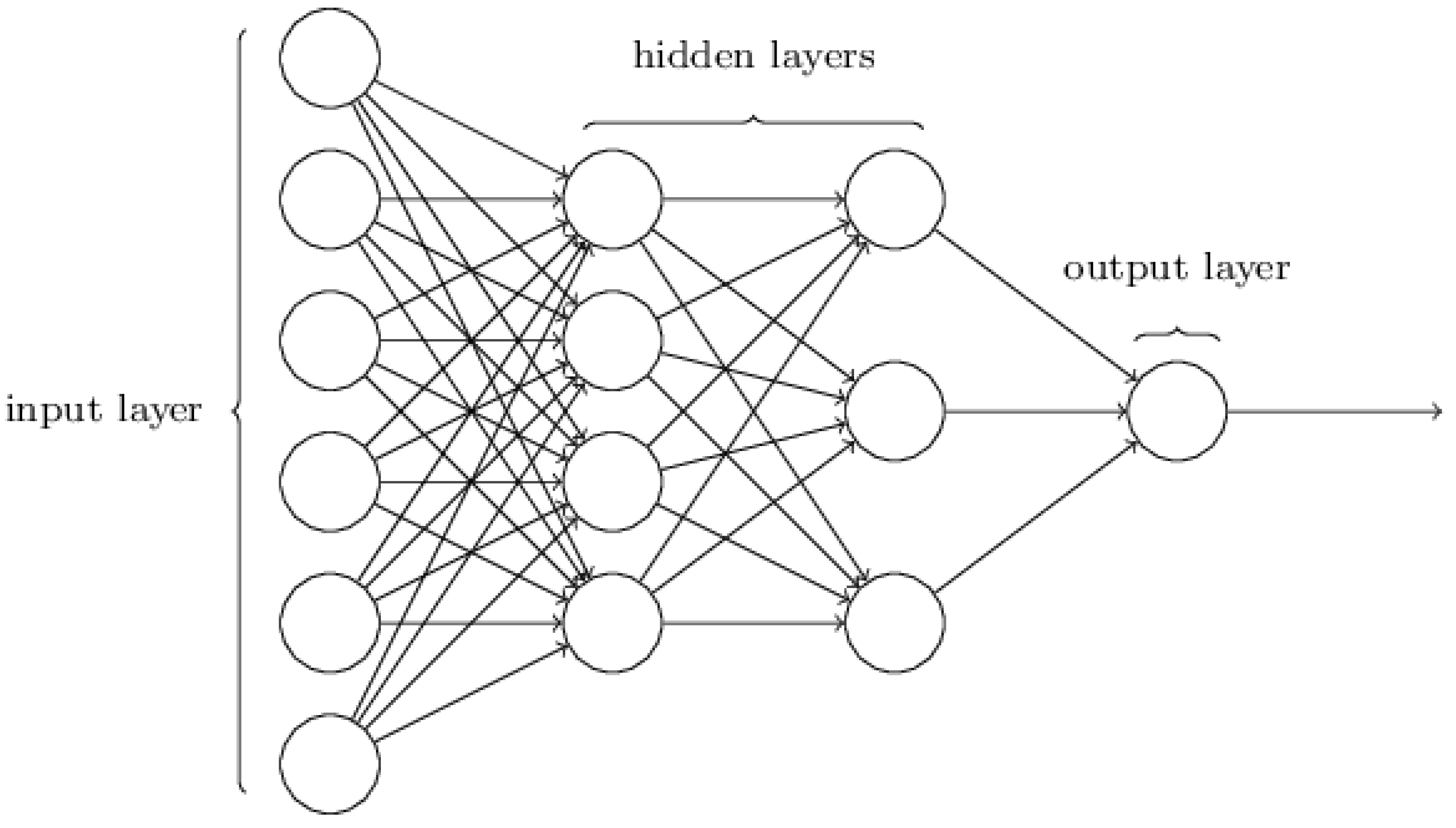
The preliminary investigations showed that a point symmetrical blade shape could lead to higher performances. However, as the optimal parameter configuration was not known for the time being, an automatic optimization process was developed (see Figure 18). The reference profile was still the one used in the validation calculation (see Section 3). The basis for this optimization process was a Multilayer Perceptron (MLP) [10], which is part of the family of deep learning methods. A classic, fully connected feed forward neural network with several layers between input and output was created (see Figure 19). Feed forward here means that the flow of information takes place in one direction only. The net was trained with the usual backpropagation algorithm [11]. As MLPs are increasingly used in the fields of classification, image recognition and approximation, various programming interfaces (APIs) exist that can speed up the training process using a GPU. In this case, TensorFlow [12] was used, controlled by Python scripts.

5.1. Geometry Creation

The structure of the geometry works in much the same way as described in Section 4.1, with the difference that the lower spline is mirrored, creating a point symmetrical blade shape (see Figure 20). To ensure that all possible blade shapes were feasible (no self-intersection), the parameter ranges were manually adjusted and normalized between 0 and 1. There were still seven free parameters preserved. For this investigation, the scale of the smaller prototype based on Section 3 was used again, as it provided the opportunity to manufacture the optimal blade by 3D printing and to experimentally validate it in the laboratory channel.

The network was trained with the data of the flow simulation. For this purpose, 90 different blade configurations were generated and calculated. The resulting metamodel could make predictions in the parameter space known to it. These predictions were used to find the desired maximum within the parameter space, leading to the maximum power, by means of a suitable optimization algorithm.

Sampling used Latin Hypercube Sampling (LHS) because, unlike Monte Carlo sampling, it has no local clusters (Sampling Artifacts) and generally results in better quality results [13]. The samples were evenly distributed in parameter space (Uniform-LHS). Finally, all created designs were numbered consecutively and saved as point coordinates. ANSYS could then script-import all designs serially and convert them into 3D geometry.

5.2. Meshing and Solver

The next steps were the same as in the previous calculations and the simplified quasi-2D setup for the free flow remained unchanged. The operating point to be calculated was still at a phase angle of 10${}^{\circ }$ and tip speed ratio $\lambda =0.9$. After completion of all calculations, the results were split into a training and validation set (80% training, 20% validation), as it must be checked whether the model was sufficiently generalizing and not just memorizing the input data (by over-fitting the model).

5.3. Multilayer Perceptron with Tensorflow

The topology of the neural network was adjusted manually. The best results were provided by a network with three hidden layers, which used rectified linear units (ReLU [14]) as an activation function, each layer having 256 nodes. The default optimization algorithm was Stochastic gradient descent (SGD [11]). As cost function L to be minimized, in contrast to the frequently used quadratic deviation $L\left(a\right)=a^2$, the “Huber loss” function has proven to be particularly effective [15]. Here, a is the difference between prediction and the actual result.

$$L_{\delta }=\left\{\begin{array}{cc}\frac{1}{2}{a}^2\hfill & ,\left|a\right|<\delta \hfill \\ \delta \left(\left|a\right|-\frac{1}{2}\delta \right)\hfill & ,\left|a\right|\ge \delta \hfill \end{array}\right.$$

(20)

where $\delta$ was set to 0.3 in this case. $\delta$ defines the transition at which the piecewise defined cost function changes from the square error to the absolute error. The adjusted loss function reacted less strongly to outliers in the data and led to a better approximation in the validation set. After about 25,000 iterations, there was no further improvement in the loss function of the training or validation set and the calculation was aborted. To measure the quality of the metamodel, a similar method as proposed by OptiSlang [16] was used. Instead of cross-validating and recalculating the metamodel at each input value, however, the formula was applied to the validation set only. The OptiSlang-defined Coefficient of Prognosis (CoP) helped to interpret the values of the cost function.

$$CoP=1-\frac{S{S}_E^{pred}}{S{S}_T}$$

(21)

where $S{S}_E^{pred}$ is the sum of the squares from the error of the prediction, which is divided by the total least squares of the actual solutions to the mean $S{S}_T$. The result is a percentage that describes the predictive quality of the model. In this case, the model reached a quality of about 75%. This method is generally applicable to all regression methods and makes it easy to compare different metamodels. In contrast to the coefficient of determination $r^2$, not all interpolation points that contributed to the construction of the metamodel were taken into account, so that the validity of the prediction quality was much more reliable. Figure 21 shows an example of the resulting response surface of the metamodel for parameter $p2$ and $p5$, while all other parameters were set to $0.5$. The area showed a recognizable optimum for this pairwise parameter combination. To find the actual optimum for all seven parameters simultaneously, a suitable optimization algorithm must be used.

5.4. Particle Swarm Optimization

Since the MLP is a “black box”, it is not easy to know after training where the maximum can be found in the parameter space. Therefore, a simple Particle Swarm Algorithm(PSA) was programmed to do the search. The algorithm is based on the flock behavior of animals in nature and has three main parameters [17]. In addition to the global best position of all particles, each individual knows his own best position. In addition, there is a factor for inertia. After a random initialization in parameter space, each particle moves randomly into each of the n-dimensions ($n=7$). In each time step, the speed is manipulated so that each particle moves in the direction of the currently known global or its local maximum. In addition, the weighting between the two attractions is randomly varied during runtime. The inertia factor and the random weighting should ensure that the particles can also get out of local minima. If a particle exceeds the limits of the parameter space, the value of that dimension is randomly reinitialized.

$$x_{k+1}^i=x_k^i+v_{k+1}^i$$

(22)

$$v_{k+1}^i={\omega }_k{v}_k^i+c_1{r}_1\left(p_k^i-x_k^i\right)+c_2{r}_2\left(p_k^g-x_k^i\right)$$

(23)

• $x_k^i=\mathrm{particle}\mathrm{position}$
• $v_k^i=\mathrm{particle}\mathrm{velocity}$
• $p_k^i=\mathrm{best}\mathrm{individual}\mathrm{position}$
• $p_k^g=\mathrm{best}\mathrm{swarm}\mathrm{position}$
• ${\omega }_k=\mathrm{factor}\mathrm{of}\mathrm{intertia}$
• $c_1,c_2=\mathrm{weighting}$
• $r_1,r_2=\mathrm{random}\mathrm{behavioral}\mathrm{change}$

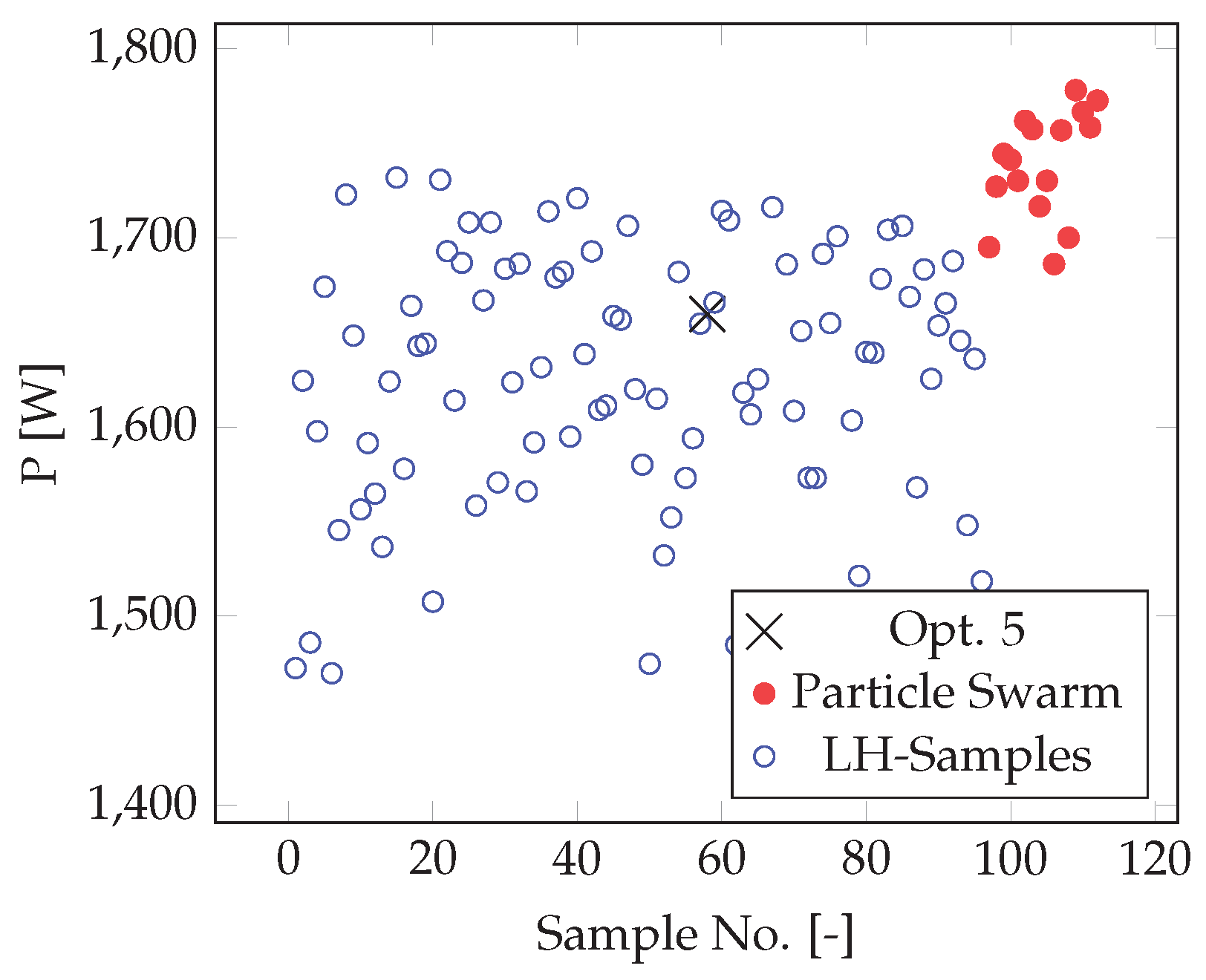
After fine-tuning the $c_1$, $c_2$ and ${\omega }_k$ parameters, a good convergence is achieved after 400 iterations with 100 starting particles. A scatter plot of the individual particle solutions is shown for each iteration in Figure 22.

Once an ideal solution was found, the coordinates are passed to ANSYS and the performance was validated. The process was repeated iteratively and the new values were added to the old training set. After 10–15 iterations, there was no further improvement in the design and the final blade was found. In the simulated 2D free flow, the machine experienced a massive increase of performance of roughly 50% (see

Table 4. Airfoils in comparison from the 2D simulation: Original (1); best sampling (2); and final optimization (3).

No.	Profile	max Power [W]	Relative to Reference
1		8.13	1.00
2		12.01	1.48
3		12.25	1.51

). Because it was not possible in this study to validate the simulation results of the free flow, the optimized airfoils were simulated again as in Section 3 inside the laboratory channel. The channel flow resulted in a simulative performance increase of 32.9%, as shown in

Table 5. Airfoils in comparison in the simulated laboratory channel with free water surface: Original (1); and final optimization (2).

No.	Profile	max Power [W]	Relative to Reference
1		10.22	1.00
2		13.59	1.33

. Thanks to the aerodynamically optimized airfoil shape, the turbine could draw additional power from the much better used lift forces.

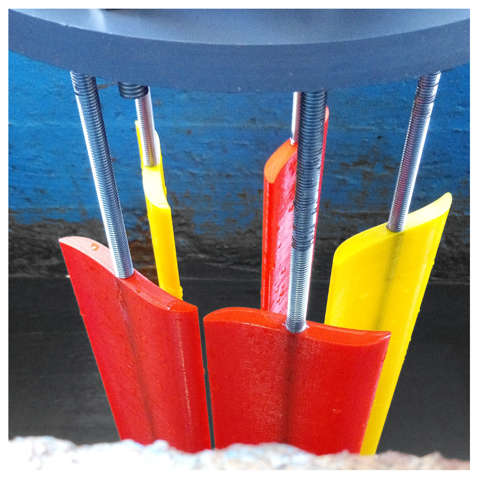
For validation of the simulation results, the original blades on the prototype (see Section 3) were replaced by additively manufactured, optimized blades (see Figure 23). The predicted maximum power increase was also observed experimentally in the confined flow of the channel. A maximum performance improvement of 36.5% for the five bladed prototype was achieved (see Figure 24). While the absolute performance values in the simulation were once again overestimated, the relative increase in performance fit very well with the predictions.

6. Design of the Four Bladed Prototype

Based on the new design rules and determined blade profiles, the optimization process of the final prototype was started. The requirements were a turbine with outer diameter of $1.2$ $\mathrm{m}$ with a vertical length of at least $1.5$ $\mathrm{m}$. Based on the previous findings, the turbines blade number was set to four, while each blade had the maximum possible width. The blades were completely submerged, and, at the optimum operating point, they moved approximately with the flow rate of the water at $\lambda =0.9$. The whole optimization process proceeded again as described in Section 5. Only minor changes were made to cope with the changed machine dimensions.

6.1. Sampling

Since the optimization of the blade shape had previously only been done for a small five-blade machine, it was required to repeat the same steps for the large four-blade variant. The default profile for the new optimization was the previously determined best variant, because it could be assumed that the new optimum was close to the old one in parameter space. The individual parameter ranges were normalized again between 0 and 1 and the actual values were adjusted so that only functioning blade designs were created (for example, no overlapping of the splines; see Figure 25). When sampling the new parameter variations, the old, upscaled design was placed exactly in the middle of the new parameter space so that the average value ($0.5$) for all free variables resulted in the original design. In total, 102 unique blade designs were generated using the known uniform Latin Hypercube Sampling (uLHS).

6.2. Meshing and Solver

The quasi-2D model now consisted of approximately 500,000 unstructured tetrahedral elements (see Figure 26). To approximate the actual environmental conditions at the site of future measurements and experiments, the flow velocity $v_{\infty }$ at the inlet was increased to $1.4$ $\mathrm{m}$$\mathrm{s}$⁻¹. The total torque was determined for a virtual blade length of $1.5$ $\mathrm{m}$.

6.3. Results of the Optimization

After calculating all 102 samples, the averaged torque of each was passed to the MLP. The topology remained unchanged. Finally, when the evaluation of the loss function showed no further improvement, the training of the neural network was stopped. The quality of the metamodel was again described by the CoP value (see Section 5.3) and was now $79.1\%$. Next, the Particle Swarm Algorithm generated different suggestions for new parameter configurations that were validated in CFX (Figure 27). Figure 28 shows the initialization and movement of particles in parameter space in two dimensions. Since the search in the background actually worked in seven dimensions, the particles were apparently able to leave the response surface and find an optimum near 1800 $\mathrm{W}$. In contrast to the algorithm described in Section 5.4, the particles were not randomly reinitialized when the permissible range was exceeded, but they bounced in the opposite direction at twice the speed. However, this change had mainly advantages in the visualization and did not add any significant advantage in the speed of convergence. The last result of each search was computed in CFX, added to the set of training data, and the neural network was trained again on several hundred iterations. After the last five variations were very close to each other, the optimization process was stopped (see Figure 28).

The final blade design achieved a performance of $1772.5$ $\mathrm{W}$, which was 6.8% more efficient than the optimum of the design actually developed for the five-blade prototype ($1659.7$ $\mathrm{W}$). Notable was the increased curvature of the profile top, as shown in Figure 29. Highly curved profiles are used in aircraft designs for slow-moving aircraft, which require a high lift coefficient. The increased lift could probably also be converted into additional energy in the turbine. The large leading edge radius on the front also provided an improved flow separation behavior [18], thus the blade had more time to generate lift during its continuous turning.

Figure 30 shows that only the front of the turbine that is facing the flow was involved in the actual power generation. On the back side of the machine, the blade pitch in combination with the passage through the detached flow led to a significantly negative torque contribution. This undesired effect is a fundamental issue. A low tip speed ratio in vertical axis machines led to a large blade width that blocked the flow through the machine itself and created larger areas of detached flow. The effect worsened for the Kirsten–Boeing turbine design when the angle of attack was tweaked by the ${\phi }_{phase}$ parameter. Because of the global nature of that specific mechanism, all blades were turned either clock- or anticlockwise at once, which resulted in an increased angle of attack on one side of the machine, while the angle on the other side decreased. The negative angle of attack yielded a negative torque contribution. However, since less energy was converted on the leeward side due to the large area of detached flow, there was nevertheless a net advantage for the adjustment of the blade angle.

7. Conclusions

To solve a variety of optimization problems related to the Kirsten–Boeing turbine, comprehensive 3D flow simulations were made in ANSYS CFX. The tests included a general study of all parameters of the turbine, such as the number of blades, blade width and the optimization of the blade profiles themselves. It was found that the number of blades only plays a subordinate role in terms of performance. However, due to the low tip speed ratio, the blade width should be designed as large as possible. Through this realization, the structure of the turbine has changed fundamentally, since now four instead of five blades can be used. In addition to a slightly higher power output, this design also results in significantly reduced material consumption since fewer blades also mean fewer gears and bearings in the gearbox.

After calculating some intuitively hand-made blade designs, it was found that blade tip curvature has a significant impact on the more efficient use of lift forces. As part of these considerations, a point symmetric blade design was set up parametrically to serve as a blueprint for a large number of similar blades. The possibility to freely modify the blade shape allowed identifying and optimizing relevant parameters by means of statistical experimental design. From several hundred randomly generated blade designs calculated in CFX, neural networks were used to generate a metamodel. Within the higher-dimensional response surface given by the model, it was possible to find an optimum with a simple Particle Swarm Algorithm, which is superior to all previous blade designs. Overall, a substantial and validated performance increase of nearly 36% was achieved in the laboratory channel. The optimization process shown here can also easily be applied to similar problems, be it the optimization of individual profiles or entire machines.

The machine efficiency could not be validated in free flow conditions. However, the performed 3D simulations and the experiments in the laboratory channel hinted at an efficiency of 25–30% (see Section 4.3). This means that the Kirsten–Boeing turbine is positioned between the two other vertical axis turbines, Savonius ($c_{p,max}=0.15$) and Darrieus ($c_{p,max}=0.4$ [19]), in terms of efficiency. In terms of complexity, it is above the alternatives, which in addition to the high production costs also means difficulties in scaling to large diameters. When the overall machine diameter is increased, the blade weight increases significantly faster than with a comparable Darrieus turbine. It has been shown nevertheless that CFD is a suitable tool for simulating and optimizing even complex turbomachines where transient effects are decisive. However, due to the fundamentally limited efficiency of the design itself, the economical use of a Kirsten–Boeing turbine remains unlikely.

References

1. Sachse, H. Kirsten-Boeing Propeller; Technical Report; National Advisory Committee for Aeronautics: Washington, DC, USA, 1926.
2. Voith. Schaufelrad mit beweglichen Schaufeln. Available online: https://patents.google.com/patent/DE500340C/zh (accessed on 13 March 2019).
3. Miller, R.H. Energietechnik und Kraftmaschinen 6, Techniklexikon; Rowohlt Taschenbuch-Verlag: Hamburg, Germany, 1972. [Google Scholar]
4. Gasch, R.; Twele, J.; Bade, P.; Conrad, W.; Heilmann, C.; Kaiser, K.; Kortenkamp, R.; Kühn, M.; Langreder, W.; Liersch, J.; et al. Auslegung von Windturbinen nach Betz und Schmitz; Vieweg+Teubner Verlag: Wiesbaden, Germany, 2005. [Google Scholar]
5. Jensen, J.; Wieland, J.; Schmidt, J.; Metzger, J.; Stiller, H.L. BMWi-Projekt StEwaKorad; Technical Report; Lehrstuhl für Hydromechanik, Binnen- und Küstenwasserbau: Siegen, Germany, 2016. [Google Scholar]
6. Menter, F. Two-Equation Eddy-Viscosity Turbulence Models for Engineering Applications. AIAA J. 1994, 32, 1598–1605. [Google Scholar] [CrossRef]
7. Lanzafame, R.; Mauro, S.; Messina, M. 2D CFD Modeling of H-Darrieus Wind Turbines Using a Transition Turbulence Model. Energy Procedia 2014, 45, 131–140. [Google Scholar] [CrossRef] [Green Version]
8. Bezier, P. Numerical Control; Mathematics and Applications; John Wiley and Sons Ltd.: Hoboken, NJ, USA, 1972. [Google Scholar]
9. Box, G.; Draper, N. Empirical Model-building and Response Surfaces; John Wiley and Sons Inc.: Hoboken, NJ, USA, 1987. [Google Scholar]
10. LeDell, E. Mulitlayer Perceptron. Available online: https://github.com/ledell/sldm4-h2o/blob/master/sldm4-deeplearning-h2o.Rmd (accessed on 13 March 2019).
11. Nielsen, M. How the Backpropagation Algorithm Works. Available online: http://neuralnetworksanddeeplearning.com/chap2.html (accessed on 13 March 2019).
12. Google. An Open-Source Machine Learning Framework for Everyone. Available online: https://www.tensorflow.org (accessed on 13 March 2019).
13. Chrisman, L. LATIN-hypercube vs. Monte-Carlo-Sampling. Available online: http://www.lumina.com/blog/latin-hypercube-vs.-monte-carlo-sampling (accessed on 13 March 2019).
14. Nair, V.; Hinton, G. Rectified Linear Units Improve Restricted Boltzmann Machines; Technical Report; ICML: Toronto, ON, Canada, 2010. [Google Scholar]
15. Huber, P.J. Robust Estimation of a Location Parameter. Ann. Stat. 1964, 35, 73–101. [Google Scholar] [CrossRef]
16. Most, T.; Will, J. Sensitivity Analysis using the Metamodel of Optimal Prognosis; Technical Report; Dynardo: Weimar, Germany, 2011. [Google Scholar]
17. Kennedy, J.; Eberhart, R. Particle Swarm Optimization. Available online: https://ieeexplore.ieee.org/document/488968 (accessed on 13 March 2019).
18. Schneider, H. Profil: Charakteristische Geometrische Größen. Available online: http://wiki.rc-network.de/index.php/Profil:_Charakteristische_geometrische_Gr%C3%B6%C3%9Fen (accessed on 13 March 2019).
19. Bayeul-lainé, A.C.; Bois, G. Unsteady simulation of flow in micro vertical axis wind turbine. In Proceedings of the 21st International Symposium on Transport Phenomena, Kaohsiung City, Taiwan, 2–5 November 2010. [Google Scholar]
Figure 1. Sketch of the basic turbine components. The blades revolve around themselves while the machine is turning as well. The central gear is fixed in place.
Energies 12 01777 g001
Energies 12 01777 g002aEnergies 12 01777 g002b
(a)(b)
Figure 2. The turbine can be adjusted to the flow direction. (a) Kinematics of the planetary gearbox with a static central gear. The transmission ratio is 2:1. (b) Phase angle affected by the central gear rotation.
Figure 3. Functional sketch of the measuring setup: (1) duct wall; (2) generator with pinion; (3) turbine with main gear; and (4) free-floating rod.
Energies 12 01777 g003
Figure 4. Blade profile of the first prototype [5].
Energies 12 01777 g004
Figure 5. Mesh convergence study for the channel flow.
Energies 12 01777 g005
Figure 6. Isometric view of the fluid domain with cross section through the meshing structure.
Energies 12 01777 g006
Figure 7. Measured velocity field in front of the wheel extrapolated from 5 × 5 support points.
Energies 12 01777 g007
Figure 8. Qualitative flow velocity visualization on free surface plot.
Energies 12 01777 g008
Figure 9. Comparison of performance between simulation and experiment depending on the tip speed ratio. The error bars represent the standard deviation.
Energies 12 01777 g009
Figure 10. Parameterized blade with Bézierspline control points.
Energies 12 01777 g010
Figure 11. MS Excel geometry representation with interface walls.
Energies 12 01777 g011
Figure 12. Different number of blades with the same outer diameter.
Energies 12 01777 g012
Figure 13. Three, four and five blades compared at different phase angles. Additionally, the simulation was carried out once again in the 3D configuration at φ p = 10 .
Energies 12 01777 g013
Figure 14. Exemplary torque curve for five blades M i = 1.5 at λ = 0.75 and φ p = 10 .
Energies 12 01777 g014
Figure 15. Force distribution on the standard blade (No. 4) (left) compared to the best variant (No. 1) (right).
Energies 12 01777 g015
Figure 16. Blade width factors 1 (left), 0.85 (middle) and 0.7 (right).
Energies 12 01777 g016
Figure 17. Characteristic curves for different blade widths.
Energies 12 01777 g017
Figure 18. Optimization process.
Energies 12 01777 g018
Figure 19. Possible network topology of an MLP [10].
Energies 12 01777 g019
Figure 20. Point symmetrical blade.
Energies 12 01777 g020
Figure 21. Representation of parameters p 2 and p 5 with response surface.
Energies 12 01777 g021
Figure 22. Solutions of individual particles per time step.
Energies 12 01777 g022
Figure 23. 3D printed blades installed on the prototype.
Energies 12 01777 g023
Figure 24. Characteristic curve determined experimentally in the channel at the optimum phase angle of 10 .
Energies 12 01777 g024
Figure 25. Visualization of the first eight samples.
Energies 12 01777 g025
Figure 26. Global domain (left), mesh refinement on the interfaces (middle) and inflation layer on a blade tip (right).
Energies 12 01777 g026
Figure 27. Scatter plot of the power achieved for all samples and the designs generated by the PSA.
Energies 12 01777 g027
Figure 28. PSA finds a maximum on the response surface visualized in two dimensions.
Energies 12 01777 g028
Figure 29. Final blade design compared to the old optimum (dashed).
Energies 12 01777 g029
Figure 30. Qualitative torque distribution around the circumference. The optimized blade profile leads to an increased torque generation windward while keeping the losses leeward roughly the same.
Energies 12 01777 g030