Author Contributions
Conceptualization, J.-P.K.; Data curation, J.M.; Formal analysis, J.-P.K.; Funding acquisition, J.M. and J.J.; Investigation, J.-P.K. and J.M.; Methodology, J.-P.K.; Project administration, J.J. and T.R.; Supervision, J.J. and T.R.; Visualization, J.-P.K.; Writing—original draft, J.-P.K.; and Writing—review and editing, J.-P.K., J.M. and T.R.
Figure 1.
Sketch of the basic turbine components. The blades revolve around themselves while the machine is turning as well. The central gear is fixed in place.
Figure 1.
Sketch of the basic turbine components. The blades revolve around themselves while the machine is turning as well. The central gear is fixed in place.
![Energies 12 01777 g002a]() | ![Energies 12 01777 g002b]() |
| (a) | (b) |
Figure 2.
The turbine can be adjusted to the flow direction. (a) Kinematics of the planetary gearbox with a static central gear. The transmission ratio is 2:1. (b) Phase angle affected by the central gear rotation.
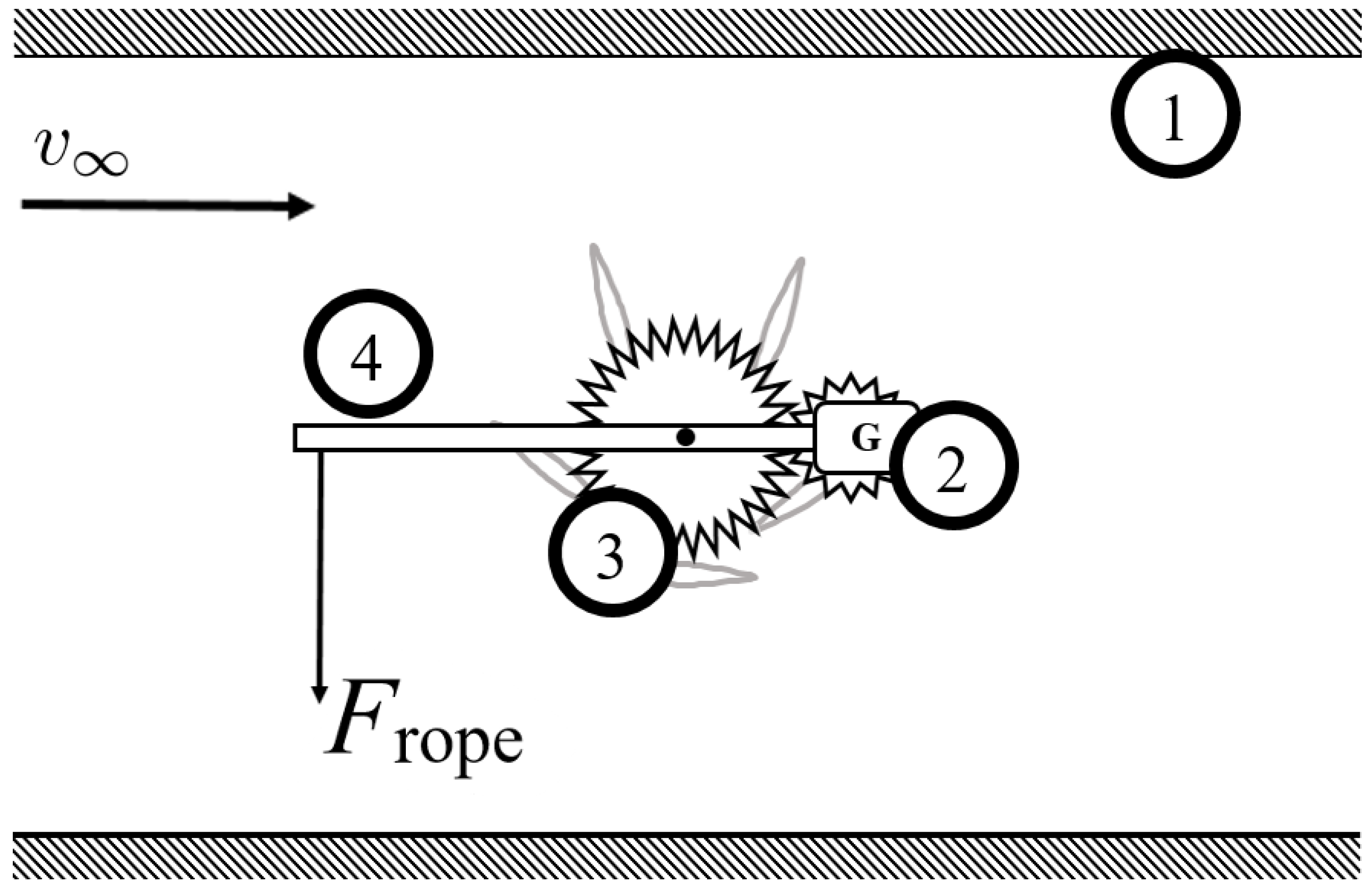
Figure 3.
Functional sketch of the measuring setup: (1) duct wall; (2) generator with pinion; (3) turbine with main gear; and (4) free-floating rod.
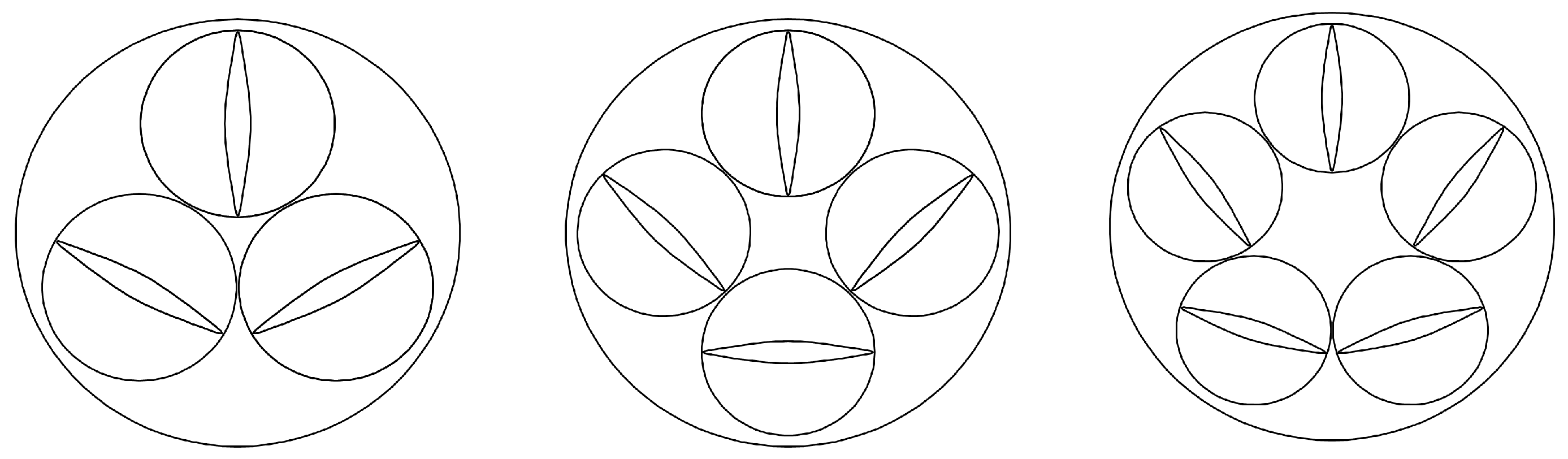
Figure 3.
Functional sketch of the measuring setup: (1) duct wall; (2) generator with pinion; (3) turbine with main gear; and (4) free-floating rod.
Figure 4.
Blade profile of the first prototype [
5].
Figure 4.
Blade profile of the first prototype [
5].
Figure 5.
Mesh convergence study for the channel flow.
Figure 5.
Mesh convergence study for the channel flow.
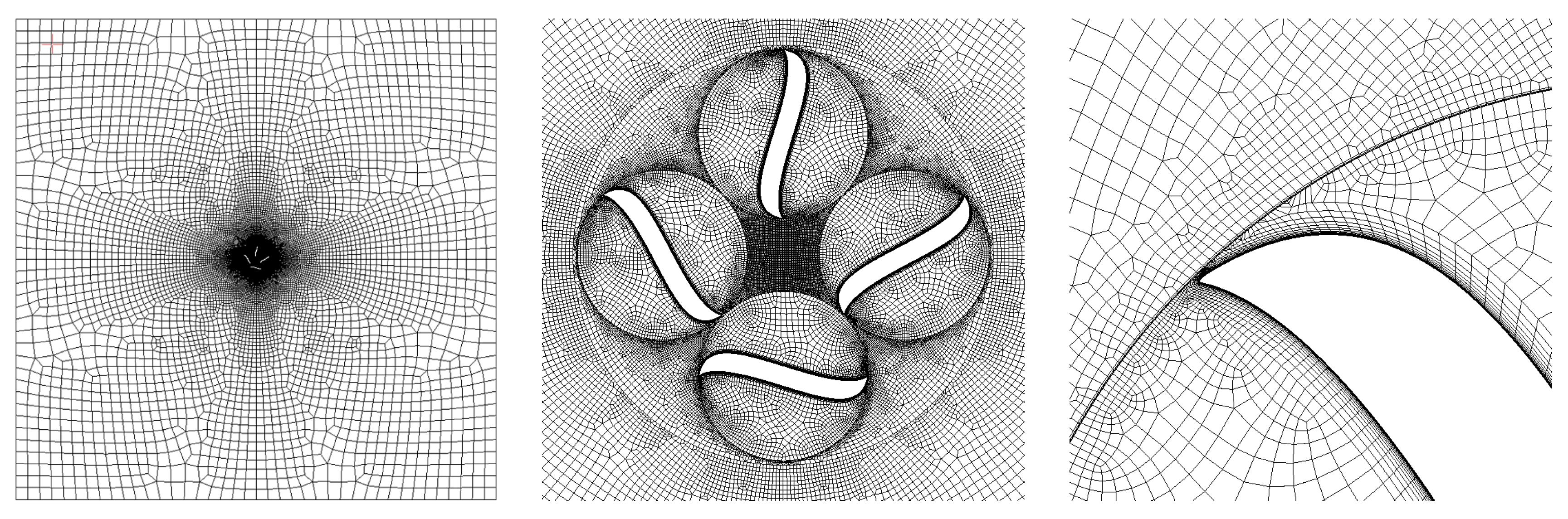
Figure 6.
Isometric view of the fluid domain with cross section through the meshing structure.
Figure 6.
Isometric view of the fluid domain with cross section through the meshing structure.
Figure 7.
Measured velocity field in front of the wheel extrapolated from 5 × 5 support points.
Figure 7.
Measured velocity field in front of the wheel extrapolated from 5 × 5 support points.
Figure 8.
Qualitative flow velocity visualization on free surface plot.
Figure 8.
Qualitative flow velocity visualization on free surface plot.
Figure 9.
Comparison of performance between simulation and experiment depending on the tip speed ratio. The error bars represent the standard deviation.
Figure 9.
Comparison of performance between simulation and experiment depending on the tip speed ratio. The error bars represent the standard deviation.
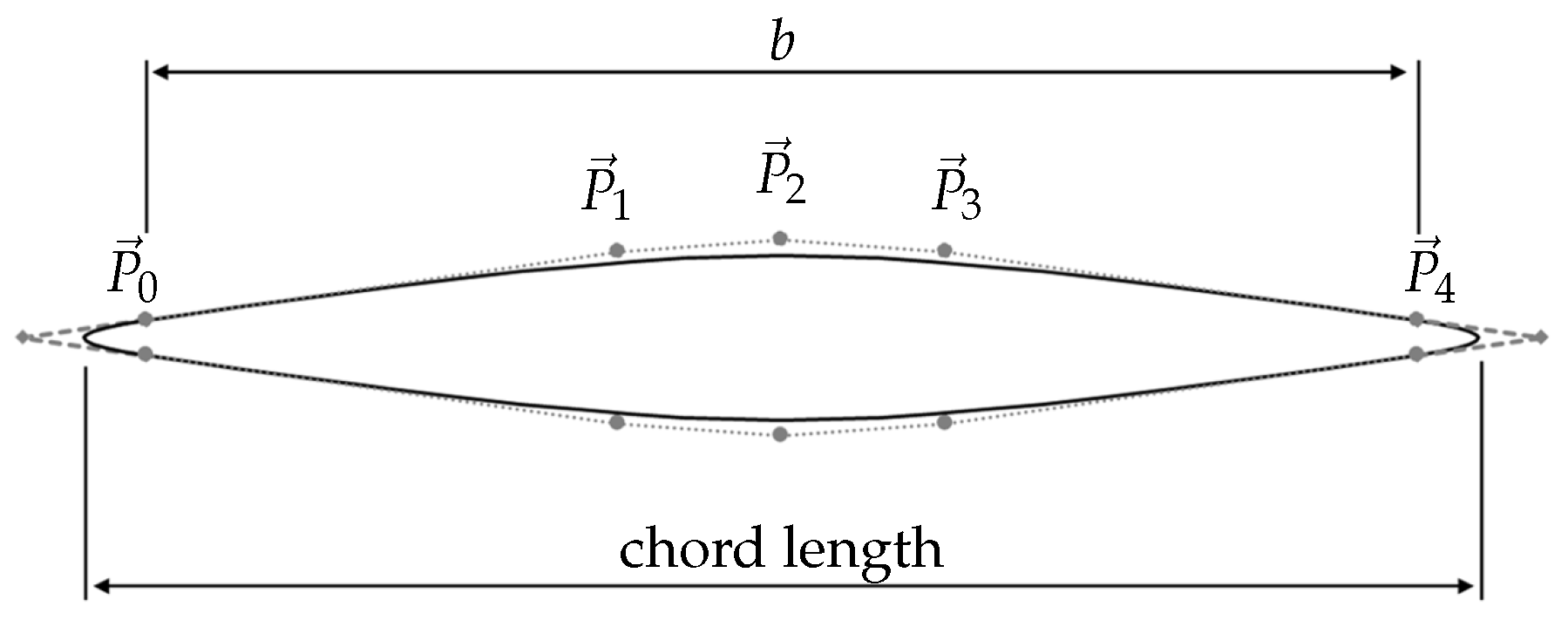
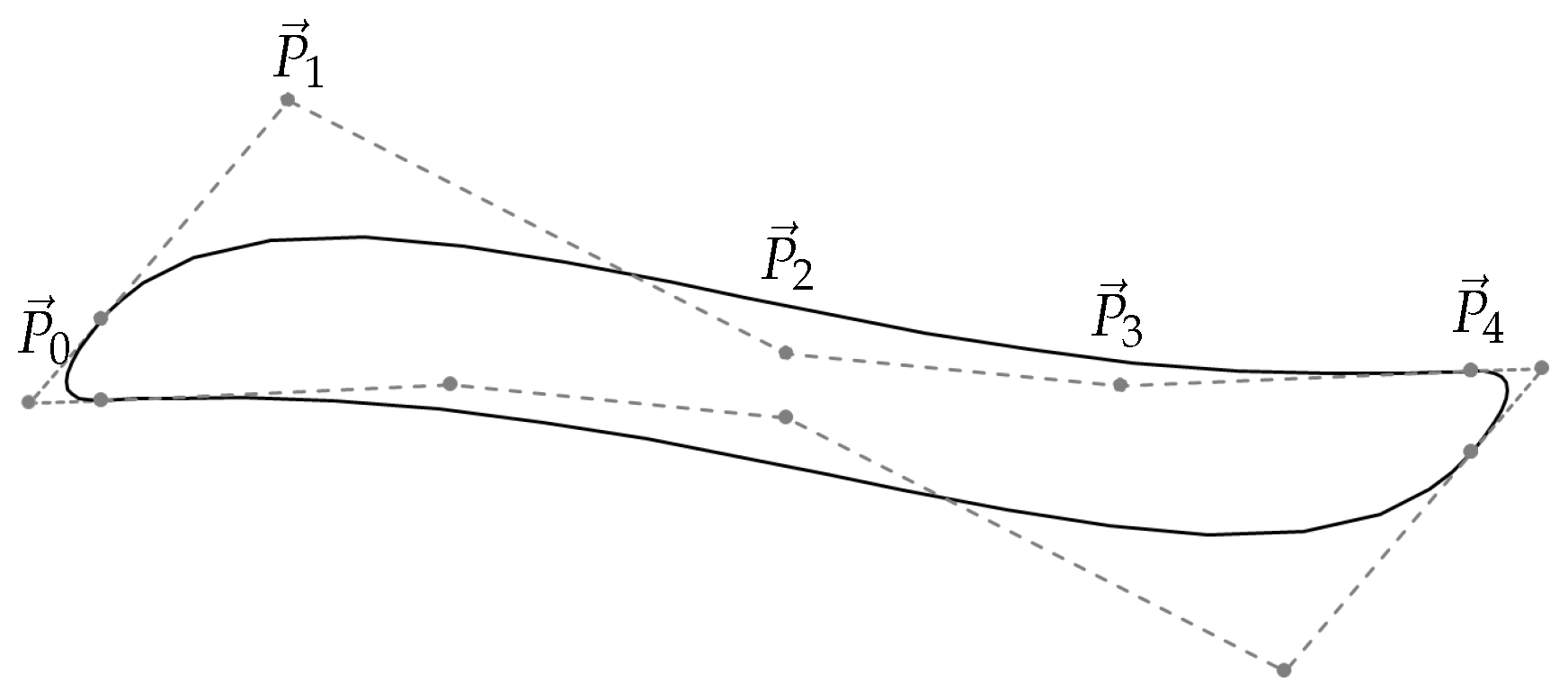
Figure 10.
Parameterized blade with Bézierspline control points.
Figure 10.
Parameterized blade with Bézierspline control points.
Figure 11.
MS Excel geometry representation with interface walls.
Figure 11.
MS Excel geometry representation with interface walls.
Figure 12.
Different number of blades with the same outer diameter.
Figure 12.
Different number of blades with the same outer diameter.
Figure 13.
Three, four and five blades compared at different phase angles. Additionally, the simulation was carried out once again in the 3D configuration at .
Figure 13.
Three, four and five blades compared at different phase angles. Additionally, the simulation was carried out once again in the 3D configuration at .
Figure 14.
Exemplary torque curve for five blades at and .
Figure 14.
Exemplary torque curve for five blades at and .
Figure 15.
Force distribution on the standard blade (No. 4) (left) compared to the best variant (No. 1) (right).
Figure 15.
Force distribution on the standard blade (No. 4) (left) compared to the best variant (No. 1) (right).
Figure 16.
Blade width factors 1 (left), 0.85 (middle) and 0.7 (right).
Figure 16.
Blade width factors 1 (left), 0.85 (middle) and 0.7 (right).
Figure 17.
Characteristic curves for different blade widths.
Figure 17.
Characteristic curves for different blade widths.
Figure 18.
Optimization process.
Figure 18.
Optimization process.
Figure 19.
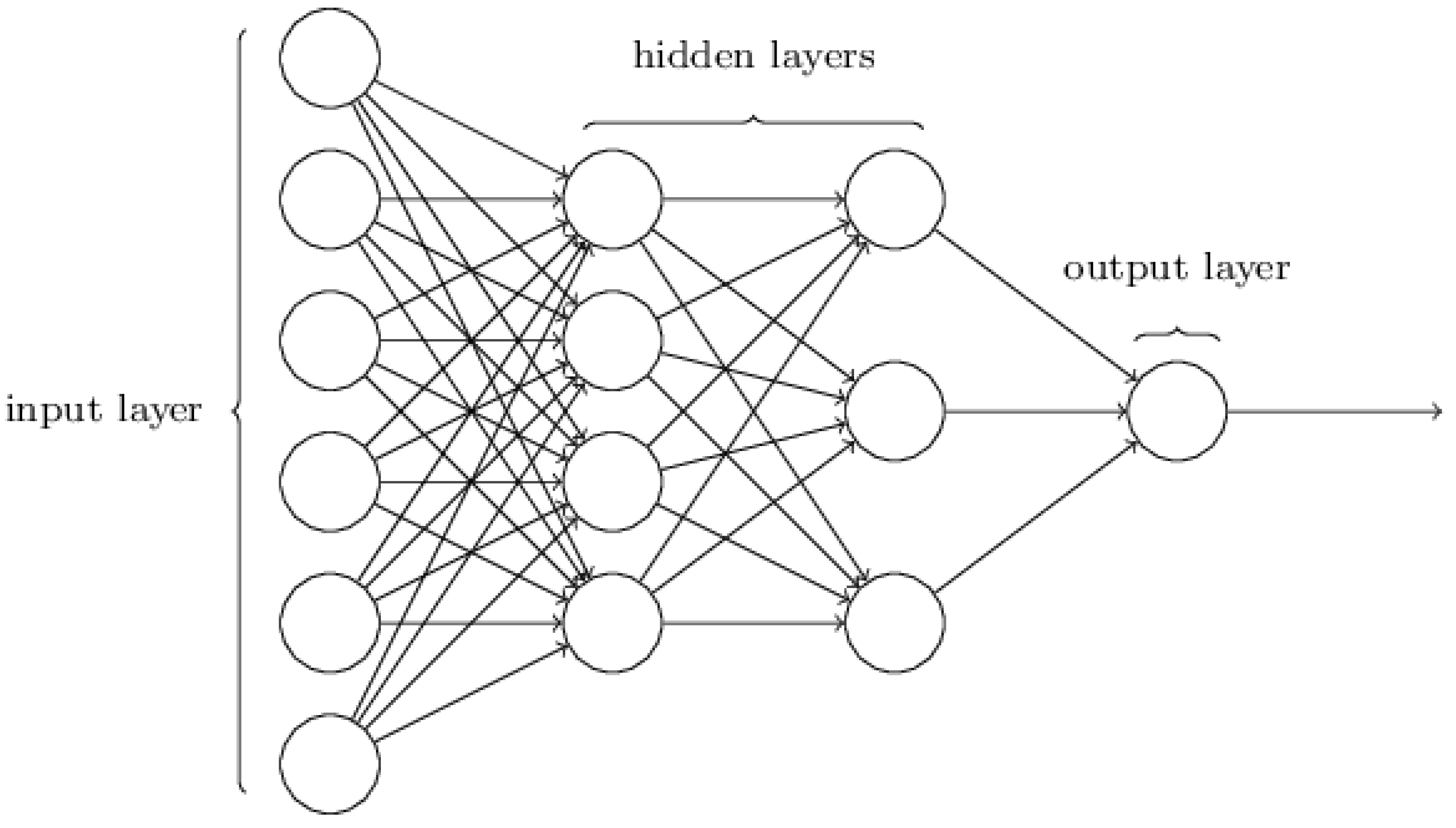
Possible network topology of an MLP [
10].
Figure 19.
Possible network topology of an MLP [
10].
Figure 20.
Point symmetrical blade.
Figure 20.
Point symmetrical blade.
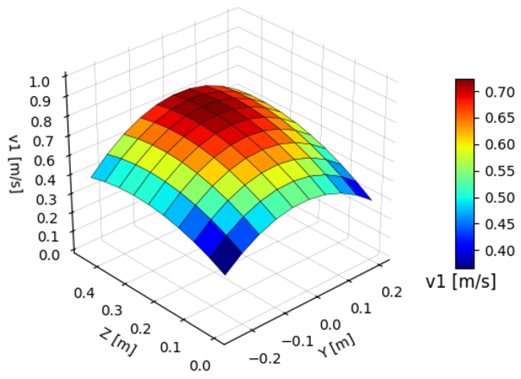
Figure 21.
Representation of parameters and with response surface.
Figure 21.
Representation of parameters and with response surface.
Figure 22.
Solutions of individual particles per time step.
Figure 22.
Solutions of individual particles per time step.
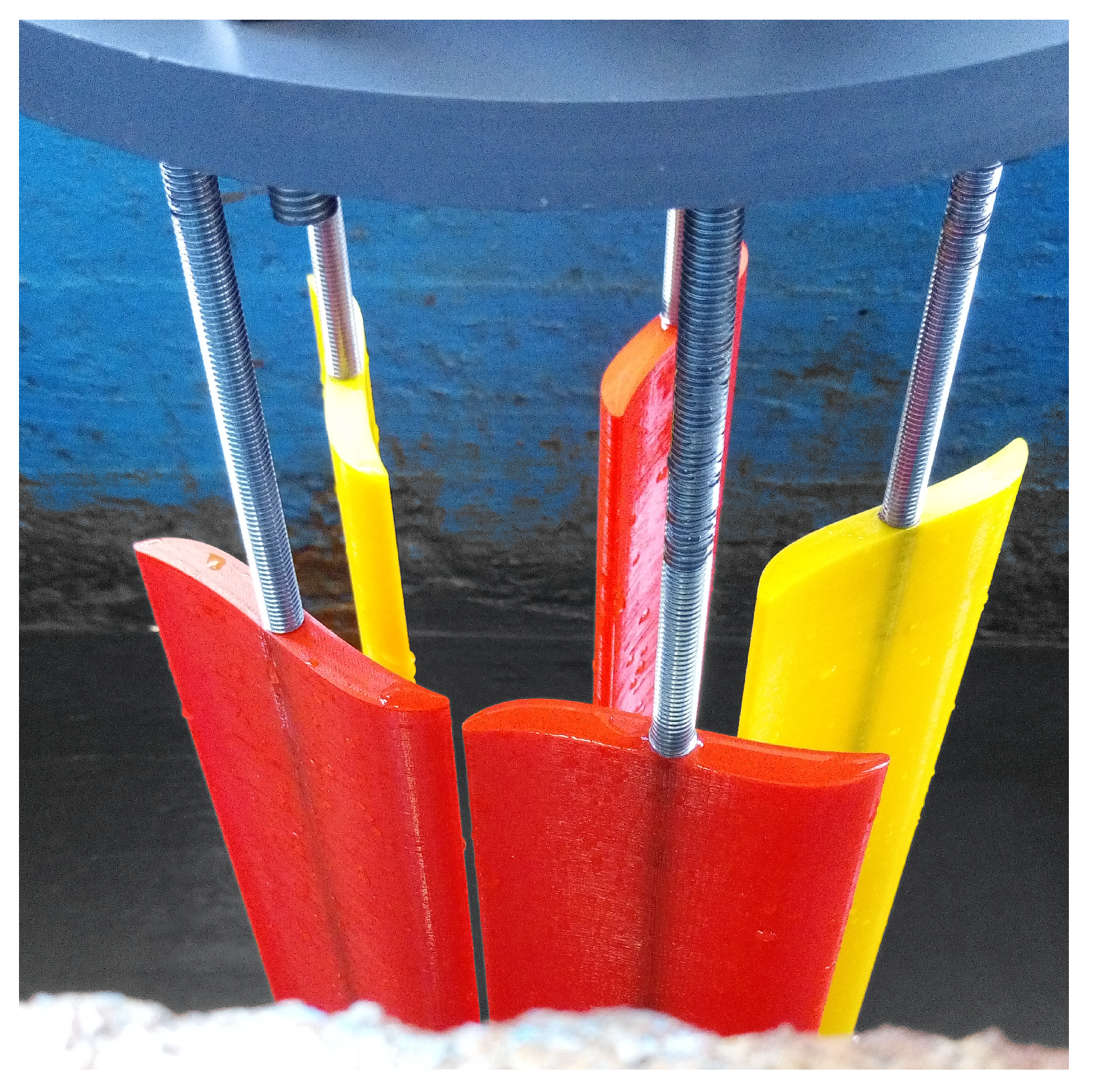
Figure 23.
3D printed blades installed on the prototype.
Figure 23.
3D printed blades installed on the prototype.
Figure 24.
Characteristic curve determined experimentally in the channel at the optimum phase angle of 10.
Figure 24.
Characteristic curve determined experimentally in the channel at the optimum phase angle of 10.
Figure 25.
Visualization of the first eight samples.
Figure 25.
Visualization of the first eight samples.
Figure 26.
Global domain (left), mesh refinement on the interfaces (middle) and inflation layer on a blade tip (right).
Figure 26.
Global domain (left), mesh refinement on the interfaces (middle) and inflation layer on a blade tip (right).
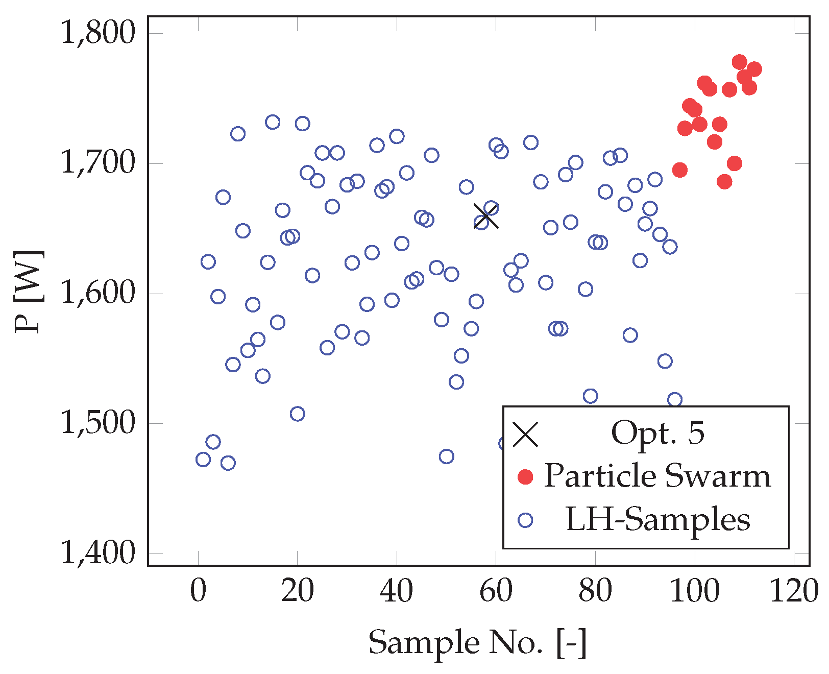
Figure 27.
Scatter plot of the power achieved for all samples and the designs generated by the PSA.
Figure 27.
Scatter plot of the power achieved for all samples and the designs generated by the PSA.
Figure 28.
PSA finds a maximum on the response surface visualized in two dimensions.
Figure 28.
PSA finds a maximum on the response surface visualized in two dimensions.
Figure 29.
Final blade design compared to the old optimum (dashed).
Figure 29.
Final blade design compared to the old optimum (dashed).
Figure 30.
Qualitative torque distribution around the circumference. The optimized blade profile leads to an increased torque generation windward while keeping the losses leeward roughly the same.
Figure 30.
Qualitative torque distribution around the circumference. The optimized blade profile leads to an increased torque generation windward while keeping the losses leeward roughly the same.
Table 1.
Definition of the control points of the upper main spline .
Table 1.
Definition of the control points of the upper main spline .
| i | 0 | 1 | 2 | 3 | 4 |
|---|
| | free | 0 | free | |
| free | free | free | free | free |
Table 2.
Definition of the control points of the left short spline .
Table 2.
Definition of the control points of the left short spline .
| i | 0 | 1 | 2 |
|---|
| | × | |
| | × | |
Table 3.
Performance comparison of different blade profiles.
Table 4.
Airfoils in comparison from the 2D simulation: Original (1); best sampling (2); and final optimization (3).
Table 5.
Airfoils in comparison in the simulated laboratory channel with free water surface: Original (1); and final optimization (2).
Table 5.
Airfoils in comparison in the simulated laboratory channel with free water surface: Original (1); and final optimization (2).
| No. | Profile | max Power [W] | Relative to Reference |
|---|
| 1 | ![Energies 12 01777 i011]() | 10.22 | 1.00 |
| 2 | ![Energies 12 01777 i012]() | 13.59 | 1.33 |


