1. Introduction
1.1. Motivation
In recent years, a microgrid-based family energy framework has increasingly attracted attention. This emerging residential energy system contains distributed Renewable Generations (RGs), household load appliances, and Energy Storage Units (ESUs). The application of residential microgrid reduces the user’s dependence on the main grid and improves the autonomy and flexibility of the family power system [
1]. In the practical field, resident users, RGs and ESUs constitute a small and independent microgrid market [
2,
3]. It’s essential to formulate an intelligent and effective residential Microgrid Energy Scheduling (MES) mechanism for coordinating and balancing the benefits of all members, meanwhile, guaranteeing the members’ self-decision ability and information security.
Besides, Electric Vehicles (EVs) are becoming more and more widespread in resident life due to its various advantages. EVs can effectively solve the pollution problem from traditional energy; in addition, the energy consumption cost of EVs is cheaper than gasoline vehicles [
4,
5]. Moreover, Vehicle-to-Grid (V2G) mode allows EVs to discharge energy to the power grid for participating in market scheduling and earning profit [
6,
7].
Considering the integration of EVs and RGs, residential MES becomes more complicated due to high uncertainties from EVs and RGs, such as RGs output and EVs’ usage attributes [
8,
9]. Therefore, some challenges exist in residential MES for previous studies shown in
Section 1.2. First, it’s difficult to build a precise scheduling model that can attend to all the uncertain parameters. Second, the common centralized dispatch methods need a completely open market environment and could be problematic with a large system and multiple constraints. Third, most works are myopic solutions considering the current objectives, instead of a long-term optimization.
As a solution to confront these challenges, a model-free machine learning method, Reinforcement Learning (RL) has got a good effect on complicated decision-making problems. However, most RL methods adopt Single-Agent RL (SARL) to obtain the optimal policy, some defects exist in SARL whether the algorithm mode is centralized or decentralized. In centralized SARL, first, microgrid control center gathers all participants’ information and implements RL tasks centrally, each participant passively performs learning results from control center, rather than learning autonomously; second, participants need to upload necessary information to control center, thus part of private information may be at risk of leaking; third, the penetration of EVs and RGs will increase computational complexity of SARL, even lead to the curse of dimensionality. On the other hand, in decentralized SARL, each participant can learn and make decisions according to individual information and environment, but SARL is a kind of selfish learning to maximize self-reward, instead of considering overall profit and supply-demand balance of microgrid [
10]; besides, the learning process of each participant is based on itself’s available information, they can’t obtain other agents’ some confidential information such as providers’ quotes and demand response behaviors of users, therefore, the agents’ learning processes are imprecise and there are no interactions among agents.
To address all the above issues, this paper presents a Multi-Agent RL (MARL) approach for residential MES. MARL is a distributed RL in multi-agent environment that can be seemed as a combine of RL and game theory [
11]. Although the MARL framework is applicable to residential MES to construct a distributed microgrid RL architecture, some limitations restrict the application of existing MARL methods in the microgrid field. First, most MARL algorithms require agents to replicate other agents’ value functions and to calculate the equilibria for all joint-actions, which are computationally expensive. Then, if agents’ information is not be fully shared (incomplete information game), it’s difficult to obtain a definite equilibrium solution [
12]. Finally, the solved equilibrium solutions may not be unique, how to select the optimal equilibrium to balance all agents’ rewards and to ensure the convergence of MARL are noteworthy [
11,
13]. In this paper, we present an Equilibrium Selection-based MARL (ES-MARL) method, an optimal Equilibrium Selection (ES) is adopted according to two mechanisms, that is private negotiation with each agent and maximum average benefit method.
1.2. Related Works
Several studies about residential MES considering EVs or RGs have been published using various approaches [
14,
15,
16,
17,
18,
19,
20]. For example, a virtual power plant based on linear programming was used as a combination of wind generators and EVs to schedule the market in [
14]. In [
15], a dynamic programming-based economic dispatch for community microgrid is formulated. The authors in [
16] proposed a hierarchical control method to achieve coordination scheduling integrating EVs and wind power. In [
17], an EV coordination management algorithm was presented to minimize the load variance and to enhance the distribution network’s efficiency. A game theory-based retail microgrid market was built and a Nikaido-Isoda Relaxation approach was adopted to get the optimal solution [
18]. A hierarchical control framework for microgrid energy management system with RGs and an ESU is proposed [
19]. Ref. [
20] studies about a day-ahead scheduling of integrated home-type microgrid and adopts a mixed-integer linear programming algorithm to achieve optimal energy management.
These previous studies cannot take all challenges in MES into account. Therefore, RL-based method is adopted as solution. RL approach learns the optimal policies through trial-and-error mechanism, that does not depend on the prior knowledge of system model information, and RL has been widely used in energy scheduling of smart grid and EVs [
12,
21,
22,
23]. For instance, ref. [
12] focused on the smart grid market based on double auction, an adaptive RL was used to find the Nash Equilibrium (NE) of energy trading game with incomplete information. The authors in [
21] proposed an RL-based dynamic pricing and energy consumption scheduling algorithm for the microgrid system. In [
22], a batch RL approach was adopted in residential demand response to make a day-ahead consumption plan. In [
23], authors raised RL-based real-time power management to solve the power allocation for hybrid energy storage system in a plug-in hybrid EV.
Moreover, in this paper, a MARL method is used for sequential decision making in multi-agent environment where traditional SARL is difficult to deal with. MARL has been adopted in some fields, such as vehicle routing problem [
24] and thermostatically loads modeling [
25]. The most universal MARL is equilibrium-based MARL, whose framework accords with Markov games and the evaluation of the learning process is based on all agents’ joint behaviors, the equilibrium concept from game theory is introduced to denote optimal joint action [
26,
27,
28,
29,
30]. The earliest proposed equilibrium-based MARL was the Minimax-Q algorithm which considered two agents’ zero-sum game, two agents try to maximize and minimize one reward function [
26]. Authors in [
27] proposed Nash-Q algorithm for non-cooperative general-sum Markov games, and the NE solution was adopted to define value function. In [
28], a friend-or-foe Q-learning algorithm was presented for obtaining different solutions based on agents’ relationships. In [
29], Correlated-Q learning was proposed base on correlated equilibrium solution, which allows for the possibility of dependencies in the agents’ optimization. In [
30], authors introduced a “Win or Learn Fast” (WoLF) mechanism to form a variable learning rate based MARL method.
These papers have made contributions on the domain of microgrid energy scheduling or RL algorithm. Through the analysis and improvement of these studies, in this paper, a MARL approach is adopted for management and decision of distributed microgrid market.
1.3. Contributions
To sum up, the principal contributions of this paper are summarized as follows.
A framework for residential MES with V2G system is built. All participants in the microgrid and the auction-based microgrid market mechanism are modeled.
MARL algorithm is introduced for the first time into a residential microgrid. The RL model (states, actions, and immediate reward) of each agent is formulated.
An improved ES-MARL is proposed, the Equilibrium Selection Agent (ESA) calculates the corresponding equilibrium solution by negotiating with agents and selects the optimal solution based on maximum average reward.
1.4. Organization
The structure of this paper is as follows. In
Section 2, we present the microgrid model and market mechanism. In
Section 3, we summarize the MARL theory and the microgrid agents’ design of MARL. In
Section 4, we propose the ES-based MARL method.
Section 5 presents the simulation results and analyses. We conclude the paper in
Section 6.
2. System Model
2.1. Residential Microgrid Description
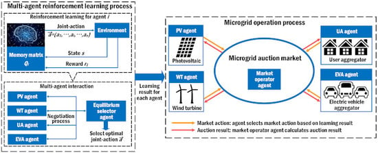
With the development of RGs and EVs, the residential microgrid has been increasingly used. For a urban residential area, the fluctuations of daily load curves are high and the distributions of residents, RGs and EVs connecting are stochastic; moreover, participants have higher requests for autonomy energy management from the perspective of economy and privacy protection; besides, residential microgrid should consider more about environmental concerts and power safety. In this paper, a distributed framework for residential microgrid which is more applicative to meet above requirements is adopted. As depicted in
Figure 1, the 9-node residential microgrid is built based on multi-agent system [
31,
32], all participants are modeled as profit-aware intelligent agents with abilities of autonomous learning and decision-making; agents in the market should comply with microgrid market mechanism and follow market scheduling based on global optimization goal.
Based on the roles in the market, microgrid agents are divided into different clusters: RGs are independent supplier agents; users are consumer agents and can join in microgrid scheduling through demand response; a unified management for EVs acts as supplier agents or consumer agents according to overall charging/discharging action; besides, manager agents (e.g., market operator and equilibrium selector) are set to maintain market operation. The primary objective for the microgrid in grid-connected mode is to achieve maximum autonomy, that is to provide the necessary load demand with the minimum dependency on Utility Grid (UG). Besides, agents’ benefits should be considered to realize a unanimously acceptable balance. All agents’ concrete models are described as follows.
2.2. Microgrid Components
2.2.1. Electric Vehicles
EVs are both power consumers and power suppliers in the microgrid market. Considering the negative effects of V2G, extra battery degradation cost and the impact on subsequent travel should be considered to evaluate the net profit of V2G. Distinct from stationary ESUs, EVs’ charging/discharging actions will be affected by owners’ traveling habits and stochastic behaviors of EVs usage. Besides, specific operational and technical constraints of EVs should be noticed.
(1) EV Travel Behaviors and Constraints: EVs charging/discharging scheduling should take travel demand as premise. The customary travel habits (e.g., arrival time, departure time and travel distance) follow a similar pattern based on the owner’s intentions, besides, the random characters of travel behaviors are considerable [
33].
The State-Of-Charge (SOC) of EV
i at slot
t is defined as
,
is the current number of EVs,
. The constraints of EVs SOC is:
where
and
are minimum and maximum limits of EV battery SOC, respectively. The charging/discharging limitations are:
where
is EV
i’ charging/discharging power at slot
t,
is positive when EV is charging and is negative when EV is discharging.
and
, where
and
are EV
i’ battery charging and discharging rate. Then, we have:
where
is EV
i’ battery capacity. If EV
i will leave at slot
t, SOC should satisfy the travel demand as:
where
is EV
i’ minimum SOC for departure. Remarkably, only if EVs adopting slow-charge can participate in the microgrid market; if EVs need urgent travel, the fast-charge will be chosen. The EV owner’s travel habits are from data statistics, arrival time and departure time follow normal distribution; and travel distance follows a log-normal distributed.
(2) EV Battery Degradation Cost: The life of EV battery declines along with repeating charging/discharging cycles. For lithium iron phosphate battery adopted in this paper, low temperature weaken performance and high temperature curtails battery life. The use of battery in moist condition should be avoided. Besides, a prolonged period of overvoltage during long travel may stress the battery [
34]. In sum, we consider that EVs battery degradation depends on the number of cycles. According to [
35], the battery degradation cost function can be approximately expressed as:
where
is battery degradation cost of
,
represents battery cost,
k is the slope of the linear approximation of the battery life as a function of the cycles.
(3) EV Aggregator and EV Secondary Scheduling: In our model, an EV Aggregator (EVA) is adopted to manage all EVs’ participation in the market. The introduction of EVA facilitates the model extendibility and adjustment when the number of EVs changes, besides, the reduction of agents number can improve the convergence speed of learning algorithm.
Base on [
33], all local EVs participating in the microgrid market (primary market) form a secondary scheduling system of EVs, EVA is the manager of the secondary scheduling system. At the beginning of each slot, EVA arranges each EV’s charging/discharging amount based on the optimal global charging/discharging action from the primary market, besides, some rules should be obeyed as follows.
EVs’ travel demand should be satisfied, first of all, EVA considers EVs’ travel demand two hours ahead of departure and guarantees SOC is more than .
EVA arranges EVs charging/discharging sequence according to SOC level, if , this EV can’t discharge and should be arranged to charge, where is charge warning limit.
The total charge/discharge amount from the primary market is the scheduling objective of the secondary system, the sum of EVs’ charge/discharge should be equal to the total amount.
2.2.2. Users’ Loads
The residential appliances keep approximately steady in identical period during the same season, therefore, users’ load demand can be predicted accurately. User
i’s load demand at slot
t is written as
,
,
and
are minimal essential demand and maximal available demand, respectively.
is the number of users,
. According to operating profiles, the household load can be categorized into three types as follows [
36].
(1) fixed loads: this kind of load demand can’t be changed to guarantee the devices in working order, such as web servers and medical instruments. User i’ critical loads profile is denoted as .
(2) curtailable loads: the demand can be cut down for reducing consumption, such as heating or cooling devices.
denotes the load profile of curtailable loads, and we denote the
as the ratio of load curtailment. Then, we have:
where
is the fixed part of curtailable loads, if
, this kind of devices becomes fixed loads; if
, user can turn off these devices.
(3) shiftable loads: the operation period can be postponed to avoid the load peak, such as the washing machine. The shiftable loads profile is , if user postpones the loads demand , the shiftable part will defer to the next time slot for consideration.
In sum, user
i’ total load demand
. Therefore, after demand response, user
i’ actual load demand can be denoted as:
Users can regulate the schedules of curtailable loads and shiftable loads to control the load consumption; meanwhile, load curtailment and shift will reduce the user’s consumption satisfaction. In this paper, a utility function
which represents user’s satisfaction is adopted as:
where
indicates users’ action (a larger
implies a larger utility);
denotes the utility saturation. The utility function should be non-decreasing and concave. Similarly, in the learning process of MARL, a User Aggregator (UA) is introduced to centrally arrange the demand responses of all users.
2.2.3. Renewable Generations
RGs’ generation capacity can be derived from accurate short-term forecasts via historical data and environmental data. The random characteristics of RGs’ generation are represented as stochastic normal distribution based on forecast results.
From [
37], the generation of PV
is closely affected by the weather factors,
is determined as:
where
is conversion rate of PV array (%);
is area of PV array (
);
is solar irradiance which is from the Beta probability density function (
) [
1];
T is the average temperature during
t (
).
The main element influencing the output of WT is wind speed
. The WT generation
is a piecewise function of
denote as below [
38]:
where
and
are the cut-in wind speed and cut-off wind speed, respectively;
is the rated wind speed;
is the rated power of WT.
2.3. Transaction with Utility Grid
Microgrid keeps supply-demand balance through energy trade with UG, the transaction prices between UG and microgrid are fixed by UG. Here, UG adopts a real-time price mode that the price is variable at each time slot. The trade price between UG and microgrid market is summarized as a tuple
,
is purchase price from UG, and
is sell price to UG. To avoid energy arbitrage,
is perpetually lesser than
, a factor
is defined as sell/purchase price ratio [
39].
2.4. Microgrid Market
As suggested by [
33,
40], a real-time microgrid market is constructed based on a one-side dynamic bidding model. In the microgrid market, supplier agents provide their quotes with bid price and supply amount; consumer agents submit their energy demand which can be optimized by adjusting their consumption behaviors. The above information of sellers and consumers aggregate in a non-profit Market Operator Agent (MOA), whose duty is to make the market clearing price
and to calculate each agent’s energy sell/purchase amount. The microgrid market operates per time slot
t, abiding the following principles.
In the market clearing process, MOA sorts sellers’ quotes in increasing order of prices, then the demand will be matched according to the ranking and respective supply. The bid price of the last adopted quote is defined as the marginal price, that is the market clearing price .
If the energy supply is lacking to support the load demand, MOA will purchase energy from UG. The purchase price from UG is higher than the sellers’ bids. The additional expenditure will be charged averagely by all purchasers.
If the supply exceeds the demand, the surplus energy will be sold to UG. If more than one seller offers the market clearing price, their energy sold to microgrid and UG are arranged based on the same proportion of their supply.
3. MARL Method for Microgrid Market
For a multi-agent based microgrid system, the most important task is to generate agents’ distributed strategies to schedule their behaviors in the market. Moreover, it’s significant to ensure all agents’ benefits balance. In this section, a MARL method is introduced to solve this issue about how to generate and coordinate the autonomous strategies for all agents.
3.1. Overview of MARL
RL algorithm is an unsupervised machine learning method for sequential decision problems. In SARL, agents interact with the environment by executing actions, the environment then feeds back an immediate reward to evaluate the selected action. Transfer to MARL, the relationships with both cooperations and competitions exist among agents, and agents’ rewards are influenced by other agents’ states and actions. SARL is built on the framework of Markov Decision Process (MDP), but in MARL, the framework is Markov game, which is the combination of MDP and game theory [
41,
42].
Definition 1. Markov Game. An n-agent () Markov game is a tuple , where n is the number of autonomous agents; S is the state space of system and environment; is the action space of agent i, , then the joint-action space is defined as and a joint-action ; is the immediate reward function of agent i; P is the transition function, denotes the probability distribution when an action is executed, the current state transfers to a new state, .
As shown in
Figure 2, compared with SARL, the main distinction of MARL is that the reward function and state transition for agents are based on the joint-action
. In a pure strategy game, the agents’ joint-action is defined as
, in MARL, when
is applied and the state transfers from
s to
, an action evaluation Q-function for agent
i,
is defined as:
where
is the maximum discounted cumulative future reward starting from state
;
is the discount factor, which indicates the weight of future reward.
In SARL, agent
i’s goal is to find an optimal action policy
to maximize Q-function, but the goal in MARL is to find an optimal joint-action
to coordinate all the Q-functions
to a global equilibrium. A concept of equilibrium solution from game theory is introduced into MARL. The generally used equilibrium solution is NE [
27].
Definition 2. Nash Equilibrium. In a pure strategy Markov game, a NE solution is defined as a joint-action , satisfying the following criterion for all n-agents: An intuitive comprehension about NE is that, for all agents, if other agents don’t change their actions
, agent
i can’t improve its utility function
by changing itself’s action
, where
is the joint-action of all agents except agent
i. At time slot
t, the iterative modified formula of Nash-Q MARL is expressed as:
where
is the learning rate, whose value decides convergence speed of MARL.
is agent
i’ Q-value with the selected NE in the next state
.
In general, the major structures of other equilibrium-based MARL algorithms are similar to Nash-Q MARL, the main difference is various selected equilibrium in the learning process.
3.2. Agents Design for Microgrid MARL
The equilibrium-based MARL is applicable in a mixed task (competitions coexist with cooperations) multi-agent system, in the residential microgrid market, there are both competitive relations (e.g., suppliers’ quotes) and cooperative relations (e.g., sellers and purchasers collaborate to achieve supply-demand balance and microgrid autonomy). Detailed formulations of MARL used in residential MES are introduced in this section.
First of all, all agents’ MDP models are designed as follows.
3.2.1. EV Aggregator Agent
In the primary microgrid market, EVA agent participates in the market as a centralized agent of all EVs. EVA decides the total charging/discharging in the market based on MARL results. In EVA’s learning process, the current local EVs number, SOC and travel demand of EVs should be considered.
State: The state-base for EVA agent at slot
t is defined as:
where
is the average SOC of local EVs;
is the number of local EVs, which connect with microgrid. According to
t, we can get the UG price
.
Action: EVA’s actions include total charging/discharging power
and EVA’s quote
.
, EVA acts as a purchaser;
, EVA serves as a seller;
means that there is no energy trade. Only when
,
is existent. The action-base of EVA agent is denoted as:
Considering that only if the EV is connected to microgrid (non-movement state), the charge/discharge action can be executed [
43], so the action of EVA is constrained by average SOC
, local EVs’ number
and travel demand (denoted by
). The total charging/discharging power
is confined as:
Besides, when , EVA can only select energy purchase actions; when , EVA can only select energy sell actions.
Reward: According to statistics, more than 90% of EV users will charge the SOC up to 60% before leaving. The user’s anxiety due to the worry about exhausting energy on the road aggravates increasingly with the decline of SOC. Therefore, the immediate reward function of EVA should combine economy, battery degradation, and user’s anxiety, which is defined as:
where
and
are the charging/discharging anxiety coefficients.
is the average battery capacity of all EVs.
and
are the energy trade with microgrid and with UG, respectively; when
,
; when
,
.
3.2.2. User Aggregator Agent
From
Section 2.2.2, users can control curtailable loads and shiftable loads to reduce cost; meanwhile, the load adjustments depress users’ satisfaction. UA agent takes a uniform demand response action based on the results of MARL, then the demand response task is assigned averagely to all users in the secondary scheduling.
State: The state-base of UA agent at slot
t is defined as:
where
t is current time slot;
is cumulative load demand of all users without demand response.
Action: The action-base of UA agent at slot
t is defined as:
where
is the total ratio of load demand curtailment;
is the cumulative shiftable load demand. Then,
, where
,
and
are total demand of fixed load, curtailable loads and shiftable loads, respectively.
Reward: Similar to Equation (
7), the actual cumulative load demand is defined as
UA agent’s immediate reward function
is defined as the difference between users’ total utility function and energy purchase expenses.
where
,
and
are the energy purchase from microgrid market and UG, respectively.
3.2.3. RG Agents
There are two kinds of RGs, Photo-Voltaic (PV) and Wind Turbine (WT), the output of RGs is based on the short-term forecasts, and random distributions with forecast values will be adopted to embody the uncertainties of RGs’ generation. All of the RGs’ generation will be put into the market at the current time slot.
State: The state of RG agents is current time slot
t.
Action: The actions of RG agents are denoted as:
where
are the quote prices of PV agent and WT agent.
Reward: The RG agents’ immediate reward functions are profit functions as:
where for the tuple
,
is the portion sold to microgrid;
is the portion sold to UG,
.
is the generation cost function, which is considered as a quadratic function as:
where
are pre-determined parameters which are different for PV and WT, and
.
3.3. MARL Method for Residential MES
Based on agents’ MDP model designs, the equilibrium-based MARL is adopted. The general framework of agents’ learning process for microgrid MARL is shown as Algorithm 1.
At line 3 of Algorithm 1, -greedy policy denotes that the agent selects a random action with a probability of and selects a joint action which makes system achieve equilibrium with a probability of . is the expected value of the equilibrium in state .
| Algorithm 1 General Framework of Microgrid MARL |
| Input: |
| Agent set N; state space ; action space ; learning rate ; discount factor ; joint action space A.
|
- 1:
Initialize ; initialize state , and ; - 2:
repeat - 3:
For each time slot t, each agent selects with -greedy policy to form a joint-action ; - 4:
MOA calculates the market clearing price and the energy should be traded of each agent; - 5:
Each agent obtains the experience (); - 6:
Each agent updates the Q-matrix : - 7:
, ; - 8:
until Q-matrix converges.
|
| Output: |
| The optimal Q-matrix for each agent.
|
4. Improved Equilibrium-Selection-Based MARL
As mentioned in
Section 1.1, some limitations existing in common MARL algorithms, are summarized as follows.
In the learning process of common MARL, agent updates and saves other agents’ value functions in each iteration step, that will cause a huge computation work, even in a small scale environment with two or three agents.
In order to work out the equilibrium solution, MARL needs agents to share their states, actions and value functions, including some privacy information, which is unrealistic in some situations.
In each learning iteration step, there is perhaps more than one equilibrium solution, different equilibria bring different updates of value functions, which may lead to non-convergence of the algorithm. Besides, it’s hard to ensure fairness for selecting an equitable equilibrium because agents’ rewards are different with different equilibria.
Therefore, we present an ES-MARL algorithm to address these issues. We set up an Equilibrium Selection Agent (ESA), whose function is to separately negotiate with all agents to get the equilibria solution set and to select the optimal equilibrium based on the maximum average benefit method.
4.1. Negotiation for Equilibrium Solution Set
In an incomplete information game, agent’s reward information is incompletely public to other agents, agents can’t obtain other agents’ value functions to compute the equilibria. To solve this problem, according to [
11], ESA is adopted as a neutral negotiator to communicate with each agent privately to obtain their potential equilibrium set following these steps:
At the beginning of slot t, agent i finds its potential NE set and sends it to ESA (concrete steps for finding potential NE set are shown in Algorithm 2).
ESA selects the joint-action , which meets the criteria , into the final equilibrium set , the selected is the pure strategy NE solution of game .
If there is no joint-action satisfying NE, ESA selects whose number of satisfying , is the most and (more than half agents get to equilibrium), then adds into .
Now, the equilibria set is the candidate set by negotiations, the element number of may be more than one.
| Algorithm 2 Equilibrium Selection Process of MARL |
| Input: |
| Agent set N; current state ; joint-action space A; agent number n; weight factor . |
- 1:
Potential NE set ; final equilibrium set ; - 2:
for each do - 3:
; - 4:
; - 5:
end for - 6:
Each agent sends its to ESA; - 7:
; - 8:
for each do - 9:
ifthen - 10:
; - 11:
else - 12:
Calculate , which is the number of ; - 13:
end if - 14:
if then - 15:
is the final pure strategy NE set; - 16:
else - 17:
if then - 18:
; - 19:
, is the final suboptimal set; - 20:
else - 21:
; - 22:
end if - 23:
end if - 24:
end for - 25:
for each do - 26:
Calculate the value of joint benefit function: ; - 27:
end for - 28:
;
|
| Output: |
| The optimal equilibrium .
|
4.2. Equilibrium Selection Based on Maximum Average Reward
If the element number of
is more than one, the update of Q-function shown as Equation (
13) will get different values based on different selected equilibria. In this paper, a maximum average reward method is adopted to help ESA selecting the optimal equilibrium to guarantee algorithmic efficiency and fairness.
Here, we introduce an average reward function
J which denotes all agents’ average reward as:
ESA selects the optimal equilibrium (joint action ), whose corresponding value of J is maximum. The selected optimal equilibrium is used in MARL to update Q-functions. The ES process is shown in Algorithm 2.
Based on the optimal equilibrium joint-action , an improved ES-MARL algorithm is shown in Algorithm 3. Private negotiations between ESA and other agents can avoid redundant updates of Q-functions for each agent and protect the privacy information; meanwhile, the optimal ES process can combine all agents’ benefit and promote global welfare. The fairness, safety, and efficiency of the microgrid market are guaranteed with ES-MARL.
| Algorithm 3 ES-Based MARL Algorithm |
| Input: |
| Agent set N; state space ; action space ; learning rate ; discount factor ; joint action space A.
|
- 1:
Initialize ; initialize state , and ; - 2:
repeat - 3:
For each time slot t, agents select random with probability or adopt an optimal equilibrium joint-action based on Algorithm 2 with probability ; - 4:
MOA calculates the market clearing price and the energy should be traded of each agent; - 5:
Each agent obtains the experience (); - 6:
ESA computes the optimal equilibrium of next slot based on Algorithm 2; - 7:
Each agent updates (with -greedy policy): - 8:
, ; - 9:
until Q-matrix converges.
|
| Output: |
| The optimal Q-matrix for each agent.
|
4.3. Overall Process of Proposed ES-MARL Approach
To sum up, we present a flowchart shown in
Figure 3 about proposed ES-MARL approach for microgrid energy scheduling, including the MARL training process and MARL application process. From
Figure 3, we can see in the training process of ES-MARL algorithm, the ES procedure (shown in
Section 4, Algorithm 3) is responsible to connect all agents and select optimal joint-action for agents; then the learning process (show in
Section 3) is based on agents’ MDP models and microgrid model to perform the Q-function iteration of each agent; the learning result is each agent’s optimal Q-function. Adopting the learning results into practical microgrid market operation (the market model is shown in
Section 2), each agent selects current optimal action to participate in the market based on respective current state information and the optimal Q-function.
5. Simulation Results and Analysis
In this section, three parts of simulations are conducted to evaluate the proposed MARL algorithm for residential MES. First, the performances of MARL and SARL for MES are compared; then, the effect of proposed ES-MARL is verified and Nash-Q algorithm is used as comparison; finally, the secondary scheduling system of EVs is simulated.
In our microgrid model, an urban residential district is considered. The RGs in the microgrid include one PV and one WT. RGs’ daily forecast outputs are extracted from the historical data of a certain area. In microgrid market operation simulations, stochastic models of RGs’ generation are used, RGs’ actual generation values are generated from probability distributions based on the forecast outputs, the probability distributions of PV and WT are based on [
44]; the generation cost functions for PV and WT are
and
.
Figure 4a shows the real-time energy purchase price from UG; fiducial forecast values of PV output, WT output; and users’ total daily load demand. The number of users is 3; user utility function is
, where the interval of
is
, and the value of
is high or low correspond to load peak period or load trough period, and
.
In our microgrid, there are 10 EVs, EVs’ parameters are shown in
Table 1. Besides, from [
45], the number of arriving EVs or departing EVs at slot
t follows normal distribution
and
,
and
are standard values shown as
Figure 4b. EVs battery SOC bound is between 0.2 and 0.9; the SOC of arrivals is sampled from
; the travel distance of EV
D follow a log-normal distribution
. All simulations are conducted using Matlab 2018a on the personal computer with Inter Core i7-6700 CPU @3.40GHz.
-greedy strategy is adopted in MARL for action selection strategy,
; other learning parameters in RL are shown in
Table 2.
5.1. Performance Comparison of MARL and SARL
5.1.1. Each Agent’s Benefit in Different RL Methods
To verify that MARL structure is more applicable than SARL structure in the microgrid market, we simulate the operation of the adopted microgrid model based on the learning results of proposed ES-MARL and various SARL configurations. In SARL, agents can only use public information and their information to learn optimal strategies, and they estimate other agents’ privacy information according to experience knowledge. Besides, the agent’s learning objective in SARL aims to maximize individual benefit. As contrasts, five SARL configurations are used: in the former four systems, only one kind of agent has learning ability (SARL-PV only, SARL-WT only, SARL-UA only and SARL-EVA only), microgrid market operates with the optimal strategy of learning ability agent, other agents adopt fixed action based on current time slots; in the last SARL, all agents have individual learning ability (SARL-all agents), the market works with selfish optimal strategies from each agent’s SARL. We separately evaluate four agent’s daily profit in different configurations, the results of stochastic microgrid operation lasting for 30 days are shown in
Figure 5,
Figure 6,
Figure 7 and
Figure 8. In
Figure 5 and
Figure 6, daily profits of RGs
; in
Figure 7, daily welfare of UA
; in
Figure 8, daily total expense of EVA agent is the difference between total electricity purchase cost and total sale income.
From
Figure 5,
Figure 6,
Figure 7 and
Figure 8, we can see if only one agent has RL ability, the profit of this agent is always highest (or expense is lowest), agent with RL ability can make the optimal decisions based on current market state, but other agents’ fixed actions are not optimal for increasing their profit. Moreover, the effects of the proposed ES-MARL method keep in second place for all the four agents. Considering the benefit balance of all agents, it is reasonable that the result of MARL is not as good as selfish SARL for only one agent. However, the global performance of MARL for all agents is optimal. Besides, there are some other notable results. The profits for all agents in SARL-all agents case are the worst, the reason is that in this case, all agents make actions based on their selfish learning results which only care about the self-benefit, this will lead to the imbalance of market and reduce global benefits. We also can find that the curves of SARL-PV only, SARL-WT only and SARL-UA only are more stable (EVA without learning ability), a reasonable explanation is that the randomness of EVs is far more than other members, with RL learning ability, EVA performs actions with the random states of EVs, so the market scheduling results will fluctuate.
5.1.2. Overall Performance in Different Microgrid Configurations
For an MES, market fairness and microgrid independence are the two most important indicators. Fairness is to guarantee all participants’ benefits achieving equilibrium; microgrid independence aims to realize the supple-demand balance and reduce dependency on UG. Therefore, two global indexes, agents’ average profit and daily energy purchase from UG, are introduced to evaluate overall performance. Agents’ average profit indicates the overall benefit of microgrid operation; daily energy purchase from UG indicates the dependence level of microgrid on UG. Moreover, to verify the algorithm validity in general cases, two different microgrid configurations are adopted for operation with different RL methods. Microgrid configuration 1: one PV, one WT, 3 users and 10 EVs; microgrid configuration 2: 3 PV, 2 WT, 8 users and 20 EVs. The results are shown in
Figure 9,
Figure 10 and
Figure 11.
As depicted in
Figure 9, agents’ average profit is highest with ES-MARL in the two configurations, the value keeps between 30 and 40 for microgrid 1 and 50 to 70 for microgrid 2. This result indicates that ES-MARL produces the best performance to maximize global benefit comparing to other SARL methods. In addition, we can see that the average profits in SARL-PV only, SARL-WT only and SARL-UA only are almost close to zero, the reason is that the demand of EVs’ charge is higher than RGs’ supply, if EVA has no learning ability to make optimal decisions, the charging cost of EVs is expensive, therefore, the average benefit is offset by EVs’ charge expense in these three cases.
Figure 10 and
Figure 11 illustrate the microgrid has the best independence with ES-MARL, the energy purchases from UG in the two configurations are both minimal. The learning process of MARL is based on joint learning, sellers and buyers can reach to appropriate equilibrium to balance the market, agents learn from each other to decrease the supply-demand gap, the microgrid doesn’t need to buy more expensive energy from UG. The lower half of
Figure 10 and
Figure 11 (energy purchase from UG are higher in these cases) also show the importance of EVA agent’s learning ability. Combined
Figure 10 and
Figure 11, the ES-MARL method has the best performance in energy trade with UG; besides, different microgrid models don’t affect the final performance of our approach.
5.2. Performance of Improved ES-Based MARL
In this section, several simulations are conducted to evaluate our improved ES-based MARL algorithm. Here, we use Nash-Q MARL algorithm as a comparison, Nash-Q algorithm is the most commonly used MARL. The main difference between Nash-Q and proposed ES-MARL is the equilibrium selection in value function update. We study the algorithm performance from two aspects: performance in the learning process and application effect in residential MES. The RL parameters in two algorithms are set as same as
Table 2.
First, four agents’ learning performances of the iterative process are shown in
Figure 12 and
Figure 13. In
Figure 12 and
Figure 13, the label of the x-axis is episode, which denotes one state transition period from initial state to terminate state, in this paper, one episode is equal to one day (0:00–23:00). The label of the y-axis is Q-value, which is the updated value of Q-function in the current slot. From the results of four agents’ Q-values, we can see, the Q-values of ES-MARL is higher than that of Nash-Q throughout the learning process. A bigger Q-value means that the agent’s current reward is higher, so ES-MARL can gain a better strategy to increase reward than Nash-Q. Besides, from the curves’ trends of four the agents, there is a clear gap in the convergence rates between two algorithms. The state-spaces of the four agents are different (PV’s and WT’s are smallest, EVA’s is biggest), therefore, convergence speeds are accordingly different. For PV and WT, ES-MARL reaches a stable value when
, however, Nash-Q reaches a stable value when
. For UA and EVA, the convergence episode of ES-MARL is about
and
, but when
, the curve of Nash-Q trends to a stable value. The above results show that the convergence speed of ES-MARL is faster.
Then, the results shown in
Figure 14,
Figure 15,
Figure 16 and
Figure 17 illustrate the application performances of the two algorithms when their learning results are adopted in the microgrid market operation. In
Figure 14,
Figure 15 and
Figure 16, we simulate a one-day microgrid operation with ES-MARL and Nash-Q. The data points of all simulations are calculated by the average value of 100 Monte Carlo experiments.
Figure 14 shows the hourly profit of PV and WT. The profits of PV and WT with ES-MARL are superior than with Nash-Q in most hours. The total profits are higher for ES-MARL.
Figure 15 depicts the results for UA agent, including two indicators, total energy purchase expense and total welfare (difference between users’ total utility function and total expense), the results show that with ES-MARL, the expense is lower and welfare is higher for UA agent. EVs are both seller and purchaser in the market, the total charge expense and discharge profit of EVA agent are shown in
Figure 16. The performance of ES-MARL is better than Nash-Q for less expense and higher profit. To summarize the above analysis, the application performance of ES-MARL is overall better than Nash-Q for all agents. Finally, turn to energy trade between microgrid and UG, consider that energy trade is not the same in the specific hour for different days due to random parameters, we simulate microgrid operation for 30 days as shown in
Figure 17. The amount of energy purchase from UG of ES-MARL is less than that of Nash-Q, ES-MARL can reduce microgrid’s dependency on UG compared with Nash-Q. Meanwhile, the microgrid will sell back more energy to UG after adopting ES-MARL.
5.3. A Simulation Case of EVs Secondary Scheduling System
EVs are important components of a residential microgrid, V2G system plays a crucial role to keep the balance of the microgrid market and enhance microgrid independence. In primary microgrid market, EVA agent represents all EVs to participate in the market, and a secondary scheduling system is set to manager each EV. In this section, we simulate a random secondary scheduling process of EVs for one-day. According to specific EVs’ parameters, the primary microgrid market operates to obtain optimal actions for EVA agent in each slot, then EVA arranges each EV’s charging/discharging action.
The ten EVs are from different types as shown in
Table 1. The set is as follows: Nissan Leaf: EV1-EV4; Buick Velite6: EV5-EV7; BYD Yuan: EV8-EV10.
Table 3 shows the EVs’ existence state and departure plan. The label “in” denotes that the EV is at home connecting with microgrid in current time; the label “out” means the EV will depart in the next hour (1: “yes”; 0: “no”). The initial time of this case is 0:00. The simulation result of EVs secondary scheduling is shown in
Table 4. “Total charge/discharge of EVA” is the optimal decision result from the primary microgrid market.
is EV’s SOC state at the beginning of this hour;
is the charge/discharge amount,
means charge,
means discharge, the unit of
is kWh. The minimum SOC for departure is 0.8 a.m. and 0.6 p.m. The charge warning limit
.
From
Table 3 and
Table 4, the following conclusions can be drawn. First, at each hour, the sum of EV’s
is equal to the total charge/discharge amount of EVA, which means the secondary scheduling conforms to optimal action from the primary microgrid market. Then, the charging/discharging sequence is according to the SOC level state, when
, the EV is charged immediately. Besides, when EV will depart in current hour, the soc is almost high than the minimum SOC for departure, for example, EV2 will leave at 7:00, so EV2’s soc at 7:00 reach to 0.846 (here, the value of
is “-” that denotes EV departs at this hour); moreover, EV2 is arranged to deeply charge at 5:00 (two hours ahead). These results can verify the efficiency of EVs’ secondary scheduling system.
6. Conclusions
In this paper, we concentrate on the energy scheduling of residential microgrid. The integrated residential microgrid system including RGs, power users and EVs V2G is constructed on the multi-agent structure and an auction-based microgrid market mechanism is built to adapt microgrid participants’ demands for distributed management and independent decision.
In order to generate the optimal market strategy for each participant and to guarantee the balance of all participants’ benefit and microgrid supply-demand, we introduce a model-free MARL approach for each agent. Through MARL, agents can consider both farsighted self-interest and the actions of other agents to make decision in a dynamic and stochastic market environment. Moreover, we present a novel ES-MARL algorithm to improve the privacy security, fairness, and efficiency of MARL. There are two cardinal mechanisms in ES-MARL, one is private negotiation between ESA and each agent, which can protect private information and reduce computational complexity; another is the maximum average reward method to select a global optimal equilibrium solution.
Three parts of simulations have been carried out: (1) the comparison results between MARL and SARL verify that MARL is more appropriate for distributed microgrid scheduling to ensure agents individual benefits and overall operation objective; (2) the simulations with proposed ES-MARL and classic Nash-Q MARL are conducted, the results show that our proposed approach can achieve better performance of learning process and microgrid application; (3) a case study about 10 EVs charging/discharging scheduling demonstrates the effectiveness of secondary EVs scheduling system.
In conclusion, this work adopts an improved MARL approach for residential microgrid market scheduling. The learning results can enable agents to autonomously select strategy for promoting benefit; meanwhile, the microgrid system can coordinate all participant’s demands and achieve a high autonomy under the equilibrium-based learning process.
Author Contributions
Conceptualization, X.F., J.W. and Y.H.; Methodology, X.F., Y.H. and Q.Z.; Software, X.F., Z.C. and G.S.; Validation, Y.H. and Q.Z.; Writing—Original Draft Preparation, X.F., G.S. and Z.C. All authors have read and agreed to the published version of the manuscript.
Funding
This work was supported by the National Key Research and Development Program of China (2016YFB0901900); Natural Science Foundation of Hebei Province (F2017501107); Open Research Fund from the State Key Laboratory of Rolling and Automation, Northeastern University (2017RALKFKT003); Fundamental Research Funds for the Central Universities (N182303037); Foundation of Northeastern University at Qinhuangdao (XNB201803).
Acknowledgments
The authors gratefully acknowledge the National Key Research and Development Program of China.
Conflicts of Interest
The authors declare no conflict of interest.
References
- Sattarpour, T.; Golshannavaz, S.; Nazarpour, D.; Siano, P. A multi-stage linearized interactive operation model of smart distribution grid with residential microgrids. Int. J. Electr. Power Energy Syst. 2019, 108, 456–471. [Google Scholar] [CrossRef]
- Pascual, J.; Barricarte, J.; Sanchis, P.; Marroyo, L. Energy management strategy for a renewable-based residential microgrid with generation and demand forecasting. Appl. Energy 2015, 158, 12–25. [Google Scholar] [CrossRef]
- Zhang, X.; Bao, J.; Wang, R.; Zheng, C.; Skyllas-Kazacos, M. Dissipativity based distributed economic model predictive control for residential microgrids with renewable energy generation and battery energy storage. Renew. Energy 2017, 100, 18–34. [Google Scholar] [CrossRef]
- Wang, H.; Zhang, X.; Ouyang, M. Energy consumption of electric vehicles based on real-world driving patterns: A case study of Beijing. Appl. Energy 2015, 157, 710–719. [Google Scholar] [CrossRef]
- Zhou, G.; Ou, X.; Zhang, X. Development of electric vehicles use in China: A study from the perspective of life-cycle energy consumption and greenhouse gas emissions. Appl. Energy 2013, 59, 875–884. [Google Scholar] [CrossRef]
- Rodrigues, Y.R.; de Souza, A.Z.; Ribeiro, P. An inclusive methodology for Plug-in electrical vehicle operation with G2V and V2G in smart microgrid environments. Int. J. Electr. Power Energy Syst. 2018, 102, 312–323. [Google Scholar] [CrossRef]
- Wang, K.; Gu, L.; He, X.; Guo, S.; Sun, Y.; Vinel, A.; Shen, J. Distributed Energy Management for Vehicle-to-Grid Networks. IEEE Netw. 2017, 31, 22–28. [Google Scholar] [CrossRef]
- Thomas, D.; Deblecker, O.; Ivatloo, B.M.; Ioakimidis, C. Optimal operation of an energy management system for a grid-connected smart building considering photovoltaics’ uncertainty and stochastic electric vehicles’ driving schedule. Appl. Energy 2018, 210, 1188–1206. [Google Scholar] [CrossRef]
- Wan, Z.; Li, H.; He, H.; Prokhorov, D. Model-Free Real-Time EV Charging Scheduling Based on Deep Reinforcement Learning. IEEE Trans. Smart Grid 2019, 10, 5246–5257. [Google Scholar] [CrossRef]
- Foruzan, E.; Soh, L.; Asgarpoor, S. Reinforcement Learning Approach for Optimal Distributed Energy Management in a Microgrid. IEEE Trans. Power Syst. 2018, 33, 5749–5758. [Google Scholar] [CrossRef]
- Hu, Y.; Gao, Y.; An, B. Multiagent Reinforcement Learning With Unshared Value Functions. IEEE Trans. Cybern. 2015, 45, 647–662. [Google Scholar] [CrossRef] [PubMed]
- Wang, H.; Huang, T.; Liao, X.; Abu-Rub, H.; Chen, G. Reinforcement Learning for Constrained Energy Trading Games With Incomplete Information. IEEE Trans. Cybern. 2017, 47, 3404–3416. [Google Scholar] [CrossRef] [PubMed]
- Zhou, L.; Yang, P.; Chen, C.; Gao, Y. Multiagent Reinforcement Learning With Sparse Interactions by Negotiation and Knowledge Transfer. IEEE Trans. Cybern. 2017, 47, 1238–1250. [Google Scholar] [CrossRef] [PubMed]
- Vasirani, M.; Kota, R.; Cavalcante, R.L.G.; Ossowski, S.; Jennings, N.R. An Agent-Based Approach to Virtual Power Plants of Wind Power Generators and Electric Vehicles. IEEE Trans. Smart Grid 2013, 4, 1314–1322. [Google Scholar] [CrossRef]
- Shamsi, P.; Xie, H.; Longe, A.; Joo, J. Economic Dispatch for an Agent-Based Community Microgrid. IEEE Trans. Smart Grid 2016, 7, 2317–2324. [Google Scholar] [CrossRef]
- Li, C.; Ahn, C.; Peng, H.; Sun, J. Synergistic control of plug-in vehicle charging and wind power scheduling. IEEE Trans. Power Syst. 2013, 28, 1113–1121. [Google Scholar] [CrossRef]
- Karfopoulos, E.L.; Hatziargyriou, N.D. Distributed Coordination of Electric Vehicles Providing V2G Services. IEEE Trans. Power Syst. 2016, 31, 329–338. [Google Scholar] [CrossRef]
- Marzband, M.; Javadi, M.; Pourmousavi, S.A.; Lightbody, G. An advanced retail electricity market for active distribution systems and home microgrid interoperability based on game theory. Electr. Power Syst. Res. 2018, 157, 187–199. [Google Scholar] [CrossRef]
- Wang, C.; Liu, Y.; Li, X.; Guo, L.; Qiao, L.; Lu, H. Energy management system for stand-alone diesel-wind-biomass microgrid with energy storage system. Energy 2016, 97, 90–104. [Google Scholar] [CrossRef]
- Marzband, M.; Alavi, H.; Ghazimirsaeid, S.S.; Uppal, H.; Fernando, T. Optimal energy management system based on stochastic approach for a home Microgrid with integrated responsive load demand and energy storage. Sustain. Cities Soc. 2017, 28, 256–264. [Google Scholar] [CrossRef]
- Kim, B.; Zhang, Y.; van der Schaar, M.; Lee, J. Dynamic Pricing and Energy Consumption Scheduling With Reinforcement Learning. IEEE Trans. Smart Grid 2016, 7, 2187–2198. [Google Scholar] [CrossRef]
- Ruelens, F.; Claessens, B.J.; Vandael, S.; Schutter, B.D.; Babuska, R.; Belmans, R. Residential Demand Response of Thermostatically Controlled Loads Using Batch Reinforcement Learning. IEEE Trans. Smart Grid 2017, 8, 2149–2159. [Google Scholar] [CrossRef]
- Xiong, R.; Cao, J.; Yu, Q. Reinforcement learning-based real-time power management for hybrid energy storage system in the plug-in hybrid electric vehicle. Appl. Energy 2018, 211, 538–548. [Google Scholar] [CrossRef]
- Silva, M.; Souza, S.; Souza, M.; Bazzan, A. A reinforcement learning-based multi-agent framework applied for solving routing and scheduling problems. Expert Syst. Appl. 2019, 131, 148–171. [Google Scholar] [CrossRef]
- Kazmi, H.; Suykens, J.; Balint, A.; Driesen, J. Multi-agent reinforcement learning for modeling and control of thermostatically controlled loads. Appl. Energy 2019, 238, 1022–1035. [Google Scholar] [CrossRef]
- Littman, M.L. Markov games as a framework for multi-agent reinforcement learning. In Machine Learning Proceedings 1994, Proceedings of the Eleventh International Conference, Rutgers University, New Brunswick, NJ, 10–13 July 1994; Morgan Kaufmann: Amsterdam, The Netherlands, 1994; pp. 157–163. [Google Scholar]
- Hu, J.; Wellman, M.P. Nash Q-Learning for General-Sum Stochastic Games. J. Mach. Learn. Res. 2003, 4, 1039–1069. [Google Scholar]
- Littman, M.L. Friend-or-foe Q-learning in general-sum games. In Proceedings of the Eighteenth International Conference on Machine Learning, Williamstown, MA, USA, 28 June–1 July 2001; Morgan Kaufmann: Amsterdam, The Netherlands, 2001. [Google Scholar]
- Greenwald, A.; Hall, K. Correlated Q-Learning. In Proceedings of the Twentieth International Conference on International Conference on Machine Learning, Washington, DC, USA, 21–24 August 2003; AAAI Press: New Orleans, LA, USA, 2003; pp. 242–249. [Google Scholar]
- Bowling, M.; Veloso, M. Multiagent learning using a variable learning rate. Artif. Intell. 2002, 136, 215–250. [Google Scholar] [CrossRef]
- Rahman, M.; Oo, A. Distributed multi-agent based coordinated power management and control strategy for microgrids with distributed energy resources. Energy Convers. Manag. 2017, 139, 20–32. [Google Scholar] [CrossRef]
- Kofinas, P.; Dounis, A.; Vouros, G. Fuzzy Q-Learning for multi-agent decentralized energy management in microgrids. Appl. Energy 2018, 219, 53–67. [Google Scholar] [CrossRef]
- Nunna, H.S.V.S.K.; Battula, S.; Doolla, S.; Srinivasan, D. Energy Management in Smart Distribution Systems With Vehicle-to-Grid Integrated Microgrids. IEEE Trans. Smart Grid 2018, 9, 4004–4016. [Google Scholar] [CrossRef]
- BU-205: Types of Lithium-Ion. Available online: http://www.batteryuniversity.com/learn/article/types_of_lithium_ion (accessed on 18 September 2019).
- Ortega-Vazquez, A.M. Optimal scheduling of electric vehicle charging and vehicle-to-grid services at household level including battery degradation and price uncertainty. IET Gener. Transm. Distrib. 2014, 8, 1007–1016. [Google Scholar] [CrossRef]
- Igualada, L.; Corchero, C.; Cruz-Zambrano, M.; Heredia, F. Optimal Energy Management for a Residential Microgrid Including a Vehicle-to-Grid System. IEEE Trans. Smart Grid 2014, 5, 2163–2172. [Google Scholar] [CrossRef]
- Yona, A.; Senjyu, T.; Funabashi, T. Application of recurrent neural network to short-term-ahead generating power forecasting for photovoltaic system. IEEE Power Eng. Soc. Gen. Meet. 2007, 86, 3659–3664. [Google Scholar]
- Borowy, B.; Salameh, Z. Methodology for Optimally Sizing the Combination of a Battery Bank and PV Array in a Wind/PV Hybrid System. IEEE Trans. Energy Convers. 1996, 11, 367–375. [Google Scholar] [CrossRef]
- Li, T.; Dong, M. Residential Energy Storage Management With Bidirectional Energy Control. IEEE Trans. Smart Grid 2019, 10, 3596–3611. [Google Scholar] [CrossRef]
- Cintuglu, M.H.; Martin, H.; Mohammed, O.A. Real-Time Implementation of Multiagent-Based Game Theory Reverse Auction Model for Microgrid Market Operation. IEEE Trans. Smart Grid 2015, 6, 1064–1072. [Google Scholar] [CrossRef]
- Hu, J.; Wellman, M.P. Multiagent Reinforcement Learning: Theoretical Framework and an Algorithm. In Proceedings of the Fifteenth International Conference on Machine Learning (ICML ’98), Madison, WI, USA, 24–27 July 1998; Morgan Kaufmann: Amsterdam, The Netherlands, 1998; pp. 242–250. [Google Scholar]
- Buoniu, L.; Babuka, R.; Schutter, B.D. Multi-agent Reinforcement Learning: An Overview. In Innovations in Multi-Agent Systems and Applications–1; Springer: Berlin/Heidelberg, Germany, 2010; pp. 183–221. [Google Scholar]
- Ko, H.; Pack, S.; Leung, V.C.M. Mobility-Aware Vehicle-to-Grid Control Algorithm in Microgrids. IEEE Trans. Intell. Transp. Syst. 2018, 19, 2165–2174. [Google Scholar] [CrossRef]
- Atwa, Y.M.; El-Saadany, E.F.; Salama, M.M.A.; Seethapathy, R. Optimal Renewable Resources Mix for Distribution System Energy Loss Minimization. IEEE Trans. Power Syst. 2010, 25, 360–370. [Google Scholar] [CrossRef]
- Yao, L.; Lim, W.H.; Tsai, T.S. A Real-Time Charging Scheme for Demand Response in Electric Vehicle Parking Station. IEEE Trans. Smart Grid 2017, 8, 52–62. [Google Scholar] [CrossRef]
Figure 1.
System model of 9-node residential microgrid.
Figure 1.
System model of 9-node residential microgrid.
Figure 2.
Principle diagram of MARL.
Figure 2.
Principle diagram of MARL.
Figure 3.
Flowchart of ES-MARL training process and application process for microgrid.
Figure 3.
Flowchart of ES-MARL training process and application process for microgrid.
Figure 4.
RGs’ forecast outputs, total demand forecast, purchase price from UG, fiducial numbers of arrival/departure EVs.
Figure 4.
RGs’ forecast outputs, total demand forecast, purchase price from UG, fiducial numbers of arrival/departure EVs.
Figure 5.
PV agent’s daily profit in different RL configurations.
Figure 5.
PV agent’s daily profit in different RL configurations.
Figure 6.
WT agent’s daily profit in different RL configurations.
Figure 6.
WT agent’s daily profit in different RL configurations.
Figure 7.
UA agent’s daily welfare in different RL configurations.
Figure 7.
UA agent’s daily welfare in different RL configurations.
Figure 8.
EVA agent’s daily expense in different RL configurations.
Figure 8.
EVA agent’s daily expense in different RL configurations.
Figure 9.
Agents’ average profits different RL configurations and different microgrid configurations.
Figure 9.
Agents’ average profits different RL configurations and different microgrid configurations.
Figure 10.
Daily energy purchase from UG in different RL configurations for microgrid configuration 1.
Figure 10.
Daily energy purchase from UG in different RL configurations for microgrid configuration 1.
Figure 11.
Daily energy purchase from UG in different RL configurations for microgrid configuration 2.
Figure 11.
Daily energy purchase from UG in different RL configurations for microgrid configuration 2.
Figure 12.
MARL learning process of PV agent and WT agent.
Figure 12.
MARL learning process of PV agent and WT agent.
Figure 13.
MARL learning process of UA agent and EVA agent.
Figure 13.
MARL learning process of UA agent and EVA agent.
Figure 14.
Profit of PV agent and WT agent with ES-MARL and Nash-Q.
Figure 14.
Profit of PV agent and WT agent with ES-MARL and Nash-Q.
Figure 15.
Expense and welfare of UA agent with ES-MARL and Nash-Q.
Figure 15.
Expense and welfare of UA agent with ES-MARL and Nash-Q.
Figure 16.
Charge expense and discharge profit of EVA agent with ES-MARL and Nash-Q.
Figure 16.
Charge expense and discharge profit of EVA agent with ES-MARL and Nash-Q.
Figure 17.
Energy trade with UG (purchase/sell) of ES-MARL and Nash-Q.
Figure 17.
Energy trade with UG (purchase/sell) of ES-MARL and Nash-Q.
Table 1.
EVs’ parameters.
Table 1.
EVs’ parameters.
| | EV Type | Nissan Leaf | Buick Velite6 | BYD Yuan |
|---|
| Parameter | |
|---|
| Number | 4 | 3 | 3 |
| Battery capacity | 38 kWh | 35 kWh | 42 kWh |
| Slow-charge/discharge rating | 5 kWh | 5.83 kWh | 6 kWh |
| Battery cost | 500 $/kWh | 500 $/kWh | 500 $/kWh |
Table 2.
Parameters of RL process.
Table 2.
Parameters of RL process.
| Parameter | PV Agent | WT Agent | UA Agent | EVA Agent |
|---|
| learning rate | 0.7 | 0.7 | 0.8 | 0.8 |
| discount factor | 0.5 | 0.5 | 0.9 | 0.9 |
Table 3.
EVs’ states parameters.
Table 3.
EVs’ states parameters.
| Hour | EV1 | EV2 | EV3 | EV4 | EV5 | EV6 | EV7 | EV8 | EV9 | EV10 |
|---|
| In | Out | In | Out | In | Out | In | Out | In | Out | In | Out | In | Out | In | Out | In | Out | In | Out |
|---|
| 0:00 | 1 | 0 | 1 | 0 | 1 | 0 | 1 | 0 | 1 | 0 | 1 | 0 | 1 | 0 | 1 | 0 | 1 | 0 | 1 | 0 |
| 1:00 | 1 | 0 | 1 | 0 | 1 | 0 | 1 | 0 | 1 | 0 | 1 | 0 | 1 | 0 | 1 | 0 | 1 | 0 | 1 | 0 |
| 2:00 | 1 | 0 | 1 | 0 | 1 | 0 | 1 | 0 | 1 | 0 | 1 | 0 | 1 | 0 | 1 | 0 | 1 | 0 | 1 | 0 |
| 3:00 | 1 | 0 | 1 | 0 | 1 | 0 | 1 | 0 | 1 | 0 | 1 | 0 | 1 | 0 | 1 | 0 | 1 | 0 | 1 | 0 |
| 4:00 | 1 | 0 | 1 | 0 | 1 | 0 | 1 | 0 | 1 | 0 | 1 | 1 | 1 | 0 | 1 | 0 | 1 | 0 | 1 | 0 |
| 5:00 | 1 | 1 | 1 | 0 | 1 | 0 | 1 | 0 | 1 | 0 | 0 | - | 1 | 0 | 1 | 0 | 1 | 0 | 1 | 0 |
| 6:00 | 0 | - | 1 | 1 | 1 | 0 | 1 | 1 | 1 | 1 | 0 | - | 1 | 0 | 1 | 0 | 1 | 0 | 1 | 0 |
| 7:00 | 0 | - | 0 | - | 1 | 1 | 0 | - | 0 | - | 0 | - | 1 | 1 | 1 | 1 | 1 | 0 | 1 | 1 |
| 8:00 | 0 | - | 0 | - | 0 | - | 0 | - | 0 | - | 1 | 0 | 0 | - | 0 | - | 1 | 1 | 0 | - |
| 9:00 | 0 | - | 0 | - | 0 | - | 0 | - | 0 | - | 1 | 0 | 0 | - | 0 | - | 0 | - | 0 | - |
| 10:00 | 1 | 0 | 0 | - | 0 | - | 0 | - | 0 | - | 1 | 0 | 0 | - | 0 | - | 0 | - | 0 | - |
| 11:00 | 1 | 0 | 1 | 0 | 0 | - | 0 | - | 0 | - | 1 | 0 | 0 | - | 1 | 0 | 0 | - | 0 | - |
| 12:00 | 1 | 1 | 1 | 0 | 1 | 0 | 1 | 0 | 0 | - | 1 | 1 | 0 | - | 1 | 0 | 0 | - | 0 | - |
| 13:00 | 0 | - | 1 | 1 | 1 | 0 | 1 | 1 | 1 | 1 | 0 | - | 0 | - | 1 | 1 | 0 | - | 0 | - |
| 14:00 | 0 | - | 0 | - | 1 | 1 | 0 | - | 0 | - | 0 | - | 0 | - | 0 | - | 0 | - | 0 | - |
| 15:00 | 0 | - | 0 | - | 0 | - | 0 | - | 0 | - | 0 | - | 0 | - | 0 | - | 1 | 0 | 0 | - |
| 16:00 | 0 | - | 1 | 0 | 0 | - | 0 | - | 0 | - | 0 | - | 0 | - | 0 | - | 1 | 1 | 0 | - |
| 17:00 | 0 | - | 1 | 0 | 1 | 0 | 1 | 0 | 0 | - | 0 | - | 0 | - | 0 | - | 0 | - | 1 | 0 |
| 18:00 | 1 | 1 | 1 | 0 | 1 | 0 | 1 | 0 | 1 | 0 | 0 | - | 1 | 0 | 0 | - | 0 | - | 1 | 0 |
| 19:00 | 0 | - | 1 | 0 | 1 | 0 | 1 | 0 | 1 | 0 | 0 | 0 | 1 | 0 | 1 | 0 | 0 | - | 1 | 0 |
| 20:00 | 1 | 0 | 1 | 0 | 1 | 0 | 1 | 0 | 1 | 0 | 0 | - | 1 | 1 | 1 | 0 | 0 | - | 1 | 0 |
| 21:00 | 1 | 1 | 1 | 0 | 1 | 0 | 1 | 0 | 1 | 0 | 1 | 0 | 0 | - | 1 | 0 | 0 | - | 1 | 0 |
| 22:00 | 0 | - | 1 | 0 | 1 | 0 | 1 | 0 | 1 | 0 | 1 | 0 | 0 | - | 1 | 0 | 0 | - | 1 | 0 |
| 23:00 | 1 | 0 | 1 | 0 | 1 | 0 | 1 | 0 | 1 | 0 | 1 | 0 | 1 | 0 | 1 | 0 | 0 | - | 1 | 0 |
Table 4.
A case of EVs secondary scheduling system.
Table 4.
A case of EVs secondary scheduling system.
| Hour | Total Charge/
Discharge of EVA | EV1 | EV2 | EV3 | EV4 | EV5 | EV6 | EV7 | EV8 | EV9 | EV10 |
|---|
| soc(%) | | soc(%) | | soc(%) | | soc(%) | | soc(%) | | soc(%) | | soc(%) | | soc | | soc(%) | | soc(%) | |
|---|
| 0:00 | 5 | 22 | 5 | 27 | 5 | 73 | −3.41 | 54 | −1.51 | 23 | 5 | 82 | −3.41 | 35 | 1.74 | 44 | 0 | 61 | −3.41 | 45 | 0 |
| 1:00 | 10 | 35.2 | 3 | 40.2 | 0.5 | 64 | 0.5 | 50 | 0.5 | 39.7 | 3 | 72.3 | 0.5 | 40 | 0.5 | 44 | 0.5 | 52.9 | 0.5 | 45 | 0.5 |
| 2:00 | 20 | 43.2 | 2 | 41.5 | 2 | 65.3 | 2 | 51.3 | 2 | 48.3 | 2 | 74.7 | 2 | 41.4 | 2 | 45.2 | 2 | 54.1 | 2 | 46.2 | 2 |
| 3:00 | 20 | 48.5 | 2 | 46.8 | 2 | 70.6 | 2 | 56.6 | 2 | 54 | 2 | 80.4 | 2 | 47.1 | 2 | 50 | 2 | 58.9 | 2 | 51 | 2 |
| 4:00 | 25 | 53.8 | 5 | 52.1 | 2.33 | 75.9 | 2.33 | 61.9 | 2.33 | 59.7 | 2.33 | 86.1 | 2.33 | 52.8 | 2.33 | 54.8 | 2.33 | 63.7 | 2.33 | 55.8 | 2.33 |
| 5:00 | 15 | 67 | 5 | 58.2 | 5 | 82 | 0 | 68 | 5 | 66.4 | 5 | 90 | - | 59.5 | 0 | 60.3 | 0 | 69.2 | −4.45 | 61.3 | −0.55 |
| 6:00 | 20 | 80.1 | - | 71.4 | 5 | 82 | 0 | 81.2 | 0 | 80.7 | 0 | - | - | 59.5 | 5 | 60.3 | 5 | 58.6 | 0 | 60 | 5 |
| 7:00 | 15 | - | - | 84.6 | - | 82 | 0 | 81.2 | - | 80.7 | - | - | - | 71.8 | 3.3 | 72.2 | 3.3 | 58.6 | 5 | 71.9 | 3.4 |
| 8:00 | 10 | - | - | - | - | - | - | - | - | - | - | 61 | 5 | 83.2 | - | 80 | - | 70.5 | 5 | 80 | - |
| 9:00 | 5 | - | - | - | - | - | - | - | - | - | - | 75.3 | 5 | - | - | - | - | 82.4 | - | - | - |
| 10:00 | −5 | 63 | −2.5 | - | - | - | - | - | - | - | - | 89.6 | −2.5 | - | - | - | - | - | - | - | - |
| 11:00 | −10 | 56.4 | 3.9 | 64 | −5 | - | - | - | - | - | - | 82.5 | −5 | - | - | 59.3 | −3.9 | - | - | - | - |
| 12:00 | 15 | 66.7 | 5 | 50.8 | 1.96 | 53 | 0 | 42 | 1.96 | - | - | 68.2 | 4.13 | - | - | 50 | 1.96 | - | - | - | - |
| 13:00 | 20 | 79.9 | - | 56 | 5 | 53 | 5 | 47.6 | 5 | - | - | 80 | - | - | - | 54.7 | 5 | - | - | - | - |
| 14:00 | 5 | - | - | 69.2 | - | 66.2 | 5 | 61.9 | - | - | - | - | - | - | - | 66.7 | - | - | - | - | - |
| 15:00 | 0 | - | - | - | - | 79.3 | - | - | - | - | - | - | - | - | - | - | - | - | - | - | - |
| 16:00 | −5 | - | - | 53 | −5 | - | - | - | - | - | - | - | - | - | - | - | - | - | - | - | - |
| 17:00 | −10 | - | - | 39.8 | 0 | 71.2 | −5 | 47.5 | −2.5 | - | - | - | - | - | - | - | - | - | - | 52.1 | -2.5 |
| 18:00 | −15 | 37.5 | 0 | 39.8 | 0 | 58 | −5 | 40.9 | −4.14 | 28 | 4.14 | - | - | 61 | −5 | - | - | - | - | 46.1 | −5 |
| 19:00 | −5 | 37.5 | −1.67 | 39.8 | −1.67 | 44.8 | −1.67 | 30 | 0 | 39.8 | −1.67 | - | - | 46.7 | 5 | 42.1 | −1.67 | - | - | 34.2 | −1.67 |
| 20:00 | −5 | 33.1 | −0.83 | 35.4 | −0.83 | 40.4 | −0.83 | 30 | 0 | 35 | −0.83 | - | - | 61 | - | 38.1 | −0.83 | - | - | 30.2 | −0.83 |
| 21:00 | −5 | 30.9 | 0 | 33.2 | 0 | 38.2 | 0 | 30 | 0 | 32.6 | 0 | 71 | −5 | - | - | 36.1 | 0 | - | - | 28.2 | 0 |
| 22:00 | 10 | 30.9 | 1.43 | 33.2 | 1.43 | 38.2 | 1.43 | 30 | 1.43 | 32.6 | 1.43 | 56.7 | 0 | - | - | 36.1 | 1.43 | - | - | 28.2 | 1.43 |
| 23:00 | 10 | 34.6 | 1.43 | 37 | 1.43 | 42 | 1.43 | 34.1 | 1.43 | 36.7 | 1.43 | 56.7 | 0 | 54 | 0 | 39.5 | 1.43 | - | - | 31.6 | 1.43 |
© 2019 by the authors. Licensee MDPI, Basel, Switzerland. This article is an open access article distributed under the terms and conditions of the Creative Commons Attribution (CC BY) license (http://creativecommons.org/licenses/by/4.0/).


