Abstract
The smart grid employs computing and communication technologies to embed intelligence into the power grid and, consequently, make the grid more efficient. Machine learning (ML) has been applied for tasks that are important for smart grid operation including energy consumption and generation forecasting, anomaly detection, and state estimation. These ML solutions commonly require sufficient historical data; however, this data is often not readily available because of reasons such as data collection costs and concerns regarding security and privacy. This paper introduces a recurrent generative adversarial network (R-GAN) for generating realistic energy consumption data by learning from real data. Generativea adversarial networks (GANs) have been mostly used for image tasks (e.g., image generation, super-resolution), but here they are used with time series data. Convolutional neural networks (CNNs) from image GANs are replaced with recurrent neural networks (RNNs) because of RNN’s ability to capture temporal dependencies. To improve training stability and increase quality of generated data, Wasserstein GANs (WGANs) and Metropolis-Hastings GAN (MH-GAN) approaches were applied. The accuracy is further improved by adding features created with ARIMA and Fourier transform. Experiments demonstrate that data generated by R-GAN can be used for training energy forecasting models.
1. Introduction
In a smart grid, digital information and communication technologies are employed to manage the power grid in a reliable, economical, and sustainable manner. The aim is to achieve high availability and security, prevent failures, increase resiliency and power quality while, at the same time, provide economic and environmental benefits. Increased integration of distributed generation such as photovoltaic panels and wind turbines, together with expansion of electric vehicles and charging to/from the batteries, will require changes in the grid operation, increased flexibility, and dynamic management.
To adapt to these changes, the smart grid employs two-way communication, software, sensors, control, and other digital systems. The advanced metering infrastructure (AMI) is one of the technologies enabling the smart grid: smart meters, which are deployed as part of AMI, measure, communicate, and record energy consumption in intervals of an hour or less. Monitoring devices such as a phasor measurement unit generate state measurements at the granularity of microseconds enabling enhanced monitoring and control.
These data in the energy sector have a potential to provide insights, support decision making, increase grid flexibility and reliability [1]. Machine learning (ML) has been used for various smart grid tasks because of its ability to learn from data, detect patterns, provide data-driven insights and predictions. Examples include short and long term demand forecasting for aggregated and individual loads [2], anomaly detection [3,4], energy disaggregation [5], state estimation, generation forecasting encompassing solar and wind, load classification, and intrusion detection.
All those ML applications are dependent on the availability of sufficient historical data. This is especially heightened in the case of complex models such as those found in deep learning (DL) as large data are required for training DL models. Although a few anonymized data sets have been made publicly available [6,7], many power companies are hesitant to release their smart meter and other energy data due to privacy and security concerns [8]. Moreover, risks and privacy concerns have been identified as key issues throughout data driven energy management [1]. Various techniques have been proposed for dealing with those issues: examples include the work of Guan et al. [9] on secure data acquisition in smart grid and the work of Liu et al. [10] on privacy preserving scheme for the smart grid. Nevertheless, privacy and security concerns result in a reluctance to share data and, consequently, impose challenges for the application of ML techniques in the energy domain [11].
In practice, ML also encounters challenges imposed by missing data and incomplete observations resulting from sensor failures and unreliable communications [12]. This missing and incomplete data often needs to be recovered or estimated before ML can be applied. Moreover, training ML models may require data difficult to obtain because of associated costs or other reasons. For example, nonintrusive load monitoring (NILM) which deals with inferring the status of individual appliances and their individual energy consumption from aggregated readings requires fine-grained data for individual appliances and/or large quantities of labeled data from very diverse devices. Collecting such data requires installation of sensors on a large scale and can be cost prohibitive.
The generative adversarial networks (GANs) have been proposed for generating data from a target distribution [13]. If GANs could generate realistic energy data, they could be used to generate data for ML training and for imputing missing values. GAN consists of two networks: the generator and discriminator. The generator is tasked with generating synthetic data whereas the discriminator estimates the probability that the data is real rather than synthetic. The two networks compete with each other: the objective is to train the generator to maximize the probability of the discriminator making a mistake. GANs have mostly been used in computer vision for tasks such as generating realistic-looking images, text to image synthesis [14], image completion, and resolution up-scaling [15].
This paper proposes a recurrent generative adversarial network (R-GAN) for generating realistic energy consumption data by learning from real data samples. The focus is on generating data for training ML models in the energy domain, but R-GAN can be applied for other tasks and with different time-series data. Both the generator and discriminator are stacked recurrent neural networks (RNNs) to enable capturing time dependencies present in energy consumption data. R-GAN takes advantage of Wasserstein GANs (WGANs) [16] and Metropolis-Hastings GAN (MH-GAN) [17] to improve training stability, overcome the mode collapse, and, consequently, generate more realistic data.
For evaluation of image GANs, scores such as Inception score [18] have been proposed, and it is even possible to visually evaluate generated images. However, for the non-image data, GAN evaluation is still an open challenge. As the objective here is to generate data for ML training, the quality of the synthetic data is evaluated by measuring the accuracy of the machine learning models trained with that synthetic data. Experiments show that the accuracy of the forecasting model trained with the synthetic data is comparable to the accuracy of the model trained with the real data. Statistical tests further confirm that the distribution of the generated data reassembles that of the real data.
2. Background
This section introduces generative adversarial networks and recurrent neural networks.
2.1. Generative Adversarial Networks
Generative adversarial networks (GANs) [13] discover and learn patterns present in the training data and are thus capable of generating new data with similar characteristics. For example, a GAN trained on the set of photographs is capable of producing new images that look realistic to the human observer [19,20].
As illustrated in Figure 1, a GAN consists of two networks: a generator and a discriminator. The task of the generator is to mimic data samples (e.g., images, video, audio) with the objective of fooling the discriminator into thinking that the generated samples are real. The discriminator learns to recognize whether a sample is real or synthetic. The two try to defeat each other: the generator tries to fool the discriminator into thinking that the produced samples are real while the discriminator tries to identify the fake samples.
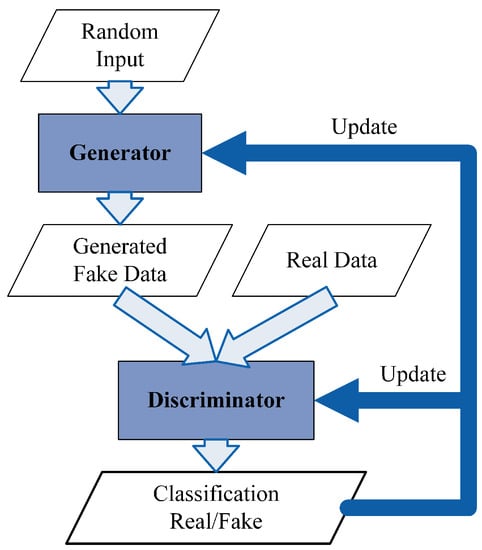
Figure 1.
Generative Adversarial Network.
The generator produces fake data from the random input as illustrated in Figure 1. The discriminator receives two inputs, the real data and the fake data generated by the generator, and produces an output indicating probabilities that samples are real. The two play min-max game with value function :
where G and D are the generator and discriminator, x is the real data sample drawn from , and z is the random (noise) input drawn from .
Studies have demonstrated that GANs can provide good samples [19,20,21]; however, their training may experience diverging or oscillatory behavior resulting in failure to converge [22]. GANs are also prone to mode collapse and vanishing gradients. Mode collapse refers to a situation in which the generator collapses and always produces the same outputs whereas vanishing gradients indicate a situation in which the generator updates become so small that the overall GAN fails to learn [22].
Wasserstein GANs (WGANs) [16] have been proposed to deal with non-convergence and vanishing gradient problems. The cost function in original GANs has a large variance of gradients what makes the model unstable. WGANs improve stability of the training process by using a new cost function, Wasserstein distance, which has smoother gradients everywhere. The Wasserstein distance calculation can be simplified using Kantorovich-Rubinstein duality to:
where and are probability distributions, is the least upper bound, and f is a K-Lipschitz function following the following constraint:
Wasserstein distance in WGAN, uses 1-Lipschitz functions, therefore, the .
Metropolis-Hastings GAN (MH-GAN) [17] aims to improve standard GANs by adding aspects of Markov Chain Monte Carlo. In standard GANs, the discriminator is used solely to train the generator and is discarded upon the end of training. In MH-GAN, the discriminator from GAN training creates a wrapper around the generator. The generator produces a set of samples, and the discriminator chooses the sample closest to the real data distribution. This way, the discriminator contributes to the quality of the generated samples.
2.2. Recurrent Neural Networks
Recurrent Neural Networks (RNNs) [23] are a family of neural networks designed for processing sequential data including time series data such as those found in energy forecasting. While feedforward neural networks only consider the current input to calculate the output, RNNs consider the current input together with all previously received inputs by using recurrent connections that span adjacent time steps. This enables RNNs to capture temporal dependencies.
As illustrated in Figure 2, an RNN takes a sequence of inputs to produce a sequence of outputs . Note that the number of outputs m can be less or equal to the number of inputs n. Hidden states h serve as a mechanism to remember information through time. The output at time step t is obtained as:
where is the current input, is the previous hidden state, and f is a non-linear function.
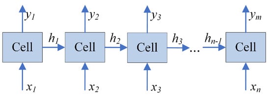
Figure 2.
Recurrent Neural Network.
The cell in Figure 2 can be any RNN cell including vanilla and long short-term memory (LSTM). The back-propagation through time algorithm with the Vanilla RNN cell can lead to the vanishing gradient problem for longer sequences. The LSTM cell was designed to overcome this problem, and, as a result, these models are able to store information for longer periods of time. Figure 2 illustrates a single layer RNN. The stacked RNN, sometimes referred to as multilayer RNN, extends this model by stacking layers of memory cells on top of each other. These additional layers add levels of abstractions and potentially allow the cells at each layer to operate at different time scales [24].
3. Related Work
As our study focuses on generating data for energy forecasting, this section first reviews data sets used in energy forecasting studies and then discusses GAN networks in different domains.
3.1. Data Sets in Energy Forecasting
Amasyali and El-Gohary [25] surveyed energy forecasting studies: 67% of reviewed studies used real data, 19% simulation data, and 14% public benchmark data. This dominance of real data sets demonstrated the importance of historical data and illustrated the need for new and/or larger energy forecasting data sets. While some of the real data used for forecasting are pubic [2], a number of studies deal with private [26] real-world data sets.
In the same work [25], Amasyali and El-Gohary point out that physical models including simulation software such as EnergyPlus, eQUEST, and Ecotect, calculate building energy consumption based on detailed building and environmental parameters, but such detailed information may not always be available. On the other hand, data driven approaches do not require such details about the simulated building, but they require sensors for data collection. From their survey [25], it can be observed that simulation is often used in the design stage while data driven approaches are common in demand and supply management. Physics and data driven approaches do not replace each other; they are applied in different scenarios based on their advantages and disadvantages.
Deb et al. [27] reviewed time series techniques for building energy consumption. They observed that simulation and energy modeling software such as EnergyPlus, IES, eQUEST, and Ecotect have been greatly successful in energy modeling of new buildings. For energy forecasting, when historical data is not available, computer simulations are very effective [27]. However, many factors govern energy consumption including physical properties of building materials, weather, and occupants’ behaviors. Due to complexity of those factors and their interactions, accurate energy forecasting through simulations is challenging [27]. Deb et al. [27] noted that for existing buildings, when historical data is available, data driven techniques such as those based on machine learning and statistics have been more accurate than simulations.
Lazos et al. [28] investigated approaches for incorporating weather conditions into energy forecasting. The three categories of forecasting approaches were considered: statistics, machine learning, and physics(numerical)-based models. While physics models do not require historical data and are able to provide explanations for the forecasts, they are often highly complex and require extensive details about structural characteristics, thermodynamic, operating schedule, and other properties. Lazos et al. [28] also noted that it is challenging to model occupants’ behaviors in physics-based systems. In contrast, data driven approaches do not require such details about the buildings and are capable of capturing some of occupants’ behavior from historical data, but require significant amounts of data.
According to the reviewed studies [25,27,28], simulation can be used for energy forecasting, but machine learning models trained with historical data are much more common. Moreover, synthetic building energy consumption data is especially hard to generate because, in addition to the building properties, use type, and operating schedule, energy consumption also depends on human behavior. Pillai et al. [29] proposed an approach for generating synthetic load profiles using available load and weather data. While Pillai et al. aim to create benchmark profiles, our work generates data for ML. Ngoko et al. [30] generated solar radiation data using Markov models; in contrast, our study is concerned with generating data for energy forecasting.
3.2. Generative Adversarial Networks (GANs)
In recent years, Generative Adversarial Networks (GANs) have seen great progress and received increased attention because of their ability to learn high-dimensional distributions. Originally, GANs were designed for images, and today, the most common use of GAN is in tasks that involve images. For example, works of Mao et al. [19], Denton et al. [20], and Karras et al. [21] deal with generating high quality images: Mao et al. [19] focus on vanishing gradient problem, Denton et al. [20] propose the Laplacian pyramid of adversarial networks for generating high-resolution images, and Karras et al. [21] improve the human-face generation by using style-based generator. StackGAN [14] synthesizes high-quality images from text descriptions by using a two-stage process: first, a low resolution image is created from text descriptions, and then this image with text goes through a refinement process to create photo-realistic details. SRGAN, a GAN for image superresolution (SR) [31] is capable of inferring photo-realistic images with 4× upscaling factors. Zhang et al. [32] used GANs for image de-raining (removing rain from images), consequently improving the visual quality and making images better suited for vision systems.
While the reviewed works [14,19,20,21,31,32] deal with images, our study is concerned with time series data in the energy domain. The possibility to apply GANs with sequential and time-series data has been recognised, and GAN-based approaches have been proposed in different domains and for different tasks. Continuous Recurrent Neural Networks with adversarial training (C-RNN-GAN) [33] have been used for music generation and SeqGAN [34] for text generation. While those works [33,34] deal with discrete sequence generation, the majority of data in the energy domain is real-valued and thus our work is concerned with real-valued data.
Esteban et al. proposed a Recurrent GAN [35] for generating realistic real-valued multi-dimensional time series data focusing on the application to medical data. Similar to our study, the work of Esteban et al. also uses recurrent neural networks for both the generator and discriminator. In contrast to the work of Esteban et al. which uses a GAN similar to the original Goodfellow et al. GAN [13], our approach applies Wasserstein GAN. Moreover, we take advantage of Metropolis-Hastings GAN (MH-GAN) [17] approach for generating new data. The same work [35] proposed “Train on Synthetic, Test on Real” (TSTR) approach for evaluating GANs. TSTR is applicable when a supervised task can be defined over the training data: the basic idea is to use synthetic data generated by GAN to train the model and then test the model on a held-out set from the real data. Our study also employs TSTR as a part of the evaluation process.
EEG-GAN generates electroencephalographic (EEG) brain signal using Wasserstein GANs with gradient penalty (WGAN-GP) [36]. While EEG-GAN employs a convolutional neural network (CNN), our work replaces CNN with RNN because of its ability to model temporal dependencies.
To deal with learning from imbalanced datasets, Douzas and Bacao [37] applied GANs to generating artificial data for the minority classes. Their experiments show an improvement in the quality of data when GANs are used in place of oversampling algorithms such as SMOTE (synthetic minority over-sampling technique). MisGAN, a GAN-based framework for learning from complex, high-dimensional incomplete data [38], was proposed for the task of imputing missing data. VIGAN [39] also deals with imputation, but in this case with scenarios when certain samples miss an entire view of data. While Douzas and Bacao [37], Li et al. [38], and Shang et al. [39] generate specific part of data (imbalanced classes or missing data), our work deals with generating new energy data samples for training ML models.
Another category of works important to discuss here consists of those related to the GAN evaluation. With image GANs, evaluation often involves visual inspection of the generated sample; however, this is more difficult to do with time-series data. Inception score (IS) has been proposed for evaluating image generative models [40]; IS uses Inception network pre-trained on ImageNet data set to calculate the score. Nevertheless, not only is IS not applicable for non-image data, it is also incapable of detecting overfitting [41].
Sajjadi et al. [42] proposed precision and recall for distributions. Precision measures how much of distribution Q can be generated by a part of reference distribution P while recall measures how much of P can be generated by a part of Q. By using a two-dimensional score, they are able to distinguish between the quality of generated images from the coverage of the reference distribution. Still, their study [42] was primarily concerned with images.
Theis et al. [43] compared different evaluation approaches and concluded that different metrics have different trade-offs and favour different models. They highlight the importance of matching training and evaluation to the target application. As the main objective of our work is to generate electricity data suitable for training machine learning models, the evaluation is performed in the context of the application by assessing the suitability of the generated data for ML task. Specifically, this is done by training the prediction model on the generated data and testing it on the real data.
4. Methodology
Figure 3 depicts the overview of the R-GAN approach. As R-GANs use RNNs for the generator and discriminator, data first needs to be pre-processed to accommodate the RNN architecture. Accordingly, this section first describes data pre-processing consisting of feature engineering (ARIMA and Fourier transform), normalization, and sample generation (sliding window). Next, R-GAN is described and the evaluation process is introduced.
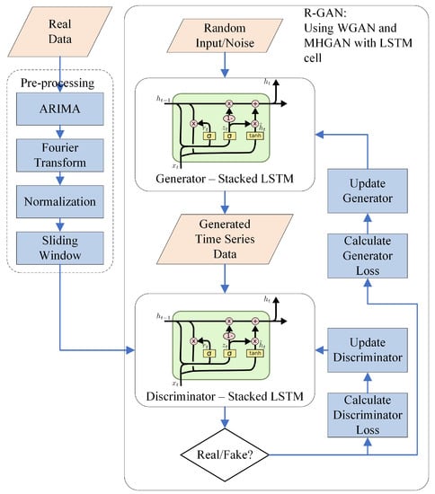
Figure 3.
Recurrent Generative Adversarial Networks (GAN) for Energy Data.
4.1. Data Pre-Processing
In this paper, the term core features refers to energy consumption features and any other features present in the original data set (e.g., reading hour, weekend/weekday). In the data pre-processing step, these core features are first enriched through feature engineering using auto regressive integrated moving average (ARIMA) and Fourier transform (FT). Next, all features are normalized and the sliding window technique is applied to generate samples for GAN training.
4.1.1. ARIMA
Auto regressive integrated moving average (ARIMA) [44] models are fitted to time series data to better understand the data or to forecast future values in the time series. The auto regressive (AR) part models the variable of interest as regression of its own past values, the moving average (MA) part uses a linear combination of past error terms for modeling, and Integrated (I) refers to dealing with non-stationarity.
Here, ARIMA is used because of its ability to capture different temporal structures in time series data. As this work is focused on generating energy data, the ARIMA model is fitted to the energy feature. The values obtained from the fitted ARIMA model are added as a new engineered feature to the existing data set. The RNN itself is capable of capturing temporal dependencies, but adding ARIMA further enhances time modeling and, consequently, improves the quality of the generated data as will be demonstrated in Section 5.
4.1.2. Fourier Transform
Fourier transform (FT) decomposes a time signal into its constituent frequency domain representations [44]. Using FT, every waveform can be represented as the sum of sinusoidal functions. An inverse Fourier transform synthesizes the original signal from its frequency domain representations. Because FT identifies which frequencies are present in the original signal, FT is suitable for discovering cycles in the data.
Like with ARIMA, only the energy feature is used with FT. The energy time series is decomposed into sinusoidal representations, n dominant frequencies are selected, and a new time series is constructed using these n constituent signals. This new time series represents a new feature. When the number of components n is low, the new time series only captures the most dominant cycles, whereas for a large number of components, the created time series approaches the original time series. One value of n creates one new feature, but several values with their corresponding features are used in order to capture different temporal scales.
The objective of using FT is similar to the one of ARIMA: to capture time dependencies and, consequently, improve quality of the generated data. The experiments demonstrate that both ARIMA and Fourier transform contribute to the quality of the generated data.
4.1.3. Normalization
To bring the values of all features to a similar scale, the data was normalized using normalization. The values of each feature were scaled to values between 0 and 1 as follows:
where x is the original value, and are the minimum and maximum of that feature vector, and is the normalized value.
4.1.4. Sliding Window
At this point, data is still in a matrix format as illustrated in Figure 4 with each row containing readings for a single time step. Note that features in this matrix include all features contained in the original data set (core features) such as appliance status or the day of the week, as well as additional features engineered with ARIMA and FT.
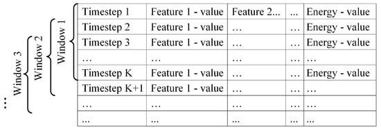
Figure 4.
Sliding Window Approach.
As the generator core is RNN, samples need to be prepared into a form suitable for RNN. To do this, the sliding window technique is applied. As illustrated in Figure 4, the first K rows correspond to the first time window and make the first training sample. Then, the window slides for S steps, and the readings from the time step S to make the second sample. Note that in Figure 4, the step is although other step sizes could be used. Each sample is a matrix of dimension , where K is the window length and F is the number of features.
4.2. R-GAN
Similar to an image GAN, R-GAN consists of the generator and the discriminator as illustrated in Figure 3. However, while an image GAN typically uses CNN for the generator and discriminator, R-GAN substitutes CNN with the stacked LSTM and a single dense layer. The architectures of the R-GAN generator and discriminator are shown in Figure 5. The stacked LSTMs were selected because the LSTM cells are able to store information for longer sequences than Vanilla RNN cells. Moreover, stacked hidden layers allow capturing patterns at different time scales.
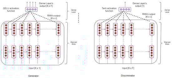
Figure 5.
Recurrent GAN (R-GAN) generator and discriminator.
Both the generator and discriminator have a similar architecture consisting of stacked LSTM and a dense layer (Figure 5), but they differ in dimensions of their inputs and outputs because they serve a different purpose: one generates data and the other one classifies samples into fake and real. The generator takes random inputs from the predefined Gaussian latent space and generates time series data. The input has the same dimension as the siding window length K. The RNN output before the fully connected later has dimension (window length × cell state dimension). The generated data (generator output) has the same dimensions as the real data after pre-processing: each sample is of dimension (window length × number of features).
GELU (Gaussian error linear unit) activation function has been selected for the generator and discriminator RNNs [45] as it recently outperformed rectified linear unit (ReLU) and other activation functions [45]. The GELU can be approximated by [45]:
Similar to the ReLU (rectified linear unit) and the ELU (exponential linear unit ) activation functions, GELU enables faster and better convergence of neural networks than the sigmoid function. Moreover, GELU merges ReLU functionality and dropout by multiplying the neuron input by zero or one, but this dropout multiplication is dependent on the input: there is a higher probability of the input to be dropped as the input value decreases [45]. The stacked RNN is followed by the dense layer in both the generator and discriminator. The dense layer activation function for the generator is GELU because of the same reasons explained with GELU selection in a stacked RNN. In the discriminator, the dense layer activation function is tanh to achieve real/synthetic classifications.
As illustrated in Figure 3, the generated data together with pre-processed data are passed to the discriminator which learns to differentiate between real and fake samples. After a mini-batch consisting of several real and generated samples is processed, discriminator loss is calculated and the discriminator weights are updated using gradient descent. As R-GAN uses WGAN, the updates are done slightly differently than in the original GAN. In the original GAN work [13], each discriminator update is followed by the generator update. In contrast, the WGAN algorithm trains the discriminator relatively well before each generator update. Consequently, in Figure 3, there are several discriminator update loops before each generator update.
Once the generator and discriminator are trained, the R-GAN is ready to generate data. At this step, typically only the trained generator is used. If the generator was trained perfectly, the resulting generated distribution, , would be the same as the real one. Unfortunately, GANs may not always converge to the true data distribution, thus taking samples directly from these imperfect generators can produce low quality samples. However, our work takes advantage of the Metropolis-Hastings GAN (MH-GAN) approach [17] in which both the generator and discriminator play roles in generating samples.
Data generation using MH-GAN approach is illustrated in Figure 6. The discriminator, together with the trained generator G, forms a new generator . The generator G takes as input random samples and produces time series samples . Some of the generated samples are closer to the real data distribution than the others. The discriminator serves as a selector to choose the best sample x from the set . The final output is the generated time series sample x.
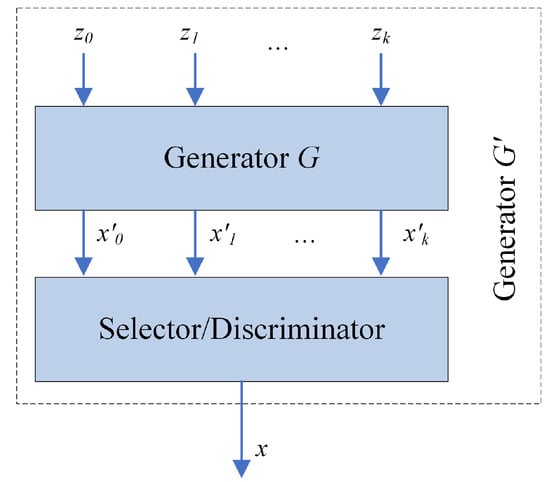
Figure 6.
Metropolis-Hastings GAN (MH-GAN) approach.
4.3. Evaluation Process
The main objective of this work is to generate data for training ML models; therefore, the presented R-GAN is evaluated by assessing the quality of ML models trained with synthetic data. As energy forecasting is a common ML task, it is used here for the evaluation too. In addition to Train on Synthetic, Test on Real (TSTR) and Train on Real, Test on Synthetic (TRTS) approaches proposed by Esteban et al. [35], two additional metrics are employed: Train on Real, Test on Real (TRTR) and Train on Synthetic, Test on Synthetic (TSTS).
Train on Synthetic, Test on Real (TSTR): A prediction model is trained with synthetic data and tested on real data. TSTR was proposed by Esteban et al. [35]: they evaluated the GAN model on a clustering task using random forest classifier. In contrast, our study evaluates R-GAN on an energy forecasting task using an RNN forecasting model. Note that this forecasting RNN is different than RNNs used for the GAN generator and discriminator, and could be replaced by a different ML algorithm. RNN was selected because of its recent success in energy forecasting studies [26]. This forecasting RNN is trained with synthetic data and tested on real data.
Consequently, TSTR evaluates the ability of the synthetic data to be used for training energy forecasting models. If the R-GAN suffers from the mode collapse, TSTR degrades because the generated data do not capture diversity or real data and, consequently, the prediction model does not capture this diversity.
Train on Real, Test on Synthetic (TRTS): This is the reverse of TSTR: a model is trained on the real data and tested on the synthetic data. The process is exactly the same as in TSTR with exception of reversed roles of synthetic and real data. TRTS serves as an evaluation of GAN’s ability to generate realistic looking data. Unlike TSTR, TRTS is not affected by the mode collapse as a limited diversity of synthetic data does not affect forecasting accuracy. As the aim is to generate data for training ML models, TSTR is a more significant metrics than TRTS.
Train on Real, Test on Real (TRTR): This is a traditional evaluation with the model trained and tested on the real data (with separate train and test sets). TRTR does not evaluate the synthetic data itself, but it allows for the comparison of accuracy achieved when a model is trained with real and with synthetic data. Low TRTR and TSTR accuracies indicate that the forecasting model is not capable of capturing variations in data and do not imply low quality of synthetic data. The goal of the presented R-GAN data generation is the TSTR value comparable to the TRTR value, regardless of their absolute values: this demonstrates that the model trained using synthetic data has similar abilities as the model trained with real data.
Train on Synthetic, Test on Synthetic (TSTS): Similar to TRTR, TSTS evaluates the ability of the forecasting model to capture variations in data: TRTR evaluates the accuracy with real data and TSTS with synthetic data. Large discrepancies between TRTR and TSTS indicate that the model is much better with real data than with synthetic, or the other way around. Consequently, this means that the synthetic data does not reassemble the real data.
5. Evaluation
5.1. Data sets and Pre-Processing
The evaluation was carried out on two data sets: UCI (University of California, Irvine) appliances energy prediction data set [46] and Building Data Genome set [6]. UCI data set consists of energy consumption readings for different appliances with additional attributes such as temperature and humidity. The reading interval is 10 min and the total number of samples is 19,736. Day of the week and month of the year features were created from reading date/time, resulting in a total of 28 features.
Building Data Genome set contains one year of hourly, whole building electrical meter data for non-residential buildings. In experiments, readings from a single building were used; thus, the number of samples is 24 × 365 = 8760. With this data set, energy consumption, year, month, day of the year, and hour of the day features were used.
For both data sets, the process is the same. The data set is pre-processed as described in Section 4.1. ARIMA is applied first to create an additional feature: to illustrate this step, Figure 7 shows original data (energy consumption feature) and ARIMA fitted model for UCI data set.
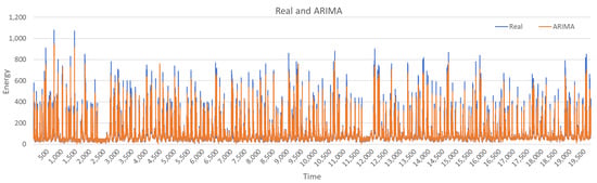
Figure 7.
Auto Regressive Integrated Moving Average (ARIMA) fitted model (UCI data set).
Next, Fourier transform (FT) is applied. FT can be used with a different number of components resulting in different signal representations; in the experiments, four transformations were considered with 1, 10, 100, and 1000 components. The four representations are illustrated in Figure 8 on UCI data set. It can be observed that one component results in almost constant values and 10 components capture only large scale trends. As the number of components increases to 100 and 1000, more smaller-scale changes are captured and the representation is closer to the original data. These four transformations with 1, 10, 100, and 1000 components make the four additional features.
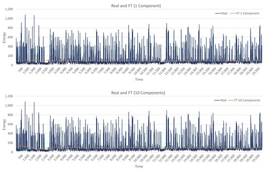
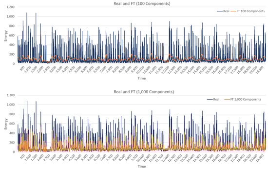
Figure 8.
The results of Fourier transform with 1, 10, 100, and 1000 components (UCI data set).
At this point, all needed additional features are generated (total of 33 features), and the pre-processing continues with normalization (Figure 3). To prepare data for RNN, the sliding window technique is applied with the window length indicating that 60 time steps make one sample, and step specifying that the window slides for 30 time steps to generate the next sample. This window size and step were determined from the initial experiments.
5.2. Experiments
The R-GAN was implemented in Python with Tensorflow library [47]. The experiments were performed on a computer with Ubuntu OS, AMD Ryzen 4.20 GHz processor, 128 GB DIMM RAM, and four NVIDIA GeForce RTX 2080 Ti 11GB graphics cards. Training the proposed R-GAN is computationally expensive; therefore, GPU acceleration was used. However, once the model is trained, it does not require significant resources and CPU processing is sufficient.
Both discriminator and generator were stacked LSTMs with the hyperparameters as follows:
- Number of layers
- Cell state dimension size
- Learning rate =
- Batch size = 100
- Optimizer = Adam
The input to the generator consisted of samples of size 60 (to match the window length) drawn from the Gaussian distribution. The generator output was of size (window length × number of features). The discriminator input was of the same dimension as the generator output and the pre-processed real data.
Hyperparameters were selected according to the hyperparameter studies, commonly used settings, or by performing experiments. Keskar et al. [48] observed that performance degrades for batch sizes larger than commonly used 32–521. To keep in that range, and to be close to the original WGAN work [16], batch size 100 was used. For each batch, 100 generated synthetic samples and 100 randomly selected real samples were passed to the discriminator for classification. Increasing the cell state dimension typically leads to the increased LSTM accuracy, but also increases the training time [49]; thus, moderate 128 size was selected.
Greff et al. [49] observed that the learning rate is the most important LSTM parameter and that there is often a large range (up to two orders of magnitude) of good learning rates. Figure 9 shows generator and discriminator loss for the learning rates (LR) , , and for UCI data set and the model with ARIMA and FT features. Similar patterns have been observed with Building Genome data, therefore, here we only discuss loss for UCI experiments. The generator and discriminator are competing against each other; thus, improvement in one results in a decline in the other until the other learns to handle the change and causes the decline of its competitor. Hence, in the graph, oscillations are observed indicating that the networks are trying to learn and beat the competitor. For learning rate , the generator stabilizes quite well, while the discriminator shows fluctuations as it tries to defeat the generator. Oscillations of the objective function are quite common in GANs, and WGAN is used in this work to help with convergence. Nevertheless, as the learning rate increases to and , the generator and discriminator are experiencing increased instabilities. Consequently, learning rate was used for the experiments presented in this paper. Additional hyperparameter tuning has a potential to further improve archived results.
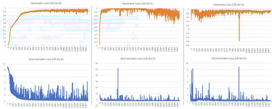
Figure 9.
Generator and discriminator loss for LR = , , and (UCI data set).
All experiments were carried out with 1500 epochs to allow sufficient time for the system to converge. As can be seen from Figure 9, for learning rate , the generator largely stabilizes after around 500 epochs and experiences very little change after 1,000 epochs. At the same time, the discriminator experiences similar oscillation patterns from around 400 epochs onward. Thus, training for 1000 epochs might be sufficient; nevertheless, 1500 epochs allow a chance for further improvements.
R-GAN was evaluated with the four models corresponding to the four sets of features:
- Core features only.
- Core and ARIMA generated features.
- Core and FT generated features.
- Core, ARIMA, and FT generated features.
As described in Section 4.3, ML task, specifically energy forecasting, was used for the evaluation with TRTS, TRTR, TSTS, and TSTR metrics. Forecasting models for those evaluations were also RNNs. Forecasting model hyperparameters for each experiment were tuned using the expected improvement criterion according to Bergstra et al. [50], which results in different hyperparameters for each set of input features. This way, we ensure that the forecasting model is tuned for the specific use scenario. The following ranges of hyperparameters were considered for the forecasting model:
- Hidden layer sizes: 32, 64, 128
- Number of layers: 1, 2
- Batch sizes: 1, 5, 10, 15, 30, 50
- Learning rates: continuous from 0.001 to 0.03
For each of R-GAN models, 7200 samples were generated and then TSTR, TRTS, TRTR, an TSTS approaches with an RNN prediction model were applied. Mean absolute percentage error (MAPE) and mean absolute error (MAE) were selected as evaluation metrics because of their frequent use in energy forecasting studies [51,52]. They are calculated as:
where y is the actual value, is the predicted value, and N is the number of samples.
5.3. Results and Discussion—UCI Data Set
This subsection presents results achieved on UCI data set and discusses findings. MAPE and MAE for the four evaluations TRTS, TRTR, TSTR, and TSTS are presented in Table 1. For the ease of the comparison, the same data is presented in a graph form: Figure 10 compares models based on MAPE and Figure 11 based on MAE.

Table 1.
Train on Real, Test on Synthetic (TRTS), Train on Real, Test on Real (TRTR), Train on Synthetic, Test on Real (TSTR), and Train on Synthetic, Test on Synthetic (TSTS) accuracy for R-GAN (UCI data set).
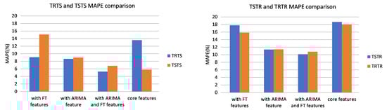
Figure 10.
MAPE(%) comparison between TRTS/TSTS and TSTR/TRTR (UCI data set).
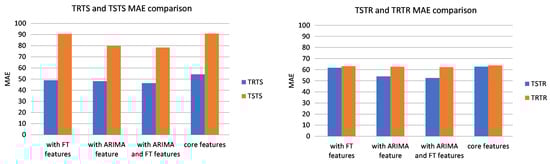
Figure 11.
MAE comparison between TRTS/TSTS and TSTR/TRTR (UCI data set).
As we are interested in using synthetic data for training ML models, TSTR is a crucial metric. In terms of TSTR, addition of ARIMA and FT features to the core features reduces MAPE from 18.67% to 10.12% and MAE from 62.74 to 52.54. Moreover, it can be observed that for all experiments adding ARIMA and FT features improves the accuracy in terms of both MAPE and MAE.
Because forecasting models always result in some forecasting errors even when trained with real data, it is important to compare the accuracy of the model trained with synthetic data with the one trained with the real data. TRTR evaluates the quality of the forecasting model itself. As can be observed from Table 1, TSTR accuracy is close to TRTR accuracy for all models irrelevant of the number of features. This indicates that the accuracy of the forecasting model trained with synthetic data is close to the accuracy of the model trained with real data. When the model is trained with real data (TRTR), the MAPE for the model with all features is 10.81% whereas when trained with synthetic data (TRTS) MAPE is 10.12%. Consequently, comparable TSTR and TRTR values demonstrate the usability of synthetic data for ML training.
The accuracy of TSTR is higher than the accuracy of TRTS in terms of both MAPE and MAE for all experiments. Good TRTS accuracy shows that the predictor is able to generalize from real data and that generated samples are similar to real data. However, higher TSTR errors than TRTS errors indicate that the model trained with generated data does not capture the real data as well as the model trained on the real data. A possible reason for this is that, in spite of using techniques for dealing with mode collapse, the variety of generated samples is still not as high as the variety of real data.
Visual comparison cannot be done in a similar way as in image GANs, but Figure 12 shows examples of two generated samples compared with the most similar real data samples. It can be observed that the generated patterns are similar, but not the same as the real samples; thus, data looks realistic without being a mere repetition of the training patterns. Although Figure 12 provides some insight into generated data, already discussed TSTR and its comparison to TRTR are the main metrics evaluating the usability of generated data for ML training.
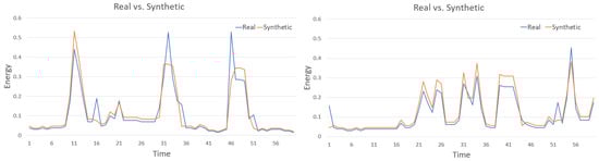
Figure 12.
Two examples of generated data samples compared to real data.
To further compare real and synthetic data, statistical tests were applied to evaluate if there is a statistically significant difference between the generated and real data distributions. The Kruskal-Wallis H test also referred to “one-way ANOVA on ranks”, and the Mann-Whitney U test were used because both of them are non-parametric tests and do not assume normally distributed data. The parametric equivalent of the Kruskal-Wallis H test is one-way ANOVA (analysis of variance). The null hypothesis for the statistical tests was: the distributions of the real and synthetic populations are equal. The H values and U values together with the corresponding p values for each test and for each of the GAN models are shown in Table 2. Each test compares the real data with the synthetic data generated with one of the four models. The level of significance was considered.
Table 2.
Kruskal-Wallis H Test and Mann-Whitney U test (UCI data set).
As the p value for each test is greater than , the null hypothesis is confirmed: for each of the four synthetic data sets, irrelevant of the number of features, there is little to no evidence that the distribution of the generated data is statistically different than the distribution of the real data. H and U tests provide evidence about the similarity of distributions; nevertheless, TSTR and TRTR remain the main metrics for comparing among the GAN models.
Note the intuitive similarity between reasoning behind R-GAN and a common approach for dealing with the class imbalance problem, SMOTE (Synthetic Minority Over-sampling TEchnique) [53]. SMOTE takes each minority class sample and creates synthetic samples on lines connecting any/all of the k minority neighbors. Although R-GAN deals with the regression problem and SMOTE with classification, both create new samples by using knowledge about existing samples. SMOTE does so by putting new samples between existing (real) ones whereas R-GAN learns from the real data, and then it is able to generate samples similar to the real ones. Consequently, R-GAN has a potential to be used for class imbalance problems.
Overall, the results are promising as the forecasting model trained on the synthetic data is achieving similar forecasting accuracy as the one trained on the real data. As illustrated in Table 1, both MAPE and MAE for the model trained on the synthetic and tested on the real data (TSTR) are close to MAPE and MAE for the model trained and tested on the real data (TRTR).
5.4. Results and Discussion—Building Genome Data Set
This subsection presents the results achieved with Building Genome data. MAPE and MAE for the four evaluations TRTS, TRTR, TSTR, and TSTS are presented in Table 3. The same data is displayed in a graph form for ease of comparison: Figure 13 compares models based on MAPE and Figure 14 based on MAE.
Table 3.
TRTS, TRTR, TSTR, and TSTS accuracy for R-GAN (Building Genome data set).
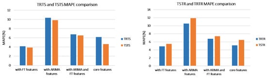
Figure 13.
Mean Absolute Percentage Error (MAPE)(%) comparison between TRTS/TSTS and TSTR/TRTR (Building Genome data set).
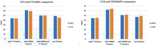
Figure 14.
Mean Absolute Error (MAE) comparison between TRTS/TSTS and TSTR/TRTR (Building Genome data set).
Similar to the UCI data set, TSTR accuracy is close to TRTR accuracy in terms of both, MAPE and MAE, for all models, irrelevant of the number of features. As in the UCI experiments, this indicates that the accuracy of the forecasting model trained with synthetic data is close to the accuracy of the model trained with real data. The best model was with core and FT features: it achieved the MAPE of 4.86% when trained with real data (TRTR) and 5.49% when trained with synthetic data (TSTR).
While with UCI data set, the model with FT and ARIMA features achieved the best results, with Building Genome data, the model with FT (without ARIMA) achieved the best result over all metrics. Note that this is the case even when the model is trained and tested on the real data (TRTR) without any involvement of the generated data: with ARIMA and FT, TRTR MAPE was 6.77% whereas with FT only, MAPE was 4.87%. Thus, this degradation of the model with addition of ARIMA is a consequence of the data set itself and not the result of data generation.
Analyses of the ARIMA feature in the two data sets showed that the Pearson-Correlation between energy consumption and the ARIMA feature was very different for the two data sets. For Building Genome data, the correlation was 0.987 and for UCI data set it was 0.75, indicating a very high linear correlation between the ARIMA and consumption features in Building Genome data. In Building Genome data set, ARIMA was able to model the patterns of the data much better what indicates that the temporal patterns were much more consistent than it was the case with UCI data set. This pattern regularity also explains higher TRTR accuracy of Building Genome models than UCI models: the best TRTR MAPE for Building Genome was 4.86% and for UCI data set it was 10.81%.
High multicollinearity can indicate redundancy of the feature set and can lead to instability of the model and degraded performance [54,55,56]. One way of dealing with multicollinearity is feature selection [55] which will remove unnecessary features. With such a high correlation in Building Genome data, removal of one of the correlated features is expected to improve performance as confirmed in our experiments with the model without the ARIMA feature performing better. This could be remedied through feature selection [55]. As the aim of our work is not to improve the accuracy of the forecasting models, but to explore generating synthetic data for machine learning, feature selection is not considered.
From Table 1 and Table 3, it can be observed that, as with UCI data set, for Building Genome data set TSTR errors are higher than TRTS errors in terms of both, MAPE and MAE, for all experiments. As noted with UCI experiments, this could be caused by the variety of generated samples not being as high as the variety of real data.
Two statistical tests, the Kruskal-Wallis H test and the Mann-Whitney U test, were applied to evaluate if there is a statistically significant difference between the synthetic and real data. Again, the null hypothesis was: the distributions of the real and synthetic populations are equal. Table 4 shows H values and U values together with the corresponding p values for each test and for each of the GAN models. The same level of significance was considered.
Table 4.
Kruskal-Wallis H Test and Mann-Whitney U test (Building Genome data set).
For Building Genome experiments, same as for UCI experiments, the p value for each test is greater than and the null hypothesis is confirmed: for each of the four synthetic data sets, irrelevant of the number of features, there is little to no evidence that the distribution of the generated data is statistically different than the distribution of the real data.
Overall, the results for both data sets, UCI and Building Genome data set, exhibit similar trends. As illustrated in Table 1 and Table 3, accuracy measures, MAPE and MAE, for the models trained on the synthetics data and tested on the real data (TSTR) are close to MAPE and MAE for the model trained and tested on the real data (TRTR) indicating suitability of generated data for training ML models.
6. Conclusions
Machine learning (ML) has been used for various smart grid tasks, and it is expected that ML role will increase as new technologies emerge. Those ML applications typically require significant quantities of historical data; however, those historical data may not be readily available because of challenges and costs associated collecting data, privacy and security concerns, or other reasons.
This paper investigates generating energy data for machine learning taking advantage of Generative Adversarial Networks (GANs) typically used for generating realistic-looking images. Introduced Recurrent GAN (R-GAN) replaces Convolutional Neural Networks (CNNs) used in image GANs with Recurrent Neural Networks (RNNs) because of RNNs ability to capture temporal dependence in time series data. To deal with convergence instability and to improve the quality of generated data, Wasserstein GANs (WGANs) and Metropolis-Hastings GAN (MH-GAN) techniques were used. Moreover, ARIMA and Fourier Transform were applied to generate new features and, consequently, improve the quality of generated data.
To evaluate the suitability of data generated with R-GANs for machine learning, energy forecasting experiments were conducted. Synthetic data produced with R-GAN was used to train the energy forecasting model and then, the trained model was tested on the real data. Results show that the model trained with synthetic data achieves similar accuracy as the one trained with real data. The addition of features generated by ARIMA and Fourier transform improves the quality of generated data.
Future work will explore the impact of reducing training set size on the quality of the generated data. Also, replacing LSTM with Gated Recurrent Unit (GRU) and further R-GAN tuning will be investigated.
Author Contributions
Conceptualization, M.N.F.; methodology, M.N.F. and K.G.; software, A.M.G. and M.N.F.; validation, A.M.G. and M.N.F.; formal analysis, M.N.F. and K.G.; investigation, A.M.G. and M.N.F.; resources, K.G.; data curation, A.M.G.; writing—original draft preparation, A.M.G. and M.N.F.; writing—review and editing, K.G.; visualization, A.M.G. and M.N.F.; supervision, K.G.; project administration, K.G.; funding acquisition, K.G. All authors have read and agreed to the published version of the manuscript.
Funding
This research was funded by Natural Sciences and Engineering Research Council of Canada under grant number RGPIN-2018-06222.
Conflicts of Interest
The authors declare no conflict of interest.
Abbreviations
The following abbreviations are used in this manuscript:
| AMI | Advanced Metering Infrastructure |
| ARIMA | AutoRegressive Integrated Moving Average |
| C-RNN-GAN | Continuous recurrent GAN |
| CNN | Convolutional Neural Network |
| DL | Deep Learning |
| EEG | electroencephalographic brain signal |
| EEG-GAN | GAN for generating EEG |
| ELU | Exponential Linear Unit |
| FT | Fourier Transform |
| LSTM | Long Short-Term Memory |
| LR | Learning Rate |
| GAN | Generative Adversarial Network |
| GELU | Gaussian Error Linear Unit |
| GRU | Gated Recurrent Unit |
| MAPE | Mean Absolute Percentage Error |
| MAE | Mean Absolute Error (MAE) |
| ML | Machine Learning |
| MH-GAN | Metropolis-Hastings GA |
| NILM | Nonintrusive Load Monitoring |
| R-GAN | Recurrent GAN |
| ReLU | Rectified Linear Unit |
| RNN | Recurrent Neural Network |
| SMOTE | Synthetic Minority Over-sampling TEchnique |
| SR | image superresolution (SR) |
| SRGAN | GAN for image superresolution (SR) |
| TRTR | Train on Real, Test on Real |
| TRTS | Train on Real, Test Synthetic |
| TSTR | Train on Synthetic, Test on Real |
| TSTS | Train on Synthetic, Test on Synthetic |
| WGAN | Wasserstein GAN |
| WGAN-GP | Wasserstein GAN with gradient penalty |
References
- Zhou, K.; Fu, C.; Yang, S. Big data driven smart energy management: From big data to big insights. Renew. Sustain. Energ Rev. 2016, 56, 215–225. [Google Scholar] [CrossRef]
- Tian, Y.; Sehovac, L.; Grolinger, K. Similarity-based chained transfer learning for energy forecasting with Big Data. IEEE Access 2019, 7, 139895–139908. [Google Scholar] [CrossRef]
- Sial, A.; Singh, A.; Mahanti, A.; Gong, M. Heuristics-Based Detection of Abnormal Energy Consumption. In Smart Grid and Innovative Frontiers in Telecommunications, Proceedings of the International Conference on Smart Grid Inspired Future Technologies, Auckland, New Zealand, 23–24 April 2018; Springer: Berlin, Germany, 2018; pp. 21–31. [Google Scholar]
- Sial, A.; Singh, A.; Mahanti, A. Detecting anomalous energy consumption using contextual analysis of smart meter data. In Wireless Networks; Springer: Berlin, Germany, 2019; pp. 1–18. [Google Scholar]
- Deb, C.; Frei, M.; Hofer, J.; Schlueter, A. Automated load disaggregation for residences with electrical resistance heating. Energy Build. 2019, 182, 61–74. [Google Scholar] [CrossRef]
- Miller, C.; Meggers, F. The Building Data Genome Project: An open, public data set from non-residential building electrical meters. Energy Proc. 2017, 122, 439–444. [Google Scholar] [CrossRef]
- Ratnam, E.L.; Weller, S.R.; Kellett, C.M.; Murray, A.T. Residential load and rooftop PV generation: An Australian distribution network dataset. Int. J. Sustain. Energy 2017, 36, 787–806. [Google Scholar] [CrossRef]
- Wang, Y.; Chen, Q.; Hong, T.; Kang, C. Review of smart meter data analytics: Applications, methodologies, and challenges. IEEE Trans. Smart Grid 2018, 10, 3125–3148. [Google Scholar] [CrossRef]
- Guan, Z.; Li, J.; Wu, L.; Zhang, Y.; Wu, J.; Du, X. Achieving Efficient and Secure Data Acquisition for Cloud-Supported Internet of Things in Smart Grid. IEEE Internet Things 2017, 4, 1934–1944. [Google Scholar] [CrossRef]
- Liu, Y.; Guo, W.; Fan, C.I.; Chang, L.; Cheng, C. A practical privacy-preserving data aggregation (3PDA) scheme for smart grid. IEEE Trans. Ind. Inform. 2018, 15, 1767–1774. [Google Scholar] [CrossRef]
- Fan, C.; Xiao, F.; Li, Z.; Wang, J. Unsupervised data analytics in mining big building operational data for energy efficiency enhancement: A review. Energy Build. 2018, 159, 296–308. [Google Scholar] [CrossRef]
- Genes, C.; Esnaola, I.; Perlaza, S.M.; Ochoa, L.F.; Coca, D. Robust recovery of missing data in electricity distribution systems. IEEE Trans. Smart Grid 2018, 10, 4057–4067. [Google Scholar] [CrossRef]
- Goodfellow, I.; Pouget-Abadie, J.; Mirza, M.; Xu, B.; Warde-Farley, D.; Ozair, S.; Courville, A.; Bengio, Y. Generative adversarial nets. In Proceedings of the Advances in Neural Information Processing Systems, Montreal, QC, Canada, 8–13 December 2014; pp. 2672–2680. [Google Scholar]
- Zhang, H.; Xu, T.; Li, H.; Zhang, S.; Wang, X.; Huang, X.; Metaxas, D.N. StackGAN: Text to photo-realistic image synthesis with stacked generative adversarial networks. In Proceedings of the IEEE International Conference on Computer Vision, Venice, Italy, 22–29 October 2017; pp. 5907–5915. [Google Scholar]
- Cai, J.; Hu, H.; Shan, S.; Chen, X. FCSR-GAN: End-to-end Learning for Joint Face Completion and Super-resolution. In Proceedings of the IEEE International Conference on Automatic Face & Gesture Recognition, Lille, France, 14–18 May 2019; pp. 1–8. [Google Scholar]
- Arjovsky, M.; Chintala, S.; Bottou, L. Wasserstein GAN. arXiv 2017, arXiv:1701.07875. [Google Scholar]
- Turner, R.; Hung, J.; Frank, E.; Saatchi, Y.; Yosinski, J. Metropolis-Hastings Generative Adversarial Networks. In Proceedings of the International Conference on Machine Learning, Siena, Italy, 10–13 September 2019; pp. 6345–6353. [Google Scholar]
- Xu, T.; Zhang, P.; Huang, Q.; Zhang, H.; Gan, Z.; Huang, X.; He, X. AttnGAN: Fine-grained text to image generation with attentional generative adversarial networks. In Proceedings of the IEEE Conference on Computer Vision and Pattern Recognition, Salt Lake City, UT, USA, 18–22 June 2018; pp. 1316–1324. [Google Scholar]
- Mao, X.; Li, Q.; Xie, H.; Lau, R.Y.; Wang, Z.; Paul Smolley, S. Least squares generative adversarial networks. In Proceedings of the IEEE International Conference on Computer Vision, Venice, Italy, 22–29 October 2017; pp. 2794–2802. [Google Scholar]
- Denton, E.L.; Chintala, S.; Fergus, R. Deep generative image models using a laplacian pyramid of adversarial networks. In Proceedings of the Advances in Neural Information Processing Systems, Montreal, QC, Canada, 7–12 December 2015; pp. 1486–1494. [Google Scholar]
- Karras, T.; Laine, S.; Aila, T. A style-based generator architecture for generative adversarial networks. In Proceedings of the IEEE Conference on Computer Vision and Pattern Recognition, Long Beach, CA, USA, 16–20 June 2019; pp. 4401–4410. [Google Scholar]
- Arjovsky, M.; Bottou, L. Towards principled methods for training generative adversarial networks. In Proceedings of the International Conference on Learning Representations, Toulon, France, 24–26 April 2017. [Google Scholar]
- Goodfellow, I.; Bengio, Y.; Courville, A. Deep Learning; MIT Press: Cambridge, MA, USA, 2016. [Google Scholar]
- Pascanu, R.; Gulcehre, C.; Cho, K.; Bengio, Y. How to construct deep recurrent neural networks. In Proceedings of the Second International Conference on Learning Representations, Banff, AB, Canada, 14–16 April 2014. [Google Scholar]
- Amasyali, K.; El-Gohary, N.M. A review of data-driven building energy consumption prediction studies. Renew. Sustain. Energ Rev. 2018, 81, 1192–1205. [Google Scholar] [CrossRef]
- Sehovac, L.; Nesen, C.; Grolinger, K. Forecasting Building Energy Consumption with Deep Learning: A Sequence to Sequence Approach. In Proceedings of the IEEE International Congress on Internet of Things, Aarhus, Denmark, 17–21 June 2019. [Google Scholar]
- Deb, C.; Zhang, F.; Yang, J.; Lee, S.E.; Shah, K.W. A review on time series forecasting techniques for building energy consumption. Renew. Sustain. Energ Rev. 2017, 74, 902–924. [Google Scholar] [CrossRef]
- Lazos, D.; Sproul, A.B.; Kay, M. Optimisation of energy management in commercial buildings with weather forecasting inputs: A review. Renew. Sustain. Energ Rev. 2014, 39, 587–603. [Google Scholar] [CrossRef]
- Pillai, G.G.; Putrus, G.A.; Pearsall, N.M. Generation of synthetic benchmark electrical load profiles using publicly available load and weather data. Int. J. Electr. Power 2014, 61, 1–10. [Google Scholar] [CrossRef]
- Ngoko, B.; Sugihara, H.; Funaki, T. Synthetic generation of high temporal resolution solar radiation data using Markov models. Sol. Energy 2014, 103, 160–170. [Google Scholar] [CrossRef]
- Ledig, C.; Theis, L.; Huszár, F.; Caballero, J.; Cunningham, A.; Acosta, A.; Aitken, A.; Tejani, A.; Totz, J.; Wang, Z.; et al. Photo-realistic single image super-resolution using a generative adversarial network. In Proceedings of the IEEE Conference on Computer Vision and Pattern Recognition, Honolulu, HI, USA, 21–26 July 2017; pp. 4681–4690. [Google Scholar]
- Zhang, H.; Sindagi, V.; Patel, V.M. Image de-raining using a conditional generative adversarial network. IEEE Trans. Circuits Syst. Video Technol. 2019. [Google Scholar] [CrossRef]
- Mogren, O. C-RNN-GAN: Continuous recurrent neural networks with adversarial training. arXiv 2016, arXiv:1611.09904. [Google Scholar]
- Yu, L.; Zhang, W.; Wang, J.; Yu, Y. SeqGAN: Sequence generative adversarial nets with policy gradient. In Proceedings of the AAAI Conference on Artificial Intelligence, San Francisco, CA, USA, 4–9 February 2017. [Google Scholar]
- Esteban, C.; Hyland, S.L.; Rätsch, G. Real-valued (medical) time series generation with recurrent conditional GANs. arXiv 2017, arXiv:1706.02633. [Google Scholar]
- Hartmann, K.G.; Schirrmeister, R.T.; Ball, T. EEG-GAN: Generative adversarial networks for electroencephalograhic (EEG) brain signals. arXiv 2018, arXiv:1806.01875. [Google Scholar]
- Douzas, G.; Bacao, F. Effective data generation for imbalanced learning using conditional generative adversarial networks. Expert Syst. Appl. 2018, 91, 464–471. [Google Scholar] [CrossRef]
- Li, S.C.X.; Jiang, B.; Marlin, B. MisGAN: Learning from Incomplete Data with Generative Adversarial Networks. In Proceedings of the International Conference on Learning Representations, New Orleans, LA, USA, 6–9 May 2019. [Google Scholar]
- Shang, C.; Palmer, A.; Sun, J.; Chen, K.S.; Lu, J.; Bi, J. VIGAN: Missing view imputation with generative adversarial networks. In Proceedings of the IEEE International Conference on Big Data, Boston, MA, USA, 11–14 December 2017; pp. 766–775. [Google Scholar]
- Salimans, T.; Goodfellow, I.; Zaremba, W.; Cheung, V.; Radford, A.; Chen, X. Improved techniques for training gans. In Proceedings of the Advances in Neural Information Processing Systems, Barcelona, Spain, 5–10 December 2016; pp. 2234–2242. [Google Scholar]
- Lucic, M.; Kurach, K.; Michalski, M.; Gelly, S.; Bousquet, O. Are GANs created equal? A large-scale study. In Proceedings of the Advances in Neural Information Processing Systems, Montréal, QC, Canada, 3–8 December 2018; pp. 700–709. [Google Scholar]
- Sajjadi, M.S.; Bachem, O.; Lucic, M.; Bousquet, O.; Gelly, S. Assessing generative models via precision and recall. In Proceedings of the Advances in Neural Information Processing Systems, Montréal, QC, Canada, 3–8 December 2018; pp. 5228–5237. [Google Scholar]
- Theis, L.; van den Oord, A.; Bethge, M. A note on the evaluation of generative models. In Proceedings of the International Conference on Learning Representations, San Juan, Puerto Rico, 2–4 May 2016; pp. 1–10. [Google Scholar]
- Hyndman, R.J.; Athanasopoulos, G. Forecasting: Principles and Practice; OTexts: Melbourne, Australia, 2018. [Google Scholar]
- Dan Hendrycks, K.G. Gaussian Error Linear Units (GELUs). arXiv 2018, arXiv:1606.08415. [Google Scholar]
- Candanedo, L.M.; Feldheim, V.; Deramaix, D. Data driven prediction models of energy use of appliances in a low-energy house. Energy Build. 2017, 140, 81–97. [Google Scholar] [CrossRef]
- Abadi, M.; Barham, P.; Chen, J.; Chen, Z.; Davis, A.; Dean, J.; Devin, M.; Ghemawat, S.; Irving, G.; Isard, M.; et al. Tensorflow: A system for large-scale machine learning. In Proceedings of the Symposium on Operating Systems Design and Implementation, Savannah, GA, USA, 2–4 November 2016; pp. 265–283. [Google Scholar]
- Keskar, N.S.; Mudigere, D.; Nocedal, J.; Smelyanskiy, M.; Tang, P.T.P. On large-batch training for deep learning: Generalization gap and sharp minima. In Proceedings of the International Conference on Learning Representations, San Juan, Puerto Rico, 2–4 May 2016. [Google Scholar]
- Greff, K.; Srivastava, R.K.; Koutník, J.; Steunebrink, B.R.; Schmidhuber, J. LSTM: A search space odyssey. IEEE Trans. Neural Networks Learn. Syst. 2016, 28, 2222–2232. [Google Scholar] [CrossRef] [PubMed]
- Bergstra, J.S.; Bardenet, R.; Bengio, Y.; Kégl, B. Algorithms for hyper-parameter optimization. In Proceedings of the Advances in Neural Information Processing Systems, Granada, Spain, 12–14 December 2011; pp. 2546–2554. [Google Scholar]
- Grolinger, K.; L’Heureux, A.; Capretz, M.A.; Seewald, L. Energy forecasting for event venues: Big data and prediction accuracy. Energy Build. 2016, 112, 222–233. [Google Scholar] [CrossRef]
- Ribeiro, M.; Grolinger, K.; ElYamany, H.F.; Higashino, W.A.; Capretz, M.A. Transfer learning with seasonal and trend adjustment for cross-building energy forecasting. Energy Build. 2018, 165, 352–363. [Google Scholar] [CrossRef]
- Chawla, N.V.; Bowyer, K.W.; Hall, L.O.; Kegelmeyer, W.P. SMOTE: Synthetic minority over-sampling technique. J. Artif. Intell. Res. 2002, 16, 321–357. [Google Scholar] [CrossRef]
- Farrar, D.E.; Glauber, R.R. Multicollinearity in regression analysis: The problem revisited. Rev. Econ. Stat. 1967, 49, 92–107. [Google Scholar] [CrossRef]
- Katrutsa, A.; Strijov, V. Comprehensive study of feature selection methods to solve multicollinearity problem according to evaluation criteria. Expert Syst. Appl. 2017, 76, 1–11. [Google Scholar] [CrossRef]
- Vatcheva, K.P.; Lee, M.; McCormick, J.B.; Rahbar, M.H. Multicollinearity in regression analyses conducted in epidemiologic studies. Epidemiology 2016, 6. [Google Scholar] [CrossRef]


© 2019 by the authors. Licensee MDPI, Basel, Switzerland. This article is an open access article distributed under the terms and conditions of the Creative Commons Attribution (CC BY) license (http://creativecommons.org/licenses/by/4.0/).