Experimental Validation of Total Energy Control System for UAVs

Abstract

This paper presents an analysis of a Total Energy Control System (TECS) introduced by Lambregts to control unmanned aerial vehicle (UAV) velocity and altitude by using the total energy distribution. Furthermore, an extended Kalman filter (EKF) approach was used to predict aircraft response in terms of angular rates and linear acceleration during a test flight campaign. From both approaches, state equations were obtained to model the aircraft using Matlab-Simulink. From an aerodynamic study, airplane characteristics were obtained in terms of non-dimensional derivatives and compared to those obtained from the experimental methods. It was determined that TECS approach was very accurate; however, disturbance errors could be decreased by adjusting some model parameters. On the other hand, it was difficult to obtain a real estimation from the EKF method due to the presence of turbulence during flight and the relatively low inertia of the scale model. Dynamic characteristics were validated using a low-cost inertial sensor that cab be easily integrated in UAV platforms. The gathered data can be used to predict model characteristics by integrating the information into flight simulators for future design development.

1. Introduction

Present-day unmanned aircraft systems (UASs) play an important role in daily life. These systems perform functions in aerial photography, surveillance, reconnaissance, search and rescue, and atmospheric data acquisition, among others. Therefore, to perform a specific mission efficiently and precisely, systems must be able to adjust proportional, integral and derivative (PID) controllers through algorithms such as the EKF (extended Kalman filter) and TECS (Total Energy Control System), which allows determination of aircraft attitude and altitude, longitudinal control, and velocity to adjust through auto-tuned controllers. The proposed methods can be used for conventional aircraft designs, which are usually not strongly nonlinear. For systems with higher nonlinearities, another approach such as the linear parameter varying (LPV) formulation established by Chadli [1,2] should be used, as it directly includes nonlinearities in Takagi-Sugeno (T-S) fuzzy model problem formulation, whereas the EKF is a linearization of the Kalman filter (mean and covariance are linearly propagated).

The main purpose of this paper is to establish a methodology that describes how the dynamic model of an unmanned aerial vehicle (UAV) can be validated to determine the actual control parameters in order to decrease the required time to tune the on-board controllers. Because the real dynamics are known, the adjustment time in the design of new aircraft is reduced. One UAV model, the SIG KADET shown in Figure 1, was used as a test platform. This is a fixed-wing aircraft with a Pixhawk open-source autopilot and ArduPilot flight controller version 3.3.

The extended Kalman filter is an adaptation of the Kalman filter used to accommodate nonlinear systems. The Kalman filter as well as the EKF are minimum variance filters that use the maximum likelihood principle to deal with uncertainties. However, an interesting topic for further studies is to combine it with the unknown input observer presented in [3] to lower uncertainties and stabilize locally Lipschitz nonlinear systems under input saturation and quantization. System responses can be seen as unmodelled effects; thus, they are like math model uncertainty and so it is possible to apply other techniques for that issue (e.g., unknown input observer) [4]. The Kalman filter approach is used in many applications including target tracking, mobile robot localization, and mapping [5,6]. The EKF is frequently used to estimate nonlinear systems, particularly for the attitude estimation of rigid bodies like UAVs. This tool returns quaternion approximations based on the inputs of inertial navigation systems (INSs), as shown in Figure 2, meaning that the EKF is an algorithm used to estimate body position as well as linear and angular velocities using three-axis accelerometers and gyroscopes, magnetic compass, Global Positioning System (GPS), and pressure sensors to determine airspeed and pressure altitude. This allows information describing the system dynamics to be obtained. An EKF is used to fuse the sensor measurements for attitude estimation. However, system measurements from gyroscope and accelerometer sensors can be corrupted with Gaussian noise [7] and by wind disturbances acting on the aircraft. Wind disturbances are not often recorded, so the model response to these perturbations cannot be predicted [8]. The EKF fuses all available measurements to reject errors from gathered data so that the vehicle will be less susceptible to individual sensor faults and the platforms will be more reliable. Furthermore, the EKF algorithm is able to estimate deviations in the magnetic compass readings and it can estimate the Earth’s magnetic field. This makes the control system less sensitive to errors during the compass calibration procedure than the current complementary filter algorithms [9]. The standard EKF works by predicting the mean of the state of the system using the equations for dynamics. Then, the algorithm updates the measurement [10]. Open source controllers such as the ArduPilot 3.3 use the EKF as the primary attitude and position estimation source. The flight controller has two IMUs (inertial measurement units) available, which run in parallel. Modern and faster processors such as the Pixhawk have allowed the implementation of more complex mathematical algorithms to estimate the position, velocity, and orientation of UAVs.

Another algorithm that is important to adjust PID controllers is TECS (Total Energy Control System). It is a new control approach focused on longitudinal flight path and speed control; in others words, it is a way to overcome the limitations of SISO (single-input single-output) flight controllers. It was first discussed by A. A. Lambregts in 1983 [11,12]. NASA sponsored Lambregts research for the development of improved concepts. As a result, a new architecture was created based on two subsystems—the flight management computer (FMC) and the flight control computer (FCC) [13,14]. TECS was chosen for its ability to decouple altitude and speed responses, without the need to employ a more accurate model of the aircraft. For maneuvers such as landing, this decoupling is important because in this maneuver the aircraft must control the longitudinal position while avoiding perturbations in altitude [15]. TECS uses a MIMO (multiple-input multiple-output) control algorithm to provide operational and performance strength in the most complete way in all operational modes and flight conditions. It works by managing the amount of energy, and the result is an energy-efficient operation structure that overcomes most problems concerning autopilot and auto-throttle based on the desired velocity and elevator deflection—important tasks for performing activities such as aerial photography and atmospheric data acquisition [16]. The control responses for elevator and thrust inputs are roughly orthogonal. Therefore, when altitude and speed are coupled, a change in thrust will affect both airspeed and altitude, while an elevator command will result in altitude and speed modification [17]. TECS refers to a new control algorithm that manages the demand for pitch angle and regulates the control of aircraft height and speed. The physics that incorporates the operation of the TECS is simple, but it is necessary to know two types of mechanical energy: the gravitational potential energy ($E_p$) and kinetic energy ($E_k$). Furthermore, mass (m), gravity (g), height (h), and aircraft velocity (v) are the most important parameters for the accurate estimation of mechanical energy, as shown in Equations (1) and (2):

$$E_P=mgh,$$

(1)

$$E_K={\displaystyle \frac{1}{2}}m{v}^2.$$

(2)

Gravitational potential energy is the energy stored in an object due to its height, and it is proportional to the height and mass of the object. Kinetic energy is the energy stored in an object due to its velocity, and is proportional to the velocity and mass of the object. The total energy of the aircraft is the sum of potential and kinetic energies. The total energy is continuously reduced due to the drag force acting on the aircraft, and thus the height and speed are maintained only by the thrust force through the motor. TECS calculates the total energy required based on the demanded speed and height, and adjusts the throttle to maintain the total energy at the required value. The TECS algorithm is used to ensure the correct balance between gravitational potential energy and kinetic energy by adjusting the required pitch angle ($\theta$). By lowering the nose (pitch down), energy is transferred from gravitational potential to kinetic energy or vice versa. The TECS principle assumes that elevator deflection and propulsion systems do not influence the total energy of the airplane. Besides, lift and side force are perpendicular to the velocity vector, and therefore there is no contribution to energy, and rotational kinetic energy is neglected [10]. Total energy ($E_T$) of the aircraft can be expressed using the following expression, where (h) is the current aircraft height and ($h_0$) is the reference height:

$$E_T={\displaystyle \frac{1}{2}}m{V}^2+mg(h-h_0).$$

(3)

In addition to EKF and TECS, auto-tuned PID should be introduced in order to have a well-calibrated airplane. First, roll, pitch, and yaw parameters in tuning the airplane are crucial for stable and steady flight. This is achieved from flight tests. Manual flight parameters adjustment is performed during this stage. Then, auto-tune mode is set in the flight controller as a flight mode that flies the airplane with assisted stabilized movements. Simple transfer functions are implemented, but changes in flight attitude input result in the calibration of values for roll, pitch, and yaw parameters. In other words, the airplane learns to fly based on external pilot behavior. Therefore, the pilot uses a transmitter mode switch to switch from auto-tune mode to manual while they are “learning” how the aircraft responds to input commands. Furthermore, to begin with the experimentation to validate EKF and TECS algorithms, through the auto-tune PID method, it is necessary to determine amount of tests and variables through experimental methods such as simple comparison, one-factor analysis of variance, random blocks, Latin squares, or factorial design. To deal with parametric uncertainties and faults it is possible to define a bounded ellipsoidal region representing, for example, modeling errors by taking constraints into account when designing the controller [18,19]; however, this approach was not used in the present study. To perform validation, an experimental $2^k$ method was chosen, due to the measurement of k factors along the process and its interaction. From this method, the desired information can be obtained with the fewest tests due to operational constraints [20]. For this process, three factors that could affect flight tests were chosen such as outside air temperature, pressure and wind speed vector. Flight tests were performed in Bogota, located in the tropical high-altitude plains of the Colombian Andes. The test zone had the coordinates 4.7110° N, 74.0721° W. It is located in a tropical zone where there are no seasons. Nevertheless, there is an eight-month rainy season with clouds and high wind speed [21]. Hence, the use of $2^k$ method output parameters such as attitude (pitch, roll, and yaw), height, airspeed, rate of climb, and throttle is discussed in this article using a telemetry link (MavLink) and a dataflash log to record and send data in real time to a GCS (ground control station). Finally, data such as stability derivatives and the aircraft dynamic model are presented in order to determine the transfer functions. The Aerosim^® model is then used with a hardware-in-the-loop (HIL) simulation interface that replaces the plane and the environment with a simulator. Meanwhile, the hardware was configured exactly for flight tests connected to GCS with the simulator, rather than the aircraft. This was performed to validate flight test results and compare them to theoretical and simulated estimates.

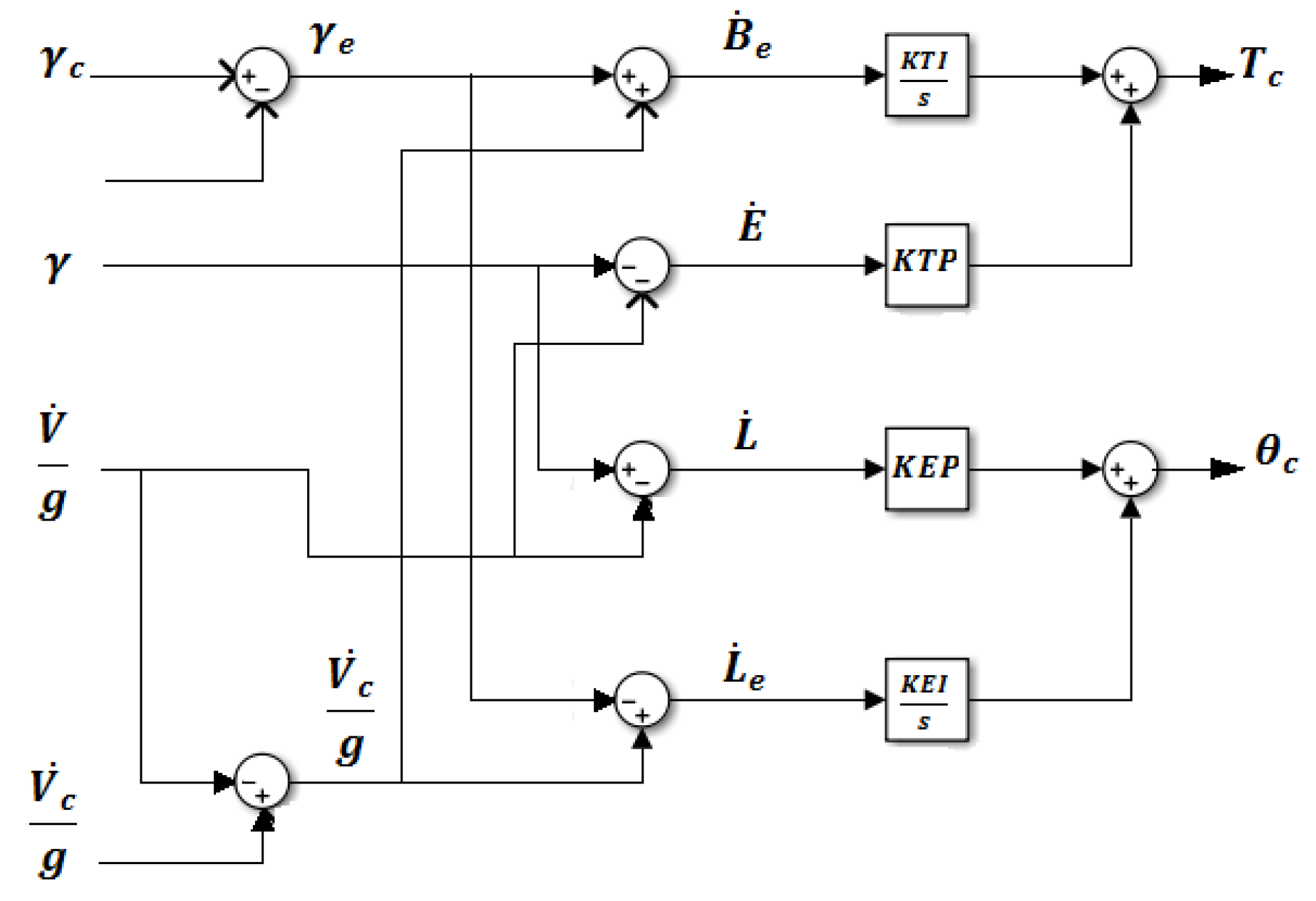
2. Total Energy Control System (TECS)

The aim of TECS design is to calculate the total energy state and desired state of an aircraft. Thrust inputs control the total energy error and elevator inputs control the energy distribution error. Therefore, it is important to derive the energy equations of an aircraft, especially for the total specific energy rate error and the specific energy rate distribution error [11]. Then, the aircraft distribution energy model can be derived from motion and energy equations.

Aircraft Energy Equations

The derivation of energy equations is based on Lambregts [22]. The total energy of an aircraft can be expressed as the sum of the potential energy and kinetic energy, as seen in Equation (3). Assuming constant weight, Equation (3) can be rewritten as:

$$E_T=mg\left({\displaystyle \frac{1}{2}}{\displaystyle \frac{V^2}{g}}+h\right).$$

(4)

Using the small-disturbance theory, the energy of aircraft is linearized at steady flight conditions as:

$$E_{T0}+\Delta E_T=mg\left({\displaystyle \frac{1}{2}}{\displaystyle \frac{{(V_0+\Delta V)}^2}{g}}+(h_0+\Delta h)\right),$$

(5)

where $V_0$ is trimmed airspeed, $E_{T0}$ is the initial total energy, $\Delta E_T$ is the change in the total energy, $\Delta h$ is the change in the flight altitude. Furthermore, it is assumed that the change in the speed $\Delta V^2=0$. Deriving Equation (5) with respect to time:

$${\displaystyle \frac{d}{dt}}(E_{T0}+\Delta E_T)=mg{\displaystyle \frac{d}{dt}}\left[{\displaystyle \frac{1}{2}}\left({\displaystyle \frac{V_0^2}{g}}+{\displaystyle \frac{2V_0\Delta V}{g}}\right)+(h_0+\Delta h)\right],$$

(6)

$$\Delta \dot{E}=mg\left({\displaystyle \frac{V_0\Delta \dot{V}}{g}}+\Delta \dot{h}\right).$$

(7)

Dividing by the trimmed airspeed $V_0$ yields:

$${\displaystyle \frac{\Delta \dot{E}}{V_0}}=mg\left({\displaystyle \frac{\Delta \dot{V}}{g}}+\Delta \gamma \right),$$

(8)

where $\gamma$ is the flight path angle (FPA), which can be expressed in terms of perturbations in pitch attitude $\theta$ and incidence $\alpha$ as follows [23]:

$$\gamma =\theta -\alpha .$$

(9)

Pitch angle is obtained from IMU readings. Both flight and vertical velocity are determined from airspeed sensors to compute the angle of attack. Applying Equation (9), $\gamma$ can be computed. Hence, airspeed value and the rate of change of aircraft energy are dependent only upon the change of longitudinal acceleration, $\Delta \dot{V}$ and the change of flight path angle, $\Delta \gamma$ [22]. Propeller thrust force allows determination of the total energy, which can be derived from the aircraft longitudinal equation of motion, as shown below:

$$m\Delta \dot{V}=\Delta T-\Delta D-mgsin\Delta \gamma ,$$

(10)

where $\Delta D$ is the change in drag force. The aircraft point-mass model is commonly used in energy-based methods [24].

Assuming that $\Delta \gamma$ is small, then $sin\Delta \gamma =\Delta \gamma$; therefore

$$mg\left(\Delta \gamma +{\displaystyle \frac{\Delta \dot{V}}{g}}\right)=\Delta T-\Delta D.$$

(11)

Thus, the aircraft rate of change of energy is proportional to the difference between thrust T and drag D [11]. Rewriting Equation (11), the thrust changes as:

$$\Delta T=mg\left(\Delta \gamma +{\displaystyle \frac{\Delta \dot{V}}{g}}\right)+\Delta D={\displaystyle \frac{\Delta {\dot{E}}_s}{V_0}}mg+\Delta D,$$

(12)

where $\Delta {\dot{E}}_s$ is the total specific energy rate. Assuming that the change in drag force is negligible during the steady flight condition, the change of thrust is proportional to the sum of change of longitudinal acceleration and change of flight path angle [11]:

$$\Delta T\propto \left(\Delta \gamma +{\displaystyle \frac{\Delta \dot{V}}{g}}\right).$$

(13)

Thus, if the drag variation is low, Equations (12) and (13) show that the thrust required is proportional to the specific energy rate of the system. Alternately, it can be stated as the rate at which energy should be delivered to the system. In response to speed or flight path changes, a control law can be developed that uses throttle to drive the total energy rate error to zero [13,25].

$${\delta }_{T_C}=\left(K_{TP}+{\displaystyle \frac{K_{TI}}{s}}\right){\displaystyle \frac{{\dot{E}}_{S_E}}{V}},$$

(14)

where $K_{TP}$ and $K_{TI}$ are the throttle proportional and integral gains, respectively, ${\delta }_{T_C}$ is the change in throttle command, ${\dot{E}}_{S_E}$ is the total specific energy rate error, and s is Laplace operator. Moreover, ${\dot{E}}_{S_E}/V$ is:

$${\displaystyle \frac{{\dot{E}}_{S_E}}{V}}=\gamma +{\displaystyle \frac{{\dot{V}}_E}{g}}.$$

(15)

This control law uses proportional and integral gains to reduce the total energy error to zero with a first-order time constant, $\tau =K_{TP}/K_{TI}$ [22]. Correction of the energy rate distribution error can be done by feeding back the difference of the acceleration error term ${\dot{V}}_E/g$ and the flight path angle error ${\gamma }_E$ [25]. Using proportional plus integral control, the elevator control is:

$${\delta }_{E_C}=\left(K_{EP}+{\displaystyle \frac{K_{EI}}{s}}\right)\left({\displaystyle \frac{{\dot{V}}_E}{g}}-{\gamma }_E\right),$$

(16)

where $K_{EP}$ and $K_{EI}$ are elevator proportional and integral gains respectively, ${\delta }_{E_C}$ is the change in elevator command, and ${\dot{V}}_E$ is the rate of change of airspeed error. Equations (14) and (16) form the TECS core algorithm, as shown in Figure 3, and are based on the natural control behavior of the airplane and its control surfaces.

3. Extended Kalman Filter Description

Another approach would be to use the extended Kalman filter to estimate aircraft attitude. Results are compared with those obtained from the energies-based approach. Assume a nonlinear discrete-time system where $x_k$ is a $m\times 1$ vector, $y_k$ is a $n\times 1$ vector, and $f(x_{k-1},u_k)$ and $g\left(x_k\right)$ are nonlinear functions. This system can be modeled as follows [26]:

$$x_k=f(x_{k-1},u_k)+w_k,$$

(17)

$$y_k=g\left(x_k\right)+v_k.$$

(18)

Equation (17) is called the propagation equation and Equation (18) is called the measurement equation.

3.1. Quaternion-Based EKF

This approach is very important in problems of flight attitude estimation, and has been used by the UAV developers due to its simplicity. The state variables are the unit quaternion (q) and the gyro biases ($b_p$, $b_q$, $b_r$). Besides, measurements of the system are accelerations ($a_x$, $a_y$, $a_z$), and yaw angle ($\psi$) is taken from the magnetometer [27], as shown in Equations (19)–(21):

$$\dot{q}={\displaystyle \frac{1}{2}}\left[\begin{array}{ccccccc}0& -\widehat{p}& -\widehat{q}& -\widehat{r}& 0& 0& 0\\ \widehat{p}& 0& \widehat{r}& -\widehat{q}& 0& 0& 0\\ \widehat{q}& -\widehat{r}& 0& p& 0& 0& 0\\ \widehat{r}& \widehat{q}& -\widehat{p}& 0& 0& 0& 0\\ 0& 0& 0& 0& 0& 0& 0\\ 0& 0& 0& 0& 0& 0& 0\\ 0& 0& 0& 0& 0& 0& 0\end{array}\right]q+w_k,$$

(19)

$$q=\left[\begin{array}{c}{q}_0\\ q_1\\ q_2\\ \underline{q_3}\\ b_p\\ b_q\\ b_r\end{array}\right],\left[\begin{array}{c}\widehat{p}\\ \widehat{q}\\ \widehat{r}\end{array}\right]=\left[\begin{array}{c}p\\ q\\ r\end{array}\right]-\left[\begin{array}{c}{b}_p\\ b_q\\ b_r\end{array}\right],$$

(20)

$$\left[\begin{array}{c}{a}_x\\ a_y\\ a_z\\ \mathsf{\Psi }\end{array}\right]=\left[\begin{array}{c}2g(q_1{q}_3-q_0{q}_2)\\ 2g(q_2{q}_3+q_0{q}_1)\\ g(q_0^2-q_1^2-q_2^2+q_3^2)\\ {tan}^{-1}{\displaystyle \frac{2(q_1{q}_2+q_3{q}_0)}{q_0^2+q_1^2-q_2^2-q_3^2}}\end{array}\right]+{\nu }_k.$$

(21)

3.2. Euler-Angles-Based EKF

Aircraft attitude can be estimated using the following equations where the vector x is the system state (pitch and roll angles) and the vector $\widehat{y}$ is the output (representing accelerometer readings):

$$x=\left[\begin{array}{c}\psi \\ \theta \end{array}\right],\widehat{y}=\left[\begin{array}{c}{a}_x\\ a_y\\ a_z\end{array}\right].$$

(22)

The random variables $w_k$ and $v_k$ represent the process and measurement noise, respectively. They are assumed to be independent. For this study, measurement noise was calculated from the accelerometer accuracy, which is represented using a standard deviation of measured value from true values during the calibration. Process noise and measurement noise covariance matrices in state estimation used for flight tests were selected by having a diagonal matrix in which elements are inversely proportional to sensors’ accuracy. Vectors $\dot{x}$ and $\widehat{y}$ are defined as follows:

$$\dot{x}=\left[\begin{array}{c}p+qsin\varphi tan\theta +rcos\varphi tan\theta \\ qcos\theta -rsin\varphi \end{array}\right]+w_k,$$

(23)

$$\widehat{y}=\left[\begin{array}{c}\dot{u}-rv+qw-gsin\theta \\ \dot{v}+ru-pw-gcos\theta sin\varphi \\ \dot{w}-qu+pv-gcos\theta cos\varphi \end{array}\right]+{\nu }_k.$$

(24)

For small fixed-wing airplanes, where the three axes velocities (u, v, w) are not easily measurable, the air speed ($V_a$) can be used to simplify the measurement equation ($\widehat{y}$). Some assumptions can be made—for example, the aircraft does not change its velocity. So, ($\dot{u}=\dot{v}=\dot{w}=0$), it does not have sideslip velocity ($v=0$), $u=V_{a}cos\theta$, and $w=V_{a}sin\theta$ [27].

$$\widehat{y}=\left[\begin{array}{c}q{V}_{a}sin\theta +gsin\theta \\ r{V}_{a}cos\theta -p{V}_{a}sin\theta -gcos\theta sin\varphi \\ -q{V}_{a}cos\theta -gcos\theta cos\varphi \end{array}\right]+{\nu }_k.$$

(25)

The EKF algorithm estimates 18 states with the equations derived, as follows [9]:

Initial computation (algorithm):

• Navigation EKF controller using a local (north, east, down (NED)) Earth frame;
• XYZ body fixed frame;
• Sequential position and velocity measurements;
• True airspeed;
• Magnetic flux measurement;
• 18-state architecture;
• IMU data;
• IMU angles and velocities are recorded with specified sample time.

State vector:

• Quaternions ($q0$, $q1$, $q2$, $q3$);
• Velocity—m/s (NED);
• Position—m (NED);
• Delta Angles bias—rad;
• Delta Velocities bias—m/s);
• Wind Vector—m/s (NE);
• Earth Magnetic Field—milligauss (NED)
• Body Magnetic Field —milligauss (X,Y,Z).

Observations:

• Velocity—m/s;
• Position—m;
• TAS—m/s;
• XYZ magnetic flux—milligauss;
• XY line of sight angular rate measurements from a downwards-looking optical flow sensor range to terrain measurements.

Time-varying parameters:

• Delta angle measurements in body axes—rad;
• Delta velocity measurements in body axes—m/s.

As shown in the algorithm, angular positions are calculated using angular rates, accelerations are transformed from (X,Y,Z) to Earth NED axes and corrected, while velocity is calculated using accelerations and position is calculated with velocity. Other states are considered, such as gyro biases, vertical acceleration, accelerometer bias, wind vector, compass biases, and the magnetic field. Hence, gyro and accelerometer noise are used to estimate error in calculated angles, velocities, and position. Error can be considerably high if corrections are not made. These estimated errors are captured in the state covariance matrix [9].The extended Kalman filter uses the correlations of errors and states to correct the measured states. In addition, GPS is able to correct errors in velocity, position, gyro bias, and angles.

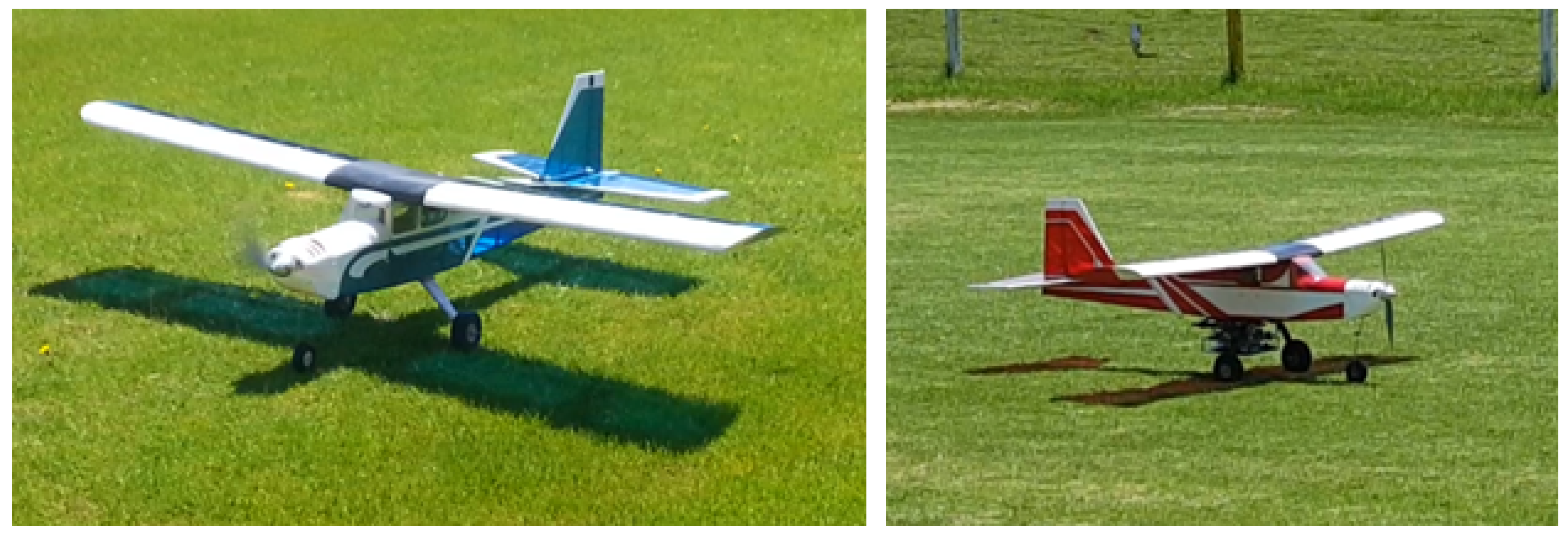
4. Airplane Dynamic Model

To create the equations of motion, it is necessary to consider the UAV as a rigid body and consider the influence of mass and the moment of inertia. Aerodynamic damping effects are also considered, neglecting aeroelasticity effects. Study of the dynamic stability, control, and response of an aircraft implies the consideration of some assumptions established by Bryan [28]. It must be considered that the aerodynamic forces and moments depend only on the instantaneous values of the motion variables in the three aircraft axes. Aerodynamic forces and moments vary linearly with the motion variables. Therefore, the equations are nonlinear and are united in a single set [29]; this is why an analytical solution is difficult to obtain. Therefore, it is assumed that the movement followed after a disturbance is characterized by small amplitudes in all disturbed variables [30]. On the other hand, the aircraft has a vertical plane of symmetry and it is possible to linearize and separate the equations of motion into two groups—longitudinal motion lateral directional motion. For the formulation of the flight dynamics of an aircraft, it is necessary to consider different coordinate systems in such a way that the position, velocity, forces, and moments acting on the aerial vehicle can be specified. The coordinate systems are as follows: inertial axis system, fixed axle system to ground, navigation system, and system of body axes [31].

$$x_{lon}={\left[\begin{array}{cccc}u& w& q& \theta \end{array}\right]}^T,{\dot{x}}_{lon}=A_{lon}{x}_{lon}+B_{lon}{\delta }_{elev}.$$

(26)

First, longitudinal dynamics is decoupled and analyzed taking into account the state equation where:

$$A_{lon}=\left[\begin{array}{cccc}{X}_u& X_w& X_q-W_e& -gcos{\theta }_e\\ Z_u& Z_w& Z_q+U_e& -gsin{\theta }_e\\ M_u& M_w& M_q& 0\\ 0& 0& 1& 0\end{array}\right],B_{lon}=\left[\begin{array}{c}{X}_{{\delta }_{elev}}\\ Z_{{\delta }_{elev}}\\ M_{{\delta }_{elev}}\\ 0\end{array}\right].$$

(27)

Matrices $A_{lon}$ and $B_{lon}$ represent state constants, where $U_e$ and ${\theta }_e$ represent the trim condition. The linearized acceleration measurements are given by:

$$a_x=\dot{u}+q{W}_e+gcos{\theta }_e\theta +gsin{\theta }_e,a_z=\dot{w}-q{U}_e+gsin{\theta }_e\theta -gcos{\theta }_e.$$

(28)

Likewise, lateral direction is coupled between roll and yaw conditions, so the state equation and acceleration are given by:

$$x_{lat}={\left[\begin{array}{ccccc}v& p& r& \varphi & \psi \end{array}\right]}^T,M_{lat}{\dot{x}}_{lat}=A_{lat}^{\prime }{x}_{lat}+B_{lat}^{\prime }\left[\begin{array}{c}{\delta }_{ail}\\ {\delta }_{rud}\end{array}\right],$$

(29)

$$\begin{array}{c}{M}_{lat}=\left[\begin{array}{ccccc}1& 0& 0& 0& 0\\ 0& 1& -I_{xz}/I_{xx}& 0& 0\\ 0& -I_{xz}/I_{zz}& 1& 0& 0\\ 0& 0& 0& 1& 0\\ 0& 0& 0& 0& 1\end{array}\right],A_{lat}^{\prime }=\left[\begin{array}{ccccc}{Y}_v& Y_p-W_e& Y_r-U_e& gcos{\theta }_e& 0\\ L_v& L_p& L_r& 0& 0\\ N_v& N_p& N_r& 0& 0\\ 0& 1& tan{\theta }_e& 0& 0\\ 0& 0& sec{\theta }_e& 0& 0\end{array}\right],\\ B_{lat}^{\prime }=\left[\begin{array}{cc}{Y}_{{\delta }_{ail}}& Y_{{\delta }_{rud}}\\ L_{{\delta }_{ail}}& L_{{\delta }_{rud}}\\ N_{{\delta }_{ail}}& N_{{\delta }_{rud}}\\ 0& 0\\ 0& 0\end{array}\right],\end{array}$$

(30)

$$a_y=\dot{v}-p{W}_e+r{U}_e-gcos{\theta }_e\varphi .$$

(31)

Longitudinal and lateral-directional control and stability derivatives, velocity, and equilibrium terms were obtained using XFLR5. The angular rate stability derivatives were taken from values estimated from gathered flight data. The explicit values of aircraft stability ($A_{lon}$ and $A_{lat}^{\prime }$) and control ($B_{lon}$ and $B_{lat}^{\prime }$) parameters are shown in Equations (32) and (33). They were defined according to [23]. Along with the tested UAV mass, the longitudinal and lateral-directional baseline model is given by:

$$A_{lon}=\left[\begin{array}{cccc}-0.43& 0.65& -0.38& -9.81\\ -0.48& -6.81& 13.32& -0.10\\ 0.19& -7.24& -37.23& 0\\ 0& 0& 1& 0\end{array}\right],B_{lon}=\left[\begin{array}{c}-0.43\\ -3.13\\ -96.32\\ 0\end{array}\right],$$

(32)

$$\begin{array}{c}{M}_{lat}=\left[\begin{array}{ccccc}1& 0& 0& 0& 0\\ 0& 1& -0.143& 0& 0\\ 0& -0.001& 1& 0& 0\\ 0& 0& 0& 1& 0\\ 0& 0& 0& 0& 1\end{array}\right],A_{lat}^{\prime }=\left[\begin{array}{ccccc}-1.35& 0.63& -17.5& 9.81& 0\\ -1.13& -11.41& 23.71& 0& 0\\ 0.33& -0.13& -6.14& 0& 0\\ 0& 1& 0.001& 0& 0\\ 0& 0& 1& 0& 0\end{array}\right],\\ B_{lat}^{\prime }=\left[\begin{array}{cc}0& 5.2\\ -45.1& 17.3\\ -7.01& -16.5\\ 0& 0\\ 0& 0\end{array}\right].\end{array}$$

(33)

Longitudinal and lateral-directional dynamics are computed from an eigenvalue of the system state matrix and presented in

Table 1. Starting point longitudinal lateral-directional dynamics.

Mode	Natural Frequency, rad/s or Time Constant, s	Damping Ratio
Phugoid	0.3671 rad/s	0.6142
Short period subsidence mode 1	0.0297 s	-
Short period subsidence mode 2	0.0963 s	-
Spiral	20.8768 s	-
Dutch roll	4.0796 rad/s	0.9796
Roll	0.0913 s	-

.

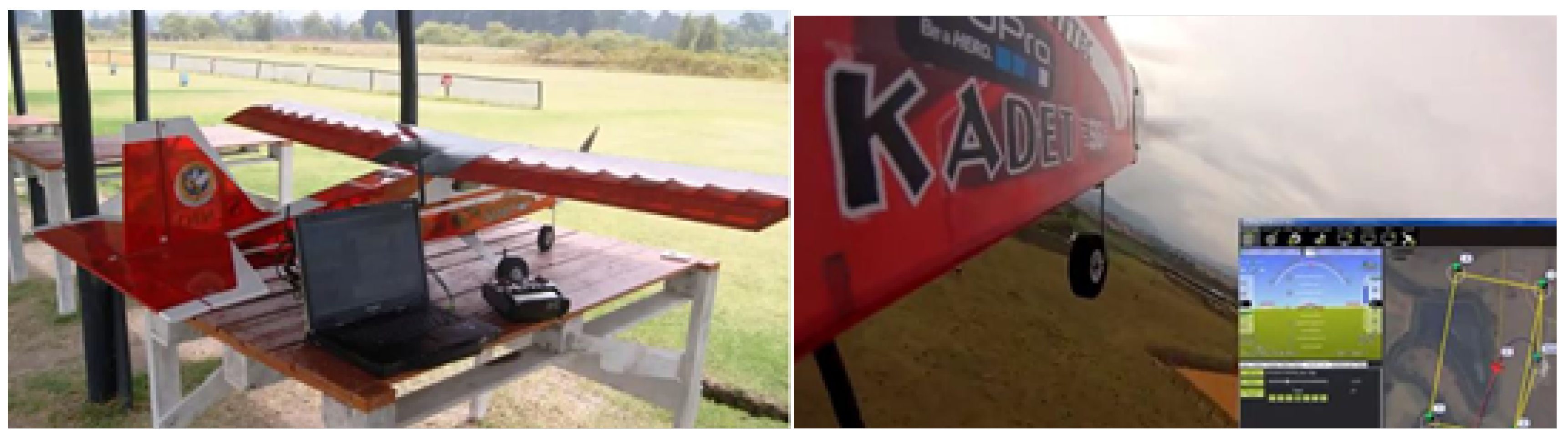
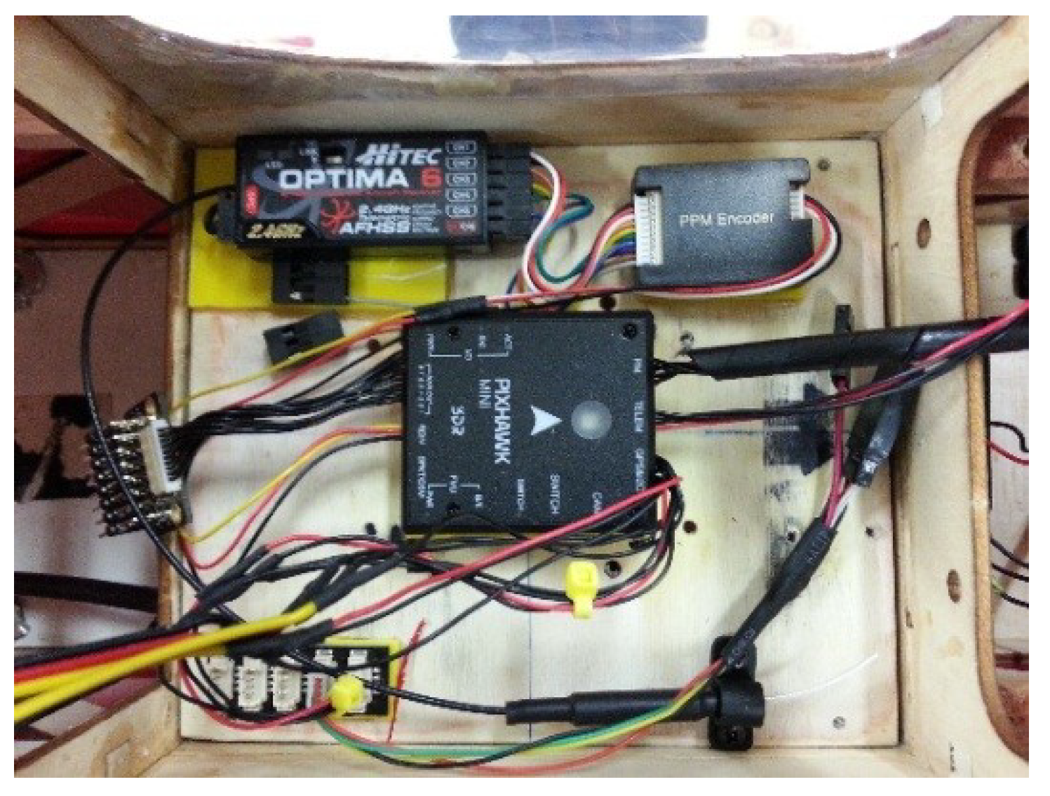
5. Experimental Arrangement

The physical properties of the Kadet Senior UAV system, as well as its hardware and sensor setup are presented in this section. Two test platforms were used to obtain attitude and navigation data, Kadet K1 and Kadet K2, shown in Figure 4. K1 was used to determine pitch, roll, and yaw responses using manual mode to get initial data. K1 is a trainer model that uses an ArduPilot Mega APM 2, which includes one IMU with a barometer, magnetometer, 4 MB dataflash, a GPS uBlox NEO6, a 6 DoF Accelerometer/Gyro MPU-6000 using Atmel’s ATMEGA2560 and ATMEGA32U-2 chips for processing. On the other hand, the K2 UAV was equipped with 3D Robotics Pixhawk autopilot. Both airplanes had a 1300-W brushless motor powered by two 25-V lithium polymer batteries. The payload bay for sensors weighed 800 g to reach a maximum endurance of 15 min at 2600 m above sea level, where flight test were performed. The operation was performed from a ground control station using Mission Planner software, allowing the monitoring of UAV flight data in real time.

K1 and K2 models were 1645 mm long and 2045 mm span, weighed 4950 g (without payload), and had 76.1 dm² of wing area with an average wing load of 65 g/dm². The power systems consisted of one brushless DC electric motor driving a $14\times 7$ in propeller, delivering about 1.4 kg of thrust. Stall speed was 9 m/s and maximum airspeed was 35 m/s.

The K2 UAV Was a conventional fixed-wing airframe with high wing configuration. Two ailerons, one rudder, and one elevator were used as control surfaces. In addition, control surfaces were actuated by Hitec^® electric servos providing a maximum ailerons deflection of 35 deg, maximum rudder deflection of 25 deg, and maximum elevator deflection of 20 deg. The properties of the airframe are shown in

Table 2. Kadet UAV physical properties.

Property	Value	Unit
Mass m	4.95	kg
Wing span b	2.045	m
Mean aerodynamic chord $\overline{c}$	0.38	m
Wing area S	0.76	m2
Moment of inertia $I_{xx}$	0.3175	kg m2
Moment of inertia $I_{yy}$	0.3493	kg m2
Moment of inertia $I_{zz}$	0.5931	kg m2
Moment of inertia $I_{xz}$	0.002593	kg m2

, and the moments of inertia were calculated using XFLR5, as shown in Figure 5 [32].

K2 aircraft was instrumented with a redundant IMU that measured angular rates and translational accelerations. Pixhawk provided actuator commands at 30 Hz, IMU data were recorded at 25 Hz, and the telemetry link sent 3.56 data parameters per second. Flight tests were limited to line-of-sight due to Colombian Civil Aviation Regulations. In addition, the pilot performed takeoff and landing maneuvers. Tests were performed in cruise regime with 60% throttle and 15 m/s desired airspeed.

6. Flight Experiment and Initial Tuning

In this section flight test planning and initial tuning methods are presented to create the conditions for the experimental validation divided into three segments (takeoff, cruise for experiments, and landing) [33]. All conditions are described in cruise and small disturbances for climb, descent, and coordinated turns to validate both EKF and TECS algorithms.

Flight Test

For this case, the study was focused on a typical flight dynamics test pattern [16], whereby the system or process corresponds to each of the flight stages to be evaluated, in order to enhance some analysis or simply to evaluate how far the actual behavior of the aircraft is compared to the predictions obtained from theoretical models. A diagram with the system is shown in Figure 6.

According to Figure 6, prior to designing a flight plan that allows the aircraft dynamic information to be acquired accurately, it is important to determine inputs and outputs from the experiment. In addition, controllable and uncontrollable factors must be considered to determine the possible sources of error that may affect the output variables. The aim of the study was to analyze the critical dynamic parameters during cruise, climb and descent. Thus, variables that needed to be analyzed were selected and a flight plan focused on their measurement was generated in certain periods of time. The experiment airfield was first selected, as described in

Table 3. Experimental location parameters.

Parameter	Value
Airfield location	Bogota, Colombia
Runway altitude	2570 m a.s.l
Runway length	300 m
Runway width	30 m
Latitude/Longitude	4.8240903 deg/−74.1560519 deg
Runway heading	314°–134°

.

During test flights, information related to the variables listed in

Table 4. Parameters measured in-flight.

Parameter	Symbol	Unit
Time	t	s
Relative altitude	h	m
Airspeed	$V_a$	m/s
Ground speed	$V_g$	m/s
Wind speed	$V_w$	m/s
Wind direction	B	deg
Vertical speed	$V_{\nu }$	m/s
Battery remaining	$B_R$	%
Battery voltage	$V_B$	V
Roll angle	$\varphi$	deg
Yaw angle	$psi$	deg
Pitch angle	$\theta$	deg
Roll rate	p	deg/s
Yaw rate	r	deg/s
Pitch rate	q	deg/s
Throttle position	$T_P$	%
Elevator servo	$PWM$	ms

was recorded, filtered, and analyzed to evaluate parameters’ change with respect to time and flight stage.

Mission Planner software was used to create the flight plan from specified waypoints along with some pre-established commands such as loiter, climb, or descend to return to home. Figure 7 shows the proposed flight pattern which was intended to evaluate the aircraft behavior during the climb, cruise, and descent phases. It was proposed to run several repetitions (at least eight) of the pattern for each phase at three different heights, in intervals of 100 m, and to indirectly modify other non-controllable variables such as pressure, temperature, and wind direction.

Experiments were performed in three paths defined at three different heights. Therefore, taking advantage of the variation of heights between each cruise phase, we proposed to evaluate three climbs and three descents for the TECS algorithm. Also, it was defined based on evaluation through a spiral loiter with constant radius, unlike the other two ascents that were made in a straight line for the EKF algorithm. Similarly, for descent, the first two flight lines were set in straight trajectories and the last descent was conditioned to the command Return to Launch (RTL), which must take the aircraft back to 100 m from a height of 300 m to switch to manual mode for landing. On the other hand, the runway selected for tests usually presents winds in the heading of 314 deg. For this reason, a standard heading for all heights was selected for the cruising stages, which was rectangular in shape with 500 m in the direction of 314 deg, to avoid cross-winds during the experiment, and had paths of 350 m perpendicular to the runway to evaluate the parameters under small disturbance conditions caused by lateral winds. The characteristics of the cruise pattern, climb, and descent are detailed in Figure 8.

Flight tests were performed using trainer Kadet K1. Auto-tune mode was then used to setup the aircraft’s initial PID values. Then, the auto-tune level parameter from ArduPilot controller was defined; it controls how the tune is performed. The default level is 6, which produces a medium tune, but we selected level 7, which tunes under faster attitude changes. The manual radio control HiTec Aurora^® was calibrated because it only works for full control movements of pilot sticks. Manual tuning can result in better performance, but it takes more time and effort. Figure 9 shows an example of a 2-min session.

Auto-tune uses a message called ATRP. The first value is for roll tuning, and for pitch tuning, as follows:

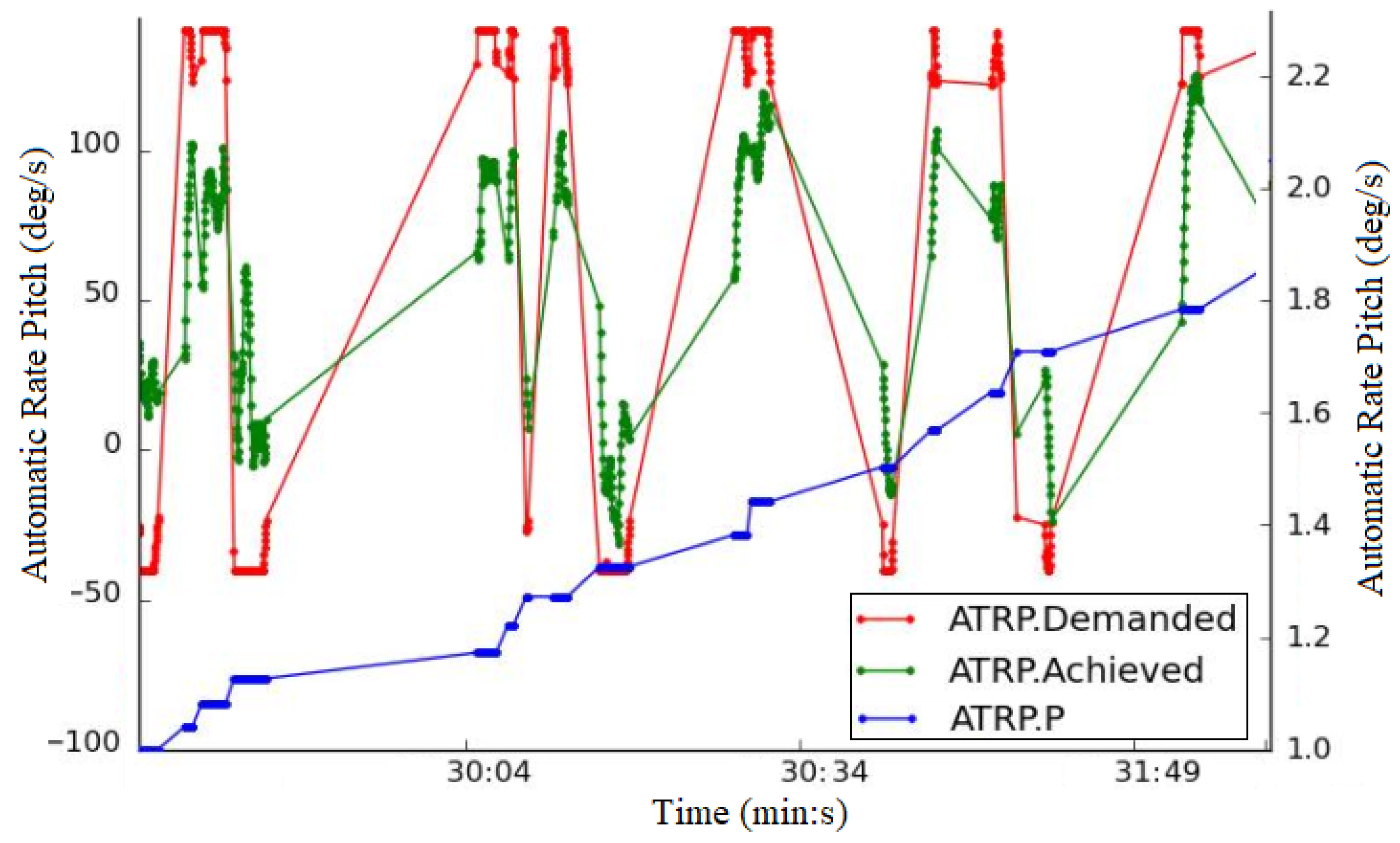
• ATRP.P is the controller P gain.
• ATRP.Achieved is what the aircraft achieved in attitude change rate.
• ATRP.Demanded is the demanded rate of attitude changes (roll rate or pitch rate) deg/s.

It can be seen in Figure 9 that the tune change with the demanded and achieved attitude change started to converge [34,35]. A loop was generated until the airplane responded in the most efficient way.

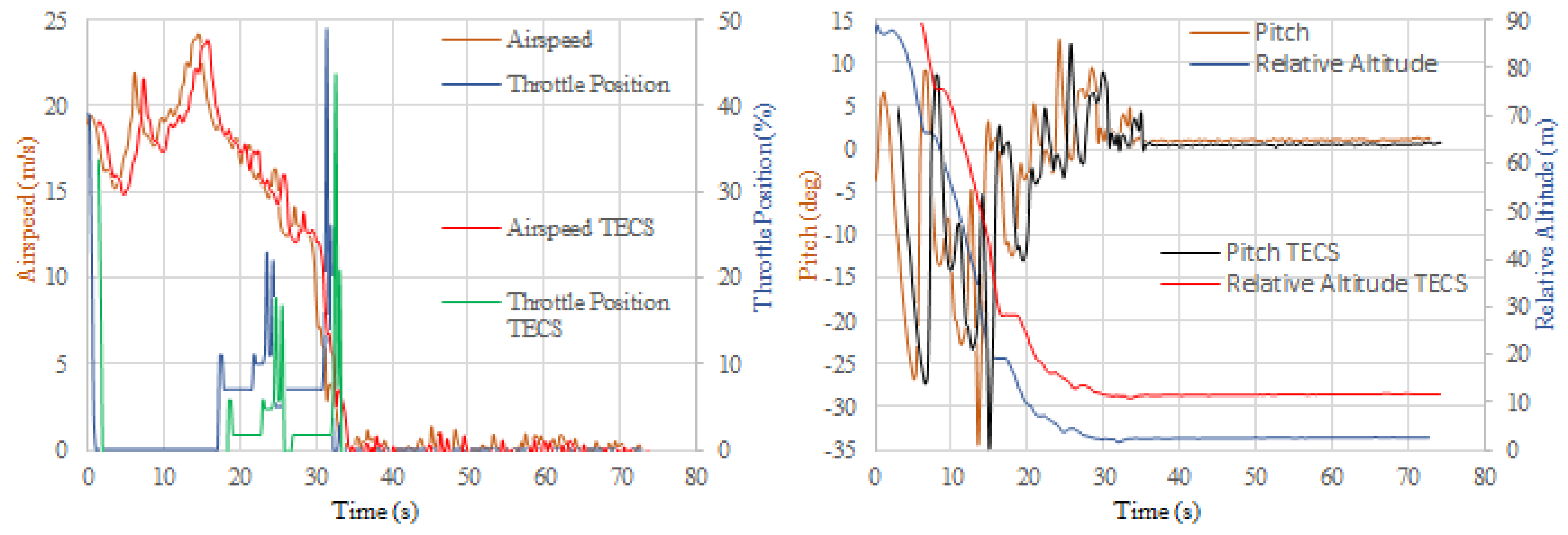
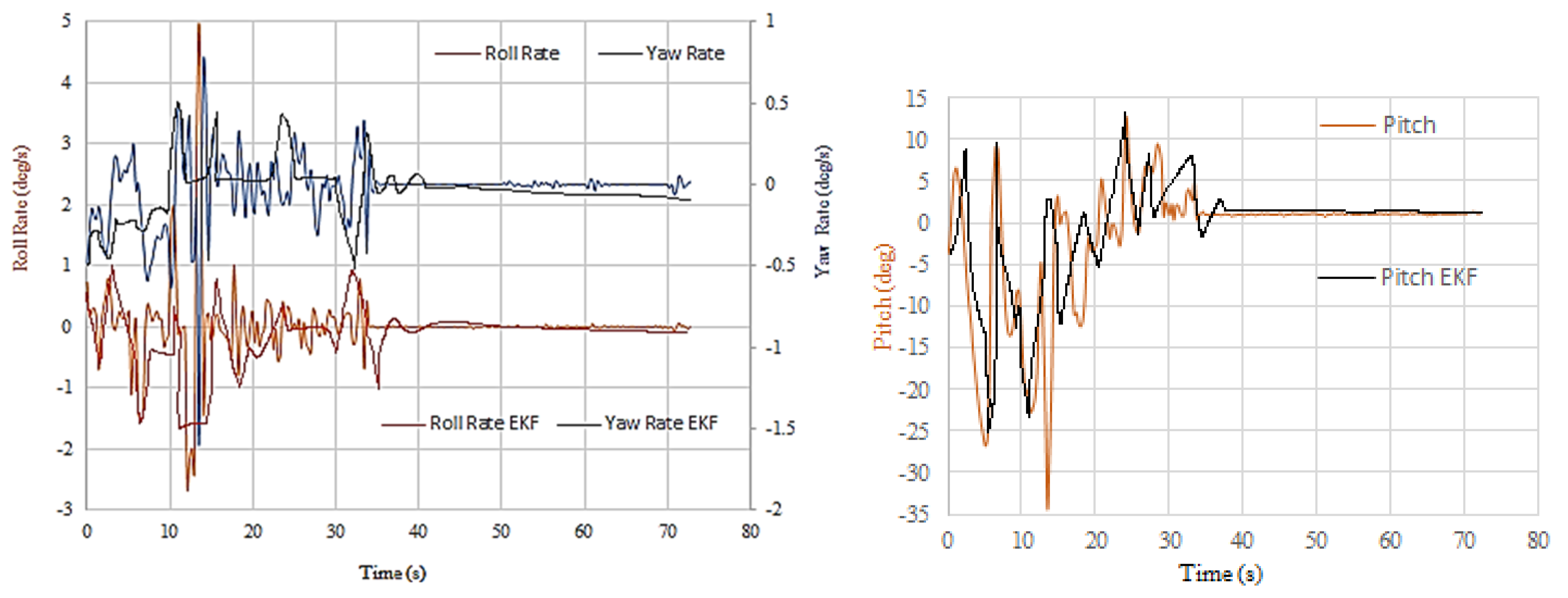
7. Telemetry Analysis and Results

In this section, results validating the theory of TECS and EKF algorithms through flight tests are presented. An 80-s flight path was selected for presentation purposes during different stages of the profile mission. Figure 10 shows TECS validation using airspeed, throttle position, pitch angle, and relative altitude. The TECS algorithm presented a 12.3% pitch, 5.5% airspeed, and 11.1% relative altitude error when compared with the real model. From these results it can be established that algorithm is very accurate and some variables needed to be taken into account to reduce disturbances errors.

On the other hand, the EKF algorithm was validated using equations of motion and system state variables. It was very difficult to make a real estimation due to changes of angular positions and rates due to wind and turbulence disturbances, taken into account and filtered by data extractions.

Figure 11 shows that the model precisely predicted the aircraft’s response. Therefore, the EKF algorithm matched closely; it had an error of 9.5% on average. Besides, the longitudinal and lateral-directional dynamics were decoupled due to elevator responses. The yaw rate response showed discrepancy from the models, due to the use of the L1 controller for navigation between waypoints that are out of range of this research. Regarding the XFLR5 simulation, an average error of 12.3% ws observed between results and flight tests data from the experiment arrangement discussed in Section 6.

Using TECS as a potential and kinetic energy controller is the first step to implement the EKF for applications to estimate vehicle position, velocity, and angular orientation based on rate gyroscopes, accelerometers, compass, GPS, and airspeed and barometric pressure sensors. All these parameters need to be accurately obtained to control and guide unmanned aerial vehicles used in civil and military platforms. Due to TECS and EKF implementation during the flight campaign, the air vehicles were less susceptible to factors that could affect system performance and reliability.

8. Conclusions

A validation using flight tests and theoretical approaches of TECS and EKF algorithms was developed to model the dynamics and control of fixed-wing UAVs. Aircraft dynamics and control were analyzed in the time domain by adjusting nonlinear models to estimate time responses. From the results, it is evident that longitudinal stability increased if the center of gravity was in a forward position, within the allowed ranges. Due to disturbances by wind gusts during the experiment, it was difficult for the aircraft to fly straight and level, which influenced the results, because most of the time it did not maintain the 2 degrees of incidence. However, the reached value was maintained within an acceptable range. Due to air disturbances, the aircraft could not maintain constant height during cruise, but due to the corrections of the elevator it was kept oscillating within a range of 4 m. Because the aircraft took a long time to stabilize during turns, it is recommended to increase the length of the flight pattern for a more effective sampling. The main advantage of this paper is that it shows the successful validation of aircraft dynamics and control using flight data from a single low-cost inertial sensor. Analysis could not be performed in real time because data needed to be downloaded, filtered, and analyzed after each flight. Furthermore, sensors’ sampling frequencies were corrected to compare data at the same frequency. Future studies must be conducted using more accurate IMUs which guarantee same amount of gathered data from each sensor on board. In summary, the procedure can be applied to obtain models that are useful in control applications for aircraft equipped with low-cost sensors.

References

1. Chadli, M.; Maquin, D.; Ragot, J. Vertical Static output feedback for Takagi-Sugeno systems: An LMI approach. In Proceedings of the 10th Mediterranean Conference on Control and Automation, Lisbon, Portugal, 9–13 July 2002. [Google Scholar]
2. Chadli, M.; Borne, P. Multiple Models Approach in Automation- Takagi-Sugeno Fuzzy Systems; John Wiley & Sons: London, UK, 2013; ISBN 978-1-848-21412-5. [Google Scholar]
3. Mohamed, K.; Chadli, M.; Chaabane, M. Unknown Inputs Observer for a Class of Nonlinear Uncertain Systems: An LMI Approach. Int. J. Autom. Comput. 2012, 9, 331–336. [Google Scholar] [CrossRef]
4. Hassani, H.; Zarei, J.; Chadli, M.; Qiu, J. Unknown Input Observer Design for Interval Type-2 T–S Fuzzy Systems with Immeasurable Premise Variables. IEEE Trans. Cybern. 2016, 47, 2639–2650. [Google Scholar] [CrossRef] [PubMed]
5. Eure, K.; Quach, C.; Vazquez, S.; Hogge, E.; Hill, B. An Application of UAV Attitude Estimation Using a Low Cost Inertial Navigation System. NASA Tech. Rep. 2013, 1, 5–7. [Google Scholar]
6. Huang, S. Understanding Extended Kalman Filter. One Dimens. Kalman Filter 2010, 1, 1–9. [Google Scholar]
7. Chao, H.; Coopmans, C.; Di, L.; Chen, Y.U. A Comparative Evaluation of Low-Cost IMUs for Unmanned Autonomous Systems. In Proceedings of the IEEE Conference on Multisensor Fusion and Integration, Salt Lake City, UT, USA, 5–7 September 2010; Volume 1, pp. 2–4. [Google Scholar]
8. Kandath, H.; Pushpangathan, J.V.; Bera, T.; Dhall, S.; Bhat, M.S. Modeling and Closed Loop Flight Testing of a Fixed Wing Micro Air Vehicle. Micromachines 2018, 9, 111. [Google Scholar] [CrossRef] [PubMed] [Green Version]
9. ArduPilot Dev Team. Extended Kalman Filter Navigation Overview and Tuning. Available online: http://ardupilot.org/dev/docs/extended-kalman-filter.html (accessed on 20 December 2019).
10. Qiping, C.; Mulder, B.; Choukroun, D.; Kampen, E.-J.; Visser, C.; Looye, G. Advances in Aerospace Guidance, Navigation and Control; Springer: Berlin/Heidelberg, Germany, 2013; pp. 29–40. ISBN 978-3-642-19817-5. [Google Scholar]
11. Lambregts, A.A. Vertical Flight Path and Speed Control Autopilot Design Using Total Energy Principles. Aiaa Guid. Control. Conf. 1983, 1, 1–5. [Google Scholar]
12. Lambregts, A.A. Total Energy Based Flight Control System. Patent WO 1984001345, 20 August 1984. [Google Scholar]
13. Faleiro, L.F.; Lambregts, A.A. Analysis and tuning of a ’Total Energy Control System’ control law using eigenstructure assignment. Aerosp. Sci. Technol. 1999, 3, 5–9. [Google Scholar] [CrossRef]
14. Kelly, J.; Person, L.; Bruce, K. Flight Testing TECS—The Total Energy Control System. In Proceedings of the SAE Aerospace Technology Conference and Exposition, Long Beach, CA, USA, 13–16 October 1986. [Google Scholar]
15. Brigido-González, J.D.; Rodríguez-Cortés, H. Experimental Validation of an Adaptive Total Energy Control System Strategy for the Longitudinal Dynamics of a Fixed-Wing Aircraft. J. Aerosp. Eng. 2015, 29, 3–8. [Google Scholar] [CrossRef]
16. Jimenez, P.; Agudelo, D.; Cerpa, R.; Zuluaga, E.; Tellez, A. Diseño, análisis y validación de aeronaves no tripuladas multipropósito; Editorial Bonaventuriana: Bogota, Colombia, 2017; pp. 45–75. ISBN 978-958-8928-34-0. [Google Scholar]
17. Balmer, G. Modelling and Control of a Fixed-wing UAV for Landings on Mobile Landing Platforms. Master’s Thesis, KTH Royal Institute of Technology, Stockholm, Sweden, 2015; pp. 60–71. [Google Scholar]
18. Rehan, M.; Tufail, M.; Ahn, C.K.; Chadli, M. Stabilisation of locally Lipschitz non-linear systems under input saturation and quantisation. IET Control. Theory Appl. 2017, 11, 1459–1466. [Google Scholar] [CrossRef]
19. Aouaouda, S.; Chadli, M. Robust fault tolerant controller design for Takagi-Sugeno systems under input saturation. Int. J. Syst. Sci. 2019, 50, 1163–1178. [Google Scholar] [CrossRef]
20. Ferré, J. El diseño factorial completo 2k. Técnicas de Laboratorio 2004, 292, 430–434. [Google Scholar]
21. Jimenez, P.; Agudelo, D. Validation and Calibration of a High-Resolution Sensor in Unmanned Aerial Vehicles for Producing Images in the IR Range Utilizable in Precision Agriculture. In Proceedings of the AIAA SciTech Forum (Infotech @ Aerospace SciTech), Kissimmee, FL, USA, 5–9 January 2015; pp. 734–749. [Google Scholar]
22. Lai, Y.C.; Ting, W. Design and Implementation of an Optimal Energy Control System for Fixed-Wing Unmanned Aerial Vehicles. Appl. Sci. 2016, 6, 369. [Google Scholar] [CrossRef] [Green Version]
23. Cook, M. Flight Dynamics Principles, 3rd ed.; Butterworth-Heinemann: Oxford, UK, 2013. [Google Scholar]
24. Pawełek, A.; Lichota, P.; Dalmau, R.; Prats, X. Fuel-Efficient Trajectories Traffic Synchronization. J. Aircr. 2019, 56, 481–492. [Google Scholar] [CrossRef]
25. Bruce, K.R. NASA B737 Flight Test Results of the Total Energy Control System. In Proceedings of the Astrodynamics Conference, Williamsburg, VA, USA, 18–20 August 1986. [Google Scholar]
26. Welch, G.; Bishop, G. An Introduction to the Kalman Filter; University of North Carolina at Chapel Hill: Chapel Hill, NC, USA, 2006. [Google Scholar]
27. Jang, J.S.; Liccardo, C. Small UAV automation using MEMS. IEEE Aerosp. Electron. Syst. Mag. 2007, 22, 30–34. [Google Scholar] [CrossRef]
28. Bryan, G.; Hartley, G. Stability in aviation: An introduction to dynamical stability as applied to the motions of aeroplanes. Nature 1912, 88, 406–407. [Google Scholar] [CrossRef]
29. Lichota, P. Inclusion of the D-optimality in multisine manoeuvre design for aircraft parameter estimation. J. Theor. Appl. Mech. 2016, 54, 87–98. [Google Scholar] [CrossRef] [Green Version]
30. Agudelo, D.; Lichota, P. A Priori Model Inclusion in the Multisine Maneuver Design. In Proceedings of the 17th IEEE International Carpathian Control Conference (ICCC), Tatranska Lomnica, Slovakia, 29 May–1 June 2016; pp. 440–445. [Google Scholar]
31. Pamadi, B.N. Performance, Stability, Dynamics, and Control of Airplanes; American Institute of Aeronautics and Astronautics: Hampton, VA, USA, 2004; ISBN 978-156-3475-83-2. [Google Scholar]
32. Segui, M.; Kuitche, M.; Botez, R. Longitudinal Aerodynamic Coefficients of Hydra Technologies UAS-S4 from Geometrical Data. In Proceedings of the AIAA Modeling and Simulation Technologies Conference, Grapevine, TX, USA, 9–13 January 2017; pp. 2–4. [Google Scholar] [CrossRef]
33. Dorobantu, A.; Murch, A.; Mettler, B.; Balas, G. System Identification for Small, Low-Cost, Fixed-Wing Unmanned Aircraft. J. Aircr. 2013, 50, 1117–1130. [Google Scholar] [CrossRef]
34. Tucker, A.; Balas, G. Safety, Efficacy, and Efficiency: Design of Experiments in Flight Test. In 56th Annual Society of Experimental Test Pilots Symposium; The Society of Experimental Test Pilots: Lancaster, CA, USA, 2012; pp. 2–10. [Google Scholar]
35. Hartley, R.; Hugon, F.; Anderson, R.; Moncayo, H. Development and Flight Testing of a Model Based Autopilot Library for a Low Cost Unmanned Aerial System. In Proceedings of the AIAA Guidance, Navigation, and Control (GNC) Conference, Boston, MA, USA, 19–22 August 2013; pp. 2–8. [Google Scholar]
Figure 1. (left) SIG Kadet Senior Model Airplane (right) SIG Kadet Senior Model Airplane in flight.
Energies 13 00014 g001
Figure 2. Control system and sensors used in the Kadet Senior UAV.
Energies 13 00014 g002
Figure 3. Total Energy Control System (TECS) core algorithm.
Energies 13 00014 g003
Figure 4. Test platforms (left) K1 (blue) (right) K2 (red).
Energies 13 00014 g004
Figure 5. XFLR5 aerodynamic and stability analysis.
Energies 13 00014 g005
Figure 6. Factors involved during the experiment.
Energies 13 00014 g006
Figure 7. Experimental flight path (left) during ascent (right) during descent.
Energies 13 00014 g007
Figure 8. Top view of cruise pattern.
Energies 13 00014 g008
Figure 9. Kadet K1, auto-tune session example.
Energies 13 00014 g009
Figure 10. TECS validation (left) airspeed and throttle (right) pitch and relative altitude.
Energies 13 00014 g010
Figure 11. EKF validation (left) roll and yaw (right) pitch.
Energies 13 00014 g011