Abstract
Energy, water, and environment are inextricably interwoven in the complex social and economic networks. This study proposes an optimization model for planning the energy–water–environment nexus system (EWENS) through incorporating the linear autoregressive integrated moving average model prediction model (ARIMA), Monte Carlo simulation, chance-constrained programming (CCP), and type-2 fuzzy programming (T2FP) into one general framework. This method effectively tackles type-2 fuzzy set and stochastic uncertainties. The proposed model can quantitatively explore the interconnections between water, energy, and environment systems and generate an optimized solution for EWENS. The proposed model was applied to a coal-dominated region of China, i.e., Inner Mongolia. Several findings and policy implications were obtained. First, the total water supply for energy-generating activities will range from 1368.10 × 106 m3 to 1370.62 × 106 m3, at the end of planning periods. Second, the electricity for water supply will range from 2164.07 × 106 kWh to 2167.65 × 106 kWh at the end of the planning periods, with a growth rate of 46.06–48.72%. Thirdly, lifecycle carbon dioxide emission (LCDE) is projected to range from 931.85 × 10⁶ tons to 947.00 × 10⁶ tons at the end of the planning periods. Wastewater and SO2, NOx, and particulate matter (PM) emissions are projected to be 42.72 × 10³–43.45 × 10³ tons, 183.07 × 10³–186.23 × 10³ tons, 712.38 × 10³–724.73 × 10³ tons, and 38.14 × 10³–38.80 × 10³ tons at the end of the planning periods. Fourthly, as the largest electricity-exporting city of China, Inner Mongolia’s electricity outflows will export 1435.78 × 106 m3 of virtual water to other regions, implying that Inner Mongolia is pumping its important water resource to support other regions’ electricity demands. Finally, high carbon mitigation levels can effectively optimize the electricity power mix, reduce consumption amounts of water and coal, and mitigate air pollutants, wastewater, and LCDE. The obtained results provide useful information for managers to develop a sustainability plan for the EWENS.
1. Introduction
Water, energy, and environment are inextricably interwoven in the complex social and economic networks. Approximately 90% of the energy activities in the world are water-intensive and used for processes such as cooling, steam generation, and desulfurization [1]. Energy is demanded for a series of water-related processes such as surface water extraction, groundwater pumping, water treatment, water distribution, and wastewater treatment [2]. 15% of global withdrawal water is used for energy and 8% of the world’s total energy is used for water [3]. In addition, considerable carbon emissions and pollutants emitted from combustion of fossil fuels for providing water and energy supply, which cause severe environmental pollution and worsen global warming [4]. The environment has become a key factor in maintaining social sustainability [5]. Therefore, it is necessary to incorporate the environment into the analyses of the energy–water nexus, as well as exploring the interconnections between energy, water, and environment systems.
In recent years, many scholars have been devoted to studying the energy markets and the relationships between energy and the economy [6,7,8,9,10,11]. For instance, Tvaronavičienė et al. [6] employed long-range energy-forecasting software LEAP to predict the energy efficiency for selected European countries (Poland, Lithuania, and Germany). Simionescu et al. [7] attempted to analyze the effects of the share in electricity of renewable energy sources and assess the importance of GDP per capita. Their findings indicate a positive but very low impact of GDP per capita on the share in electricity of renewable energy sources in the period of 2007–2017 in the case of the EU countries. Shindina et al. [8] analyzed economic and social properties of the energy market. Their findings show that the interrelationship between heat and electricity acquires a complementary nature, and the rise in prices for one commodity will not necessarily lead to a significant increase in demand for the other. Hnatyshyn [9] employed econometric model to investigate the environmental consequences of economic growth. The results indicate that the relationship between per capita income and emissions of both NH3 and NOx falls into the Environmental Kuznets curve pattern. However, few of these studies considered the interconnections between energy and water and environment systems.
A growing number of studies aimed to study the interconnections between water and energy systems. Input-output model and life cycle analysis have been extensively used to address the energy–water nexus system. For instance, Li et al. [12] adopted the life cycle input-output analysis to analyze the water consumption and CO2 emissions of wind power in China. Feng et al. [13] also used life cycle analysis to provide a detailed account of the water consumption and total LCDE of electricity generation. Nawab et al. [14] developed an extended input-output model to trace Shanghai’s water and energy flows in an economic system from a consumption and production perspective. White et al. [15] employed the input-output model to demonstrate the embodied flows of water, energy, and greenhouse gases in Japan, China, and South Korea via tracing global value chains. Recently, many researchers have analyzed the energy–water nexus based on optimization methods. For instance, Tsolas et al. [3] proposed a systematic method to optimize the energy–water nexus by minimizing the extraction and generation of water and energy resources from the environment and maximizing water and energy yield to meet external demands. Lubega and Farid [16] developed an engineered system model to optimize the coupling points between water and energy systems and thus decrease the energy intensity of water supply and water intensity of energy processing activities. Oke et al. [17] presented a mathematical framework for optimizing the energy–water nexus during shale gas production, processing, distribution, usage, and transmission to maximize overall profit. The majority of these studies focus on evaluating energy consumption for water subsystem, water consumption for energy production and carbon dioxide (CO2) generated from energy–water nexus as well as providing water- and energy-saving suggestions from the perspective of policymaking and technology improvement. However, few of the above studies have taken the environment system into energy–water nexus system. Furthermore, the above studies were based on assumptions that the related parameters such as energy price, operation costs, and electricity demand may be reasonably simplified as deterministic inputs [18]. Few of these studies considered uncertainties, widely existing in energy–water nexus system due to the input parameter measurement, immanent complexity of systems, and subjectivity of human judgment.
Considerable efforts have been made to tackle the uncertainties of traditional energy systems. CCP has been extensively adopted as one method for dealing with random uncertainties. For instance, Wang et al. [19] presented a CCP method to deal with various uncertainties of energy systems and facilitate risk-based management for climate change mitigation. Guan et al. [20] employed CCP method tackle uncertainties in terms of various cost coefficients, and decision maker’s risk attitude which was described by probability distributions. Generally, CCP can tackle the stochastic uncertainties in the right-hand side of constraints and reflect the reliability of satisfying system constraints under uncertainty, but it can hardly determine probabilities of random uncertainties. Monte Carlo simulation is an effective tool for tackling such a problem, which can catch the randomness of available water resources [21,22]. Furthermore, the CCP method is inefficient in addressing the ambiguity and vagueness of subjective judgments. Many economic parameters of are not deterministic and often shown as ambiguity, which are suitably expressed as fuzzy sets [23]. FMP can describe this fuzziness in the energy system [24]. Moradi et al. [25] used an FMP method to deal with the uncertainties regarding energy prices and energy demands to determine the optimum schemes for combined heat and power capacities. Faddel et al. [26] employed an FMP to maximize benefits of aggregators with low charging costs of EV owners, where uncertainties of EV mobility and electricity market were considered. However, A traditional FMP can deal with the ambiguous uncertainties expressed as fuzzy membership functions, but it encounters difficulties when the membership grades of fuzzy uncertainty are also expressed as fuzzy sets (i.e., type-2 fuzzy sets) [27]. As one extension of the conventional FMP, T2FP is more capable of tackling fuzzy uncertainty than conventional fuzzy sets, which is useful in circumstances where it is difficult to determine the exact membership function for a fuzzy set [28].
Although the optimization methods can generate optimized solutions of energy–water nexus system, they may be encounter difficulties when the optimization models need the input data with anticipated prediction accuracy [22]. In particular, the electricity demands, as an important input data of the optimization models, may mislead the optimization results if its prediction accuracy is too low. Multiple linear regression analysis is frequently adopted for forecasting the electricity demands and social economic factors, which is unavailable for reflecting the stochastic and dynamic features of energy–water nexus systems. The ARIMA model is well-known time series prediction method, which emphasizes on analyzing stochastic and probabilistic properties of time series data and has been used for forecasting energy demands [29,30,31]. For instance, Erdogdu [29] used ARIMA model to predict the electricity demand of Turkey. Wang et al. [31] employed ARIMA model to forecast China’s foreign oil dependence.
Summarily, the previous studies mentioned above exists several research gaps that need to be addressed. First, most studies focus on energy–water nexus. However, few of these studies considered the environment system in the energy–water nexus system. Second, several studies were based on the assumption that the related parameter may be reasonably simplified as deterministic inputs, but few of these studies considered the uncertainties that widely exist in energy–water nexus systems. Thirdly, a traditional CCP cannot determine the probability distribution of stochastic parameters, and the traditional FMP encounters difficulties when the uncertainties shown as type-2 fuzzy sets. Fourthly, the previous optimization methods may encounter difficulties when they require high prediction accuracy of the input parameters.
Therefore, this study aimed to make the following contributions: (i) ARIMA model is employed to predict the electricity demands, which is one of the most popular time series models and broadly used for forecasting energy demands [29,30,31]. Monte Carlo is also employed to simulate the probability distribution of electricity demands. The technique makes no assumptions about linear model behavior and it is regarded as a reliable method of uncertainty assessment [32]. (ii) ARIMA–Monte Carlo–chance-constrained–type-2 fuzzy programming method (AM-CT2FPM) is developed through incorporating the ARIMA model, Monte Carlo simulation, CCP, and T2FP into a general framework, which can overcome the shortage of the traditional FMP and CCP methods and tackle type-2 fuzzy sets and stochastic uncertainties. (iii) an AM-CT2FPM-based EWENS (AM-CT2FPM-EWENS) model is proposed by considering environmental factors (i.e., LCDE, particulate matter (PM) nitric oxide (NOX), sulfur dioxide (SO2), emissions and wastewater) in the energy–water nexus. The proposed AM-CT2FPM-EWENS model can quantitatively explore the interconnection between water, energy, and environment systems and generate the optimized solutions of EWENS, including energy production, electricity generation, water for primary energy production (WPEP), water for electricity generation (WEG), electricity for water supply (EWS), and management of LCDE, air pollutants (i.e., NOX, SO2, and PM), and wastewater.
2. Methodology
2.1. ARIMA Model
The ARIMA model is well-known time series prediction method that is originally proposed by Box and Jenkins [33], which emphasizes on analyzing stochastic and probabilistic properties of time series data [29]. The ARIMA model, which has been extensively applied to forecast energy consumption, is used to predict the electricity demands in this study.
The ARIMA model refers to converting a non-stationary time series into a stationary time series and then, regressing only the dependent variable on its lag value, present value, and lag value of the random error term [31]. The autoregressive process (AR) model is the autoregressive model of order p; the moving average process (MA) model is the moving average model of order q; and the ARMA (p, q) is the model with q moving average terms and p autoregressive terms [34]. MA(q), AR(p), and ARMA (p, q) can be applied when the data are stationary. If they are non-stationary, an initial differencing step need to be used to reduce the non-stationarity, namely an ARIMA (p, d, q), where d is the degree of differencing [34]. The AR(p), MA(q) and ARMA (p, q) models are written as follows [35]:
The AR(p) model:
where a1, …, ap are parameters; c is a constant; and the random variable ut is white noise.
yt = c + a1yt−1 + a2yt−2 + … + apyt−p + ut
The MA(q) model:
where θ1, θ2, …, θq are parameters; ut is white noise.
yt = ut + θ1εt−1 + θ2εt−2 + … + θqεt−q
The ARMA (p, q) model:
yt = c + a1yt−1 + a2yt−2 + … + apyt−p + ut + θ1εt−1 + θ2εt−2 + … + θqεt−q
The rules of identifying AR(p), MA(q), and ARMA (p, q) are as follows. The sequence is suitable for the AR model if the partial autocorrelation function (PACF) of the stationary sequence is truncated and the autocorrelation function (ACF) is trailing. The sequence is suitable for the MA model if the PACF of the stationary sequence is trailing and ACF is truncated. The sequence can be concluded to be suitable for the ARMA (p, d, q) model if the PACF and ACF of the stationary sequence are trailing.
In conclusion, ARIMA (p, d, q) model contains four steps: identification, estimation, diagnostic checking, and forecasting [31]. Identification tests the of the sequence smoothness and determines the parameter d. During the second step, the parameters p and q are determined according to the characteristics of ACF and PACF and the models are compared according to the Schwarz’s Bayesian information criterion (BIC) and Akaike’s information criterion (AIC). In the diagnostic checking step, the model based on the results from the previous steps is constructed and estimated and the residuals collected from the previous step are checked to determine whether they are individually statistically significant [29]. Finally, electricity demands are forecasted according to the selected ARIMA (p, d, q) model.
2.2. ARIMA–Monte Carlo–Chance-Constrained–Type-2 Fuzzy Programming Method
Many parameters of EWENS show the characteristics of vagueness because of subjectivity of specialists’ judgment [18,24]. T2FP can effectively cope with ambiguous information in objective and constraint functions, which is useful when the exact membership grade is difficult to determine. T2FP is effective for tackling fuzzy sets with membership grades ranging from 0 to 1 [28]. This characteristic is useful when parameters are highly uncertainty [28,36,37,38]. However, the T2FP method cannot deal with uncertainties expressed as random. In the real-world EWENS, electricity demands, which are closely related to social development and economic growth, may be shown as stochastic variables with probabilistic distribution. CCP can tackle the random uncertainties and analyze the risks of violating constraints [39]. CCP method is especially useful for converting a stochastic programming model into an equivalent deterministic version, and thus significantly reduce system complexities [22]. The detail formulations of T2FP and CCP are put into “Appendix A” section. However, CCP can hardly determine probabilities of random uncertainties. Monte Carlo simulation is an effective tool for tackling such a problem, which can catch the randomness of available water resources.
Therefore, this study aims to propose an AM-CT2FPM through incorporating the ARIMA model, Monte Carlo simulation, CCP, and T2FP into a general framework. An AM-CT2FPM can be formulated as follows:
subject to:
where coefficients , , and are mutually independent type-2 triangular fuzzy numbers defined by , , and ; represents the non-fuzzy decision variable; D, K and R are the deterministic coefficients in the left-hand side of the constraints; is the set with random elements. pi is a given level of probability for constraints (7), which implies that constraint (7) must be satisfied with at least a probability level of 1 − pi. Constraint (7) can be converted into the following constraint: , where , given the cumulative distribution function of Ei, and the probability of violating constraint i. Objective and constraints (5) and (6) can be solved through defuzzification methods [37,38]. α is the credibility levels, indicating the decision maker’s violation risk attitude toward imprecise objective and constraints (5) and (6). A higher α level implies a high likelihood of satisfying fuzzy confidence constraints and less uncertainty regarding imprecise constraints. Different pi and α can directly affect the optimized results of AM-CF2FPM.
The major advantages of AM-CT2FPM include: (i) it is effective for reflecting the stochastic uncertainties in right-hand side constraints, and handling the uncertainties shown as type-2 fuzzy sets in objective and constraints. (ii) It is more capable of dealing with fuzzy uncertainties in real-world applications than the conventional fuzzy sets because type-2 fuzzy set has more design degree of freedom. (iii) It is especially useful for helping the decision makers make their decision based on given probabilities of constraints violations. (iv) It can incorporate other uncertain optimization methods within a general framework.
However, the AM-CT2FPM also has potential limitations should be addressed in future study. First, the AM-CT2FPM can be further improved by combining other uncertainties programming methods (e.g., as interval parameter programming and two-stage programming) into current AM-CT2FPM framework to better address multiple uncertainties and complexities of EWENS. Second, the proposed model aims to minimize system costs with considering a series of constraints of water, energy, and environment systems, which is infeasibility of tackle multi-objectives problems of EWENS. Multi-objective optimization methods for EWENS will be studied in the further research. Figure 1 shows the framework of the proposed AM-CT2FPM.
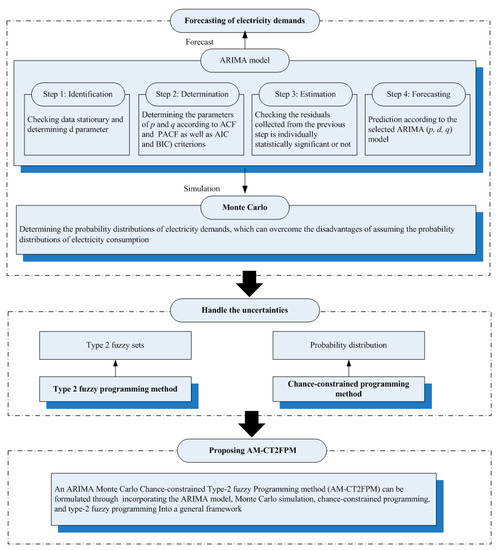
Figure 1.
Framework of the proposed AM-CT2FP.
3. Case Study
3.1. Characteristics of the Study Region
Inner Mongolia Autonomous Region stretches broadly across northern of China, covers 12.28% of the Chinese territory, has 1.82% of Chinese population, and generates 1.93% of the China’s gross domestic product in 2018 [40]. Inner Mongolia is endowed with coal resources (i.e., 51.03 billion tons), which makes it become the China’s largest coal producer. The region’s amounts of coal production were 494.26 million tons of standard coal equivalents (SCE), which accounted for 19.81% of China’s total coal production (2495.16 million tons) in 2017. Crude oil production cannot meet local demand, and the shortage will be imported from other regions. Inner Mongolia has become the largest electricity-exporting city of China. More than 25% of Inner Mongolia’s electricity is exported to other regions such as Liaoning, Hebei, Beijing, and Tianjin. The installed power generation capacity of Inner Mongolia amounted to 118.25 GW, ranking third in China. Coal-based holds a dominant role in the electricity-generation technologies, contributing to 69.09% of the total installed power generation capacity in 2017 [41]. Inner Mongolia is China’s one of the first regions to develop wind power, which has one fifth of total wind power potential [42]. Generation capacity of wind power increased from 8.2 MW in 1995 to 26.7 GW in 2017. Solar power has great development potential in the study region, and its generation capacity was 7.3 GW in 2017. The electricity consumption sharply increased by 136.93% in the past 10 years (from 2008 to 2017) due to rapid social and economic development. Figure 2 presents the information of basic electricity generation, and electricity demands of Inner Mongolia.

Figure 2.
Inner Mongolia’s basic information of energy system.
Inner Mongolia is a typical water-scarce area, and its total water availability amounted to 30.99 billion m3 in 2017 [43]. The water availability per person was 1335.38 m3, which was evidently below the national average of 2069.03 m3 in 2017. The amount of water supply was 18.80 billion m3 in 2017, of which 52.79%, 45.40%, and 1.81% are surface water, groundwater, and recycled water, respectively [43]. The water consumption ratios for household, industry, agriculture, and ecological environment are 5.85%, 8.35%, 73.46%, and 12.29%, respectively. Electricity generation is one of the main water resource consumers in the region, which accounts for approximately 50% of industrial water consumption [43].
Currently, the increasing electricity demands, “high-coal” electric power mix, and expansion of coal-fired power are intensifying the pressure on the environment [44]. CO2 emissions reached to 858.80 million tons, which contributed to 7.40% of China’s national CO2 emissions in 2015 [45]. In 2017, SO2, NOx, and PM emissions, and wastewater reached to 546.25 × 10³ tons, 505.46 × 10³ tons, 536.19 × 10³ tons, and 1042.51 × 106 tons, respectively [40]. Electricity generation is one of the main contributors of LCDE and pollutants in the study region. The increasing frequent occurrences of serious environmental pollution and gravity of global warming have aroused public awareness associated with the mitigation of greenhouse gases and air pollutants as well as improvement of environmental quality.
3.2. Overview of This Study
Energy activities, including primary energy production (crude oil, coal, and natural gas) and electricity generation, are incorporated in the AM-CT2FPM-EWENS model. Multiple energy resources, such as coal, wind, water, and the sun, are supplied to electric power utilities. Four electricity-generation technologies, namely coal-fired power, solar power, wind power, and hydropower, are employed to meet the region’s electricity demands. Most of the generated electricity is distributed to meet local demands. Approximately 30% of Inner Mongolia’s electricity generation would be exported to other regions, and a small portion is used for water subsystem for surface water and recycled water extraction, groundwater pumping, water treatment, water distribution, and wastewater treatment [2]. Groundwater, surface water, and recycled water are supplied to electric power plants for steam generation, cooling, and desulfurization [43]. Many air pollutants, wastewater, and CO2 are emitted from electricity-generation processes.
EWENS is complicated due to the complex relationships between energy subsystem (i.e., primary energy production, electricity generation, and capacity expansion), water subsystem (surface water, groundwater, and recycled water), and environment subsystem (CO2, SO2, NOX, PM, and wastewater) and their interactions with other factors, such as socioeconomic factors, policies, and the ecosystem. In addition, many uncertainties exist in a practical EWENS due to the subjectivity of human judgment, input parameter measurement, and simplifications in model formulation [46]. These uncertainties should be incorporated into the system planning processes. Generally, this study aims to (i) explore the interconnection between energy, water, and environment systems, (ii) employ the developed AM-CT2FPM to tackle the uncertainties of EWENS; and (iii) propose an AM-CT2FPM-EWENS model which can generate optimized solutions for primary energy production, electricity power generation, WPEP, WEG, EWS, and environment management (management of wastewater, LCDE, SO2, NOX, and PM emissions). The study horizon covers a 5-year period (2019–2023), and t = 1 is 2019, t = 2 is 2020, t = 3 is 2021, t = 4 is 2022, and t = 5 is 2023. This study focused on the medium-term planning of Inner Mongolia’s EWENS. Thus, yearly aggregate time data is enough to obtain such a goal. Hourly or daily resolutions will be emphasized in the further research. Figure 3 depicts the framework of the AM-CT2FPM-EWENS model for planning the EWENS.
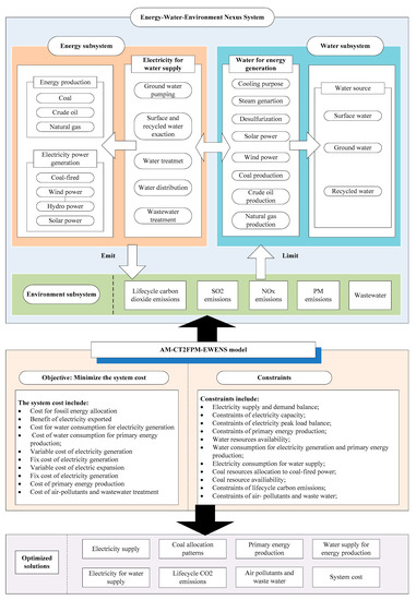
Figure 3.
The framework of AM-CT2FPM-EWENS.
3.3. Modeling Formulation (AM-CT2FPM-EWENS).
Based on the proposed AM-CT2FPM, an AM-CT2FPM-EWENS model was proposed for the sustainability planning of Inner Mongolia’s EWENS. The decision makers can formulate the above problem as to minimize system costs, which include coal resource allocation, electricity importation, water consumption for electricity generation and primary energy production, variable and fixed costs of electricity generation, variable and fixed costs of electric expansion, primary energy production, and pollutant treatment. A series of constraints are considered to be a set of linear equalities or inequalities for defining the relationships of electricity supply and demand; electricity capacity and peak load; primary energy production; water and energy resources availability; WPEP, WEG, and EWS; and LCDE, air pollutant (i.e., NOX, SO2, and PM), and wastewater management. The proposed model is formulated as follows:
Objective:
(1) Cost of fossil energy allocation:
(2) Benefit of electricity exported:
(3) Cost of water consumption for electricity generation:
(4) Cost of water consumption for primary energy production:
(5) Variable cost of electricity generation:
(6) Fix cost of electricity generation:
(7) Variable cost of electric expansion:
(8) Fix cost of electricity generation:
(9) Cost of primary energy production:
(10) Cost of air pollutants and wastewater treatment:
The constraints of AM-CT2FPM-EWENS model are formulated as follows:
- (1)
- Electricity supply and demand balance. Constraints (20) can ensure the total local generated electricity should more than or equal to the sum of local electricity demands and exported electricity. The optimized electricity-generation schemes can be obtained from Equations (21) and (22). The optimized amounts of exported electricity can be obtained from constraints (23) and (24).
- (2)
- Constraints of electricity capacity. Constraints (25) and (26) can guarantee that the capacity of each electricity power technology is greater than the generation amounts of electricity. Constraints (27) and (28) ensure the capacity of each electricity power technology should be greater than its the lower bound and lower than its higher bound.
- (3)
- Constraints of electricity peak load balance. Constraint (30) can guarantee that the electricity load is greater than the electricity peak load of each period.
- (4)
- Constraints of primary energy production. Constraints (31)–(33) require the primary energy lower than their upper limitation.
- (5)
- Water resources availability. The following constraint ensures the water resource consumption for energy activities must be lower than the available water resource amounts for electric power sector and primary energy generation sector.
- (6)
- Water consumption for electricity generation and primary energy production. In detail, the water consumption amounts for each electricity-conversion technology for cooling, steam generation and desulfurization and renewable power can be calculated by the Equations (35)–(38). The water consumption for primary energy production (crude oil, coal, and natural gas) can be obtained by the Equations (39)–(41).
- (7)
- Electricity consumption for water supply. The electricity consumption amounts for surface water supply of electricity generation and primary energy production can be calculated by the Equations (42) and (48); the electricity consumption amounts for groundwater supply of electricity generation and primary energy production can be obtained by the Equations (43) and (49); the electricity consumption amounts for recycled water supply of electricity generation and primary energy production can be calculated by the Equations (44) and (50). For electricity generation and primary energy production, the electricity is required to treat water to meet the standards of energy production. In addition, the electricity consumption amounts for water treatment of electricity generation and primary energy production can be obtained by the Equations (45) and (51). The electricity consumption amounts for water distribution to electricity generation and primary energy production enterprises can be calculated by the Equations (46) and (52). The wastewater treatment is also energy intensive, and it can be calculated by the Equation (47).
- (8)
- Coal resources allocation to coal-fired power. The coal consumption amounts of coal-fired power can be calculated by Equation (53).
- (9)
- Coal resources availability. The constraint ensures the coal resource consumption amounts of coal-fired power must be lower than the total available amounts of coal resources.
- (10)
- Constraints of lifecycle carbon emissions. Equations (56) and (57) are employed for calculating the lifecycle CO2 emissions. Constraint (58) is used for guaranteeing the LCDE should be lower than the carbon emission permit.
- (11)
- Constraints of pollutants (i.e., NOX, SO2, and PM) emissions and wastewater. Equations (59)–(62) are employed for calculating the pollutants. Constraints (63)–(65) are used for meeting the pollutant emissions should be lower than the pollutant permits.
- (12)
- Non-negative constraints. This constraint guarantee decision variables of the proposed model should be always positive.
3.4. Data Collection
Data on annual primary energy production (i.e., crude oil, coal, and natural gas) are obtained from Inner Mongolian Statistical Yearbook 2018 [47]. Data on electricity-installed capacity (i.e., coal-fired, wind, hydro, and solar power), operation hours of electricity-conversion technology, and electricity demands are mainly collected from Editorial committee of the China Electric Power Yearbook 2018 [41]. Electricity demands are often expressed as stochastic information; the ARIMA model was used for predicting Inner Mongolia’s electricity demands and Monte Carlo simulation is employed to catch the randomness of the characteristic of electricity demands. Data regarding water supply and local water availability are retrieved from the Water Resources Bulletin 2017 [43]. Water intensity factors for coal, crude oil, and natural gas production are 0.35 m3/tce, 0.762 m3/tce, and 0.42 m3/tce, respectively [48]. Water intensity factors for cooling, stream generation, desulfurization, wind power, hydropower, and solar power were 1.17 m3/MW, 0.27 m3/MW, 0.08 m3/MW, 0.00 m3/MW, 13.00 m3/MW, and 0.03 m3/MW, respectively [46,48]. Energy intensity factors of water supply were obtained from [49]. Depending on different water sources, energy intensities for surface water, recycled water extraction, and groundwater pumping are 0.95 kWh/m3, 0.82 kWh/m3, and 0.31 kWh/m3, respectively. Electricity is required for water treatment, and the energy intensity of water treatment is 0.414 kWh/m3. The energy intensity for water distribution is 0.495 kWh/m3. At the last step of EWENS cycle, wastewater collection and treatment also need energy, and its energy intensity is 0.50 kWh/m3 [48]. The LCDE factors of coal-fired power, wind power, and solar power are 1213.50 g/kWh, 34.40 g/kWh, and 67.40 g/kWh [42]. The LCDE factor of hydropower is 35.535 g/kWh [13]. The emissions factors of SO2, NOx, PM, and wastewater are 5.20 g/kWh, 1.14 g/kWh, 6.00 g/kWh, and 60 g/kWh, respectively [41]. Due to the inherent uncertainties and complexities of the EWENS, many economic parameters are provided as type-2 fuzzy sets, which are shown in Appendix B [44].
4. Result Analysis
Numerous results can be obtained from the AM-CT2FPM-EWENS model. Four electricity-generation technologies, three primary energy production types, LCDE, four pollutants, and five periods have been considered in the AM-CT2FPM-EWENS model. Furthermore, four carbon mitigation levels, six p levels, and three α levels were calculated using the proposed model. Therefore, p = 0.01 and α = 0.9 were selected to depict the results and related policy implication generated from the AM-CT2FPM-EWENS model. To compare the impacts of carbon reduction on EWENS, different carbon mitigation levels (μ = 0.0%, μ = 0.5%, μ = 1.0%, and μ = 1.6%) are considered in this study. The upper limit of CO2 reduction of EWENS was 1.6% according to the results generated from the AM-CT2FPM-EWENS model.
4.1. Electricity Demand Prediction
The ARIMA model was employed to predict Inner Mongolia’s electricity demands in periods 1–5. Electricity demand (E) data are annual data from 1995 to 2018, which were collected from the National Bureau of Statistics. The data are converted into natural logarithms (Log E). According to the rules of identifying ARIMA (p, d, q), ARIMA (2, 1, 4) with AR = 2, d = 1 and MA = 4 is chosen as the best ARIMA model to forecast the electricity demands of Inner Mongolia. Results of the ARIMA (2, 1, 4) model are achieved using EViews 9 software [29]. As results, the electricity demand will show an increased trend over the planning periods, with a growth rate of 55.73%. In detail, it will be 356.02 × 10⁹ kWh, 378.88 × 10⁹ kWh, 441.332 × 10⁹ kWh, 510.71 × 10⁹ kWh, and 554.44 × 10⁹ kWh in periods 1, 2, 3, 4, and 5, respectively. This is attribute to the increasing electricity demands as the societal and economic rapidly development of Inner Mongolia region. The detail results of ARIMA (p, d, q) are provided in Appendix C.
Monte Carlo simulation was employed to generate the probability distribution of electricity demand. According to the results of electricity demand through ten thousand times of Monte Carlo runs in periods 1–5, the normal distribution was the best fitting performance for the distribution of random variables. The prediction value generated by the ARIMA model would be the mean values of electricity demand, and the standard deviations value would be 2 billion kWh for each period. Figure 4 shows the probability distributions of electricity demand in periods 1–5, which would be used as the inputs of the AM-CT2FPM-EWPNS model.

Figure 4.
The probability distribution of electricity demand.
4.2. Electricity Supply
Figure 5 presents the optimized pattern for electricity generation under different μ levels during the study periods. The major power conversion technologies of Inner Mongolia include coal-fired, wind, hydro, and solar power. Several major regularities are indicated in Figure 5. First, the electricity-generation amounts will be 911.38–911.43 × 10⁹ kWh at the end of the planning periods, which is expected to increase by 54.97–54.99% due to the rapid social and economic development. This is attribute to the rapidly development of societal and economic of Inner Mongolia region. Second, coal-fired power holds the primary role in the study region, which constitutes from 77.34% to 85.14% over the planning periods. This condition is mainly because Inner Mongolia is rich in coal resources, serving as a safeguard for energy security of China. As a result, Inner Mongolia has become the largest electricity-exporting region of China. A total of 26.38% of Inner Mongolia’s generated electricity would be exported to other regions. The exported electricity is projected to be 155.09 × 10⁹ kWh in period 1, 164.94 × 10⁹ kWh in period 2, 191.77 × 10⁹ kWh in period 3, 221.61 × 10⁹ kWh in period 4, and 240.42 × 10⁹ kWh in period 5, respectively. Third, renewable energy is expected to undertake enormous development space given that the Chinese government has devoted to promoting renewable power under a series of policies such as the 13th Five-Year Plan and Paris Agreement. There is a huge potential for the study region to develop wind power and wind power will play an increasingly significant role owing to its abundance. The electricity generated by wind power will be 105.12 × 10⁹ kWh in period 1, 107.07 × 10⁹ kWh in period 2, 109.01 × 10⁹ kWh in period 3, 110.32 × 10⁹ kWh in period 4, and 111.35 × 10⁹ kWh in period 5, respectively. The results also indicate that the electricity generated by wind power will be not affected by the μ-cut levels. Solar power is expected to increase by approximately 22.15–29.84% over the planning periods. Hydropower will make up a minor share of total electricity power generation and keep steady (i.e., 3.09 × 10⁹ kWh) across the planning periods in Inner Mongolia due to water resource shortage of the study region. Hydropower contributes only 0.34–0.52% of the total power generation by the end of the study periods. Lastly, high carbon mitigation levels can accelerate the area’s electric power mix shift from coal-dominated to low-carbon pattern. As a result, the coal-fired power will show a decreasing trend with enhancement in the μ-cut level. For example, in period 1, the electricity generated from coal-fired power will be 462.70 × 10⁹ kWh when u = 0.0%, 460.23 × 10⁹ kWh when u = 0.5%, 457.76 × 10⁹ kWh when u = 1.0%, and 454.80 × 10⁹ kWh when 1.6%. In addition, solar power would be 17.20 × 10⁹ kWh when u = 0.0%, 19.66 × 10⁹ kWh when u = 0.5%, 22.12 × 10⁹ kWh when u = 1.0%, and 25.07 × 10⁹ kWh when 1.6%. Therefore, additional policies associated with “stricter carbon emission mitigation” should be proposed to optimize the region’s electric power structure.
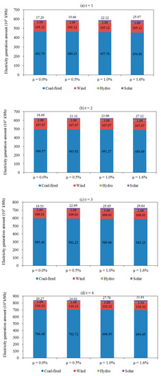
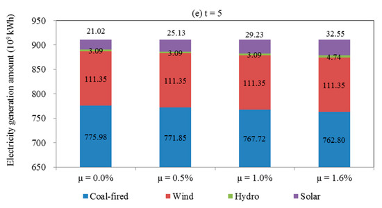
Figure 5.
Optimized solutions of electricity supply.
4.3. Water Supply for Energy Production
Table 1 shows the water resource supply for electricity generation and primary energy production under different μ levels across the study horizon. Several findings are indicated in Table 1. First, the total water supply for energy activities (i.e., WPEP and WEG) in Inner Mongolia will show an increased trend over the planning periods. The total water supply for energy activities is expected to range from 922.04 × 10⁶ m3 to 933.80 × 10⁶ m3 in period 1 under different μ levels. The obtained results are similar to Chu et al. [48]. The results of Chu et al. [48] indicate the water consumption for energy production is 934.00 × 10⁶ m3. In addition, it will increase to 1368.10 × 106 m3–1370.62 × 106 m3 at the end of the planning horizon under different μ levels, with a growth rate of 46.51–48.65%. This finding is mainly attributed to the increasing electricity demands and strong water dependency of power generation in Inner Mongolia. Approximately 79.26–85.86% of water consumption will be associated with electricity generation, whereas 14.14–20.74% was associated with primary energy production. Surface water and groundwater contribute 52.79%, 45.40% of the total water supply, whereas recycled water contributes 1.81%. This is quite different from the situation of Xiamen, where the shares of surface water and recycled water are 65% and [26.0, 33.9]% according to the results of Liu et al. [50].

Table 1.
Water input for electricity generation and primary energy production.
Second, coal-fired power consumes the most water resources of all power generation technologies, which accounts for 94.41–96.69% of WEG over the planning horizon. Most water is consumed for cooling purposes because evaporative cooling system is the dominant cooling technology in the study region. For example, the water input for cooling purpose is expected to account for 72.77–76.17% of total WEG amounts under different μ levels. This finding indicates that switching from evaporative cooling to air cooling system can effectively mitigate water stress in Inner Mongolia. On the contrary, steam generation and desulfurization are projected to consume only 15.68–16.47% and 4.29–5.20% of total WEG amounts, respectively.
Thirdly, the water consumption for renewable power should not be neglected as hydro and solar power also require water inputs to generate electricity. The water input of hydropower remained stable and will be 40.11 × 10⁶ m3 across the planning periods. The water consumption of solar power is expected to increase by 14.61–21.83% under different μ levels over the planning horizon. The results also indicate that it is particularly important to the study region to reap the benefit of lower water consumption by switching from traditional coal-based to low-carbon electricity-generation mix. The results of this study also indicate that wind power is project to potentially save 149.59 × 10⁶ m3 of water resource.
Lastly, high carbon mitigation levels are helpful to close the gap of water shortage in water-scarce regions. The study region could be switched from a coal-dominated to “low-carbon” mix area, which cannot only save fossil fuels but also significantly decrease water consumption of electricity generation. As a result, a 1% increase in carbon mitigation level (from 0.0% to 1.0%) is projected to reduce water input by 7.35 × 10⁶ m3, 7.74 × 10⁶ m3, 9.10 × 10⁶ m3, 10.79 × 10⁶ m3, and 11.84 × 10⁶ m3 in periods 1–5, respectively.
Figure 6 presents the virtual water contributed by electricity outflows. The results indicate an alarming situation that Inner Mongolia is projected to experience water stress across the planning periods. As Figure 6, as the largest electricity-exporting city of China, exporting virtual water via coal-fired power is expected to increase from 235.27 × 10⁶ m3 in period 1 to 351.22 × 10⁶ m3 in period 5 (based on the assumption that the exported electricity is generated by coal-fired power). Chu et al. [48] indicates that the virtual water outflow of Inner Mongolia will range from 150 × 106 to 300 × 106 m3 in 2014, which is similar to the results of this study. The results imply that Inner Mongolia, as a water-scarce area, is pumping its precious water resource to support other region’s electricity demands. Such a situation raises concerns on the adjustment of the current energy pattern in China.

Figure 6.
Virtual water contributed by electricity outflows.
4.4. Electricity Consumption for Water Supply
Several findings of EWS are presented in Table 2. First, EWS will range from 2164.07 × 106 kWh to 2167.65 × 106 kWh at the end of the planning periods, with a growth rate of 46.06–48.72%. The amount of EWS is projected to contribute approximately to 0.4% of the study region’s total electricity demands. Second, the water-sourcing phase is expected to account for 41.54–41.57% of the total EWS amounts, of which 76.32% and 21.42% of electricity use will be associated with surface water extraction and groundwater pumping, whereas recycled water provided 2.26% of water supply. The electricity for water treatment and water distribution ranges between 26.17–26.19% and 31.29–31.31%, respectively. Wastewater treatment constitutes 0.93–0.99% of total EWS amounts. The portion is extremely low compared with other developed cities (i.e., Beijing, Shanghai and Xiamen) [48,50]. Lastly, high carbon mitigation requirement can significantly reduce the amounts of WEG and EWS. As a result, a 1% increase in carbon mitigation level would decrease electricity by 11.66 × 10⁶ kWh, 12.28 × 10⁶ kWh, 14.43 × 10⁶ kWh, 17.11 × 10⁶ kWh, and 18.78 × 10⁶ kWh in periods 1–5, respectively.
Table 2.
Electricity allocation patterns for water supply.
4.5. Lifecycle Carbon Dioxide Emissions of EWENS
Several inferences can be withdrawn from Figure 7, which shows the LCDE generated from electricity-generation process over the planning horizon. First, the total LCDE will show an increased trend over the planning periods, which is projected to range from 557.31 × 10⁶ to 566.38 × 10⁶ tons in period 1. In addition, it will increase to 931.85 × 10⁶ tons–947.00 × 10⁶ tons at the end of the planning horizon under different μ levels, which is more than the LCDE of German in 2017 [51]. LCDE is expected to increase by 67.20% over the planning horizon due to the increasing electricity demands. Li et al. [42] estimated that coal-fired power would contribute to 1.3 billion tons of CO2 emissions in Inner Mongolia by 2020, which is significantly higher than the results of this study. This is mainly because the study of Li et al. [42] might overestimate the power generation capacity of coal-fired power (i.e., 240.0 GW), which apparently higher than the results of this study (102.08 GW) and the historic data of 81.70 in 2017 [41].

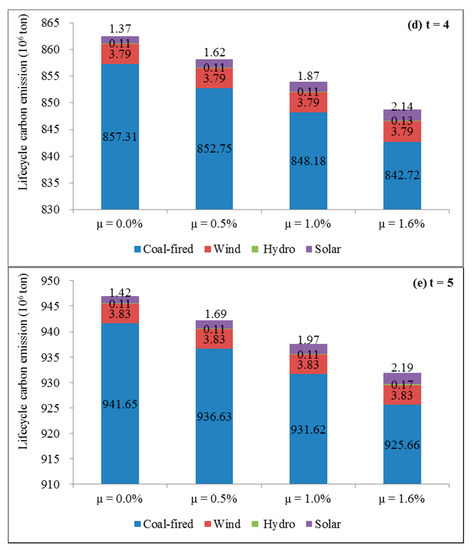
Figure 7.
Lifecycle carbon dioxide emissions.
Second, sources of LCDE vary substantially across different types of electricity-conversion technologies. Coal-fired power will be major contributor for LCDE in the study region, and it emits more than 99% of total LCDE in the region. The high emissions of coal-fired power generation are mainly due to the large emissions from mining, combustion of fossil fuel, and operation of power plants. Renewable electricity-conversion technologies have much lower LCDE and indirect emissions from upstream processes compared with coal-fired power generation. The LCDE for wind power is projected to increase from 3.62 × 10⁶ tons in period 1 to 3.83 × 10⁶ tons in period 5. The results also show that the development of wind power is project to potentially reduce 118.55 × 10⁶ tons of LCDE. Hydropower would contribute only 0.11 × 10⁶ tons of total LCDE in each period because it will remain stable and contribute a minor share over the planning periods. The LCDE of solar power is expected to increase by 22.15–32.17% over the planning horizon under different μ levels. The significant differences in LCDE between different electricity-conversion technologies indicate that substantial mitigation in CO2 emissions can be achieved by substituting the existing coal-dominated power mix with a low-carbon pattern.
Thirdly, the results indicate that EWS will only contribute a small fraction of total LCDE. This amount will be 2626.10 × 103–2630.45 × 103 tons at the end of the planning horizon under different μ levels, with a growth rate of 46.60–48.72%. Lastly, high carbon mitigation requirement can effectively optimize the electric power mix and save coal resources, reducing the amounts of LCDE. Results indicate that a 1% increase in carbon mitigation level (from 0.0% to 1.0%) is projected to decrease LCDE by 5.66 × 10⁶ tons, 6.08 × 10⁶ tons, 7.28 × 10³ tons, 8.63 × 10³ tons, and 9.47 × 10³ tons in periods 1–5, respectively.
Figure 8 shows the LCDE contributed by electricity outflows. As the largest electricity-exporting region of China, the electricity outflows of Inner Mongolia are expected to contribute 188.20 × 10⁶ tons of LCDE in period 1 (as Table 2). This amount will increase to 291.74 × 10⁶ tons at the end of the planning horizon, which is similar to the LCDE of Poland in 2015 [51]. This result is lower than that of Li et al. [42] (520 million ton). This is because Li et al. [42] overestimated the power generation capacity of coal-fired power (i.e., 240.0 GW) and the domestic electricity outflows of the total power generation amounts (40%) in Inner Mongolia by 2020, which is higher than the historical data [41,47] and the result of this study.

Figure 8.
Lifecycle carbon dioxide emissions contributed by electricity outflows.
4.6. Pollutants Emissions of EWENS
Wastewater, NOx, SO2, and PM are selected as the pollutants that managers aim to mitigate because of their harmful impacts on the environment and human health. Several inferences can be drawn from Figure 9, which displays the pollutants from electricity-generation process across the study horizon under different μ levels. First, results indicate an uptrend of pollutants from period 1 to period 5. Wastewater, SO2, NOx, and PM are projected to be 42.72 × 10³–43.45 × 10³ tons, 183.07 × 10³–186.23 × 10³ tons, 712.38 × 10³–724.73 × 10³ tons, and 38.14 × 10³–38.80 × 10³ tons at the end of the planning periods under different μ levels, with a growth rate of 56.52–56.54%, 54.80–54.82%, 54.29–54.30%, and 39.77–39.75%, respectively. This finding is attributed to the increasing trend of electricity-generation amounts and electricity demands.

Figure 9.
Pollutants emitted from electricity generation.
Second, EWS would contribute a small fraction of pollutants. For example, when μ = 0.0%, the wastewater, SO2, NOx, and PM will be 121.19 × 10³–121.39 × 10³ tons, 519.38–520.24 tons, 497.74–498.56 tons, and 108.20–108.38 tons in period 5 under different μ levels, with a growth rate of 36.83–38.81%, 35.32–37.28%, 34.87–36.83%, and 21.17–23.94%, respectively, over the planning periods.
Lastly, high carbon mitigation requirement could effectively optimize the electric power mix and save coal resources, leading to lower pollutants. Results indicate that a 1% increase (from 0.0% to 1.0%) in carbon mitigation level is projected to decrease 1.87 × 10⁶ tons, 8.05 × 10³ tons, 7.73 × 10³ tons, and 1.76 × 10³ tons of wastewater and SO2, NOx, and PM emissions, respectively, over the planning horizon.
Table 3 shows the virtual environment pollutants contributed by electricity outflows. The pollutants contributed by exporting electricity are projected to show an increasing trend. Wastewater, SO2, NOx, and PM emitted by electricity outflows are expected to be 13.46 × 10⁶ tons, 57.70 × 10³ tons, 55.30 × 10³ tons, and 12.02 × 10³ tons, respectively, in period 5, with a growth rate of 44.69%, 43.10%, 42.62%, and 29.18%, respectively, across the planning horizon.
Table 3.
The virtual environment pollutants contributed by electricity outflows (103).
4.7. Coal Allocation Patterns for Electricity Generation and Primary Energy Production
Figure 10 presents the coal consumption amounts of coal-fired power across the planning horizon under different μ levels. Several findings are presented in Figure 10. First, the coal consumption amounts of coal-fired power are expected to be 231.89 × 10⁶–235.90 × 10⁶ tons of SCE at the end of the planning periods, with a growth rate of 63.40–63.42%. This increase is mainly attributed to the increasing electricity demands and coal-dominated power generation of Inner Mongolia. Thus, a large amount of coal is consumed as fuel for power generation.

Figure 10.
Coal consumption amounts of coal-fired power.
Second, as the largest electricity-exporting city of China, 26.38% of Inner Mongolia’s electricity-generation amounts would be exported to other regions. This situation indicates that electricity outflows will consume 48.39 × 10⁶ tons of SCE, 51.13 × 10⁶ tons of SCE, 59.06 × 10⁶ tons of SCE, 67.81 × 10⁶ tons of SCE, and 73.09 × 10⁶ tons of SCE of coal resource in periods 1–5, respectively, based on the assumption that the exported electricity are generated by the coal-fired power.
Thirdly, high carbon mitigation levels can effectively save coal resources. A 1% increase in carbon mitigation level (from 0.0% to 1.0%) is projected to save 1.54 × 10⁶ tons of SCE, 1.64 × 10⁶ tons of SCE, 1.96 × 10⁶ tons of SCE, 2.30 × 10⁶ tons of SCE, 2.51 × 10⁶ tons of SCE coal resource in periods 1–5, respectively. This finding is mainly because high μ levels can promote the city’s electric power system shift from being coal-dominated to a diversified electricity power mix, which will save the coal inputs of coal-fired power.
Figure 11 presents several results of the optimized solutions of primary energy production across the study periods. First, the coal production amounts will show a steady increasing trend over the planning horizon. It is expected to be 501 × 106 tons of SCE at the end of the planning periods, with a growth rate of 2.10%. Inner Mongolia was defined as an energy-dependent and energy-output-oriented region as more than half of its coal resources would be exported to other provinces. Second, the production amounts of natural gas will be stable across the planning periods. More than 80% of the natural gas resource is projected to be exported to other provinces. Third, the production amounts of crude oil are expected to show a decreasing trend across the planning periods. Local crude oil production amount cannot meet the local demands, of which more than 80% will be compensated by importing from other provinces.

Figure 11.
Optimized solutions of primary energy production.
4.8. System Cost
Figure 12 shows the system costs across the study horizon under different μ levels. As can be observed from Figure 12, the fixed and variable cost of electricity generation, cost of coal allocation, and primary energy production cost are projected to contribute largely to the system cost. Their shares will be 36.88–38.82%, 24.39–25.84%, 13.09–14.02%, and 11.79–12.41%, respectively. A system benefit of RMB ¥499.00 × 10⁹ will be achieved through exporting electricity to other regions. Furthermore, Figure 12 also shows that the system costs are expected to increase with raised μ levels. For instance, the system costs will be RMB ¥4891.39 × 1012, 4969.05 × 1012, 5046.71 × 1012, and 5148.84 × 1012 under μ values of 0.0%, 0.5%, 1.0%, and 1.6%, respectively. Results also indicate that a 1% increase in carbon mitigation level (from 0.0% to 1.0%) is projected to increase system cost by RMB ¥155.32 × 10⁹. This finding is because a high μ level can accelerate the renewable power development and increase the costs corresponding to electric expansion of renewable power.

Figure 12.
System costs under different μ levels.
5. Discussion
Six p levels (i.e., 0.01, 0.05, 0.10, 0.15, 0.20, and 0.30) and three different credibility levels (i.e., 0.8, 0.9, and 1.0) are considered to understand the influences of the uncertainties on the optimized solutions of EWENS. The planning problem of EWENS can also be solved through conventional CCP by neglecting the fuzzy uncertainties. This study compares the optimized solutions of EWENS generated from AM-CT2FPM with that from CCP method.
5.1. Uncertainties Analysis
Table 4 shows the optimized solutions for EWENS under different p levels over the planning periods. Six p levels of violating electricity demand (i.e., 0.01, 0.05, 0.10, 0.15, 0.20, and 0.30) on the electricity demands are considered, which corresponded to various reliabilities of meeting the region’s electric power system demands. For example, p = 0.01 implies that electricity demands must be satisfied at the probability of (1 − 0.01 = 0.99). The results indicate that the amounts of electricity supply will decrease as the p levels increase. For instance, the electricity supply will decrease from 4440.93 × 109 kWh (p = 0.01) to 4405.53 × 109 kWh (p = 0.30). This is mainly because decision with high p level corresponds to a high risk of violating the region’s electricity demands, and thus a lower electricity demand. Suo et al. [28] aimed to plan the Shanghai’s energy system with CCP method, which obtained the similar trend with this study. They found that the electricity supply amount would decrease from 665.3 × 10³ GWh under p = 0.01 to 657.7 × 10³ GWh under p = 0.20. Variations in the p level correspond to the decision makers’ preferences regarding the tradeoff between electricity supply and risk of violating the electricity demand constraint. Pessimistic managers will prefer to lower p levels, which can guarantee the electricity demands be met, leading to high electricity supply amounts. Contrarily, Optimistic managers tend to choose higher p levels, resulting in relaxed electricity demand constraints and lower electricity supply amounts.
Table 4.
Optimized solutions under different p levels over the planning horizon.
Furthermore, high electricity supply amounts will lead to high WEG, EWS, LCDE, air pollutant, and wastewater. Thus, WEG, EWS, LCDE, air pollutant, and wastewater have similar trends with the electricity supply amounts. Decision with high p level leads to a reduced strictness for the electricity demand constraint and thus decreased amounts of WEG, EWS, LCDE, air pollutants, and wastewater. Contrarily, decisions with a low p level associate with a low risk of violating the electricity demands but result in high amounts of electricity supply, WEG, EWS, LCDE, air pollutants, and wastewater. Results also shows that the system cost will decrease with the raised p levels. Liu et al. [50] used CCP model to plan energy–water nexus system of Xiamen, which found that the system cost would increase form RMB¥ [456.29, 732.52] × 109 (with p = 0.05) to RMB¥ [416.56, 673.73] × 109 (with p = 0.10). Yu et al. [52] used CCP model to plan municipal energy system with considering peak-electricity price, which shown that a higher p level of peak-electricity demand would lead to a lower system cost and decrease reliability in fulfilling the electricity demands. The relationships between system cost and p levels reported by Liu et al. [50] and Yu et al. [52] were consistent with this study. Summarily, p levels can reflect the manager’s preferences regarding the tradeoff between system failure and system cost. Pessimistic manager prefers to a low p level which can meet the electricity demands and thus lead to higher system costs. Optimistic manager tends to a high p level which leads to low electricity supply and system costs but increases the risk of electricity shortage. Managers should choose between a riskier solution with a higher p level and more conservative scheme with a lower p level.
Table 5 presents the optimized solutions of EWENS under different credibility levels α of 0.8, 0.9, and 1.0. The credibility levels α indicate the decision maker’s attitude of violation risk toward imprecise constraints. A high α levels imply high likelihoods of satisfying fuzzy confidence constraints and less uncertainty regarding imprecise constraints. The imprecise objective and constraints of and can be converted into a conventional linear programming model though using the proposed method. Several inferences can be drawn from Table 5. First, according to type-2 fuzzy theory, a high credibility level will lead to an increment value in terms of and decrement coefficient in terms of . This finding indicates that a high credibility level α has advantages in accelerating the shift of electricity mix from being coal-dominated to a low-carbon mix pattern. For example, the electricity generated from coal-fired power will be reduced by 532.22 × 10⁶ kWh and electricity generated from solar power is expected to increase by 488.61 × 10⁶ kWh when the credibility levels α increase from 0.8 to 1.0. Second, the tendency of LCDE, wastewater, and air-pollutant emissions will be similar to the electricity generated by coal-fired power because it is expected as the major contributor of electricity in Inner Mongolia. Third, a high credibility level will correspond to high WEG and EWS due to the evident development of solar power and hydropower. Lastly, the system costs are expected to increase with increased credibility levels α. This finding is mainly because a high α level implies high coal prices and operation costs of electric power as well as great amounts of electricity generated from renewable power. This phenomenon leads to increased costs corresponding to WEG, EWS, and renewable power expansion and operation. Kundu et al. [37] aimed to reduce the type-2 fuzzy variable into type-1 fuzzy variables and employed the type-2 fuzzy method to solve the transportation problems. They found that a higher α levels will correspond to higher transportation costs. For instance, the transportation costs will decrease from 239.50 (α = 0.9) to 227.04 (α = 0.7). The results of Kundu et al. [37] are similar to this study. Generally, a high credibility degree can increase the strictness of the constraints but results in a high system cost. On the contrary, a low credibility degree corresponds to an aggressive attitude of decision makers on the system costs, leading to a high uncertainty of imprecise constraints.
Table 5.
Optimized solutions under different credibility levels (α) over the planning horizon.
5.2. Comparison with CCP
The problem of EWENS for Inner Mongolia can be converted into a conventional CCP problem by simplifying the membership grades of type-2 fuzzy sets into crisp values. Table 6 presents the optimized solutions generated from the AM-CT2FPM and CCP method over the planning horizon (μ = 1.6%; p = 0.05, and α = 0.9). Several inferences can be drawn from Table 6. First, the results indicate that an AM-CT2FPM can effectively support the transformation of electric power mix from a coal-dominated pattern to a low-carbon pattern. For instance, electricity generated by coal-fired power under the AM-CT2FPM will be lower than that under CCP, and electricity generated from solar power under AM-CT2FPM will be higher than that from CCP. Second, WEG and EWS under AM-CT2FPM will slightly higher than those under CCP, mainly because AM-CT2FPM can obviously accelerate the development of renewable power. Third, LCDE, wastewater, and air pollutants from AM-CT2FPM will be lower than those from CCP, which indicates that AM-CT2FPM has an advantage in reducing LCDE, wastewater, and air pollutants compared with CCP. Fourth, the AM-CT2FPM model will lead to a higher system cost, mainly because the economic parameters tackled by AM-CT2FPM are higher than those tackled by CCP. The results show that AM-CT2FPM is more capable of decreasing dependence on coal-fired power and reducing LCDE, wastewater, and air pollutants for the study area, but lead to a higher system cost. Generally, AM-CT2FPM is more advanced in optimizing EWENS and tackling the uncertainties.
Table 6.
Optimized solutions under AM-CTFPM and CCP over the planning horizon.
6. Conclusions
In this study, an AM-CT2FPM is developed through incorporating the ARIMA model, Monte Carlo simulation, CCP, and T2FP into one general framework, which is capable of effectively tackling the uncertainties shown as type-2 fuzzy sets and stochastic. The proposed model can overcome the shortage of traditional FMP and CCP methods; the ARIMA model is used to predict the electricity demands; and Monte Carlo is employed to simulate the probability distribution of electricity demands. Based on the AM-CT2FPM, an AM-CT2FPM-EWENS model is proposed by considering the environment sector (i.e., SO2, NOX, PM, and wastewater) in the energy–water nexus. This method can quantitatively explore the interconnections between water, energy, and environment systems and generate optimized schemes for EWENS, including electricity power generation, primary energy production, WPEP, WEG, EWS, and management of LCDE, air-pollutant emissions, and wastewater.
The proposed model was applied to Inner Mongolia, a coal-dominated region of China. Several findings were obtained, which can provide a scientific basis for planning EWENS:
- (1)
- The total water supply for electricity generation and primary energy production in Inner Mongolia will range from 1368.10 × 106 m3 to 1370.62 × 106 m3 at the end of the planning horizon under different μ levels, with a growth rate of 46.51–48.65% across the planning horizon. In detail, 79.26–85.86% and 14.14–20.74% of water consumption would be due to electricity generation and primary energy production, respectively.
- (2)
- The EWS will range from 2164.07 × 106 kWh to 2167.65 × 106 kWh at the end of the planning periods, with a growth rate of 46.06–48.72%. The water-sourcing phase, water treatment, water distribution, and wastewater treatment are expected to account for 41.54–41.57%, 26.17–26.19%, 31.29–31.31%, and 0.93–0.99% of total EWS amounts, respectively.
- (3)
- The lifecycle carbon dioxide emissions will range from 931.85 × 10⁶ tons to 947.00 × 10⁶ tons at the end of the planning horizon, which will increase by 67.20% over the planning horizon. Wastewater and SO2, NOx, and PM emissions are projected to be 42.72 × 10³–43.45 × 10³ tons, 183.07 × 10³–186.23 × 10³ tons, 712.38 × 10³–724.73 × 10³ tons, and 38.14 × 10³–38.80 × 10³ tons at the end of the planning periods under different μ levels, with a growth rate of 56.52–56.54%, 54.80–54.82%, 54.29–54.30%, and 39.77–39.75%, respectively.
- (4)
- Inner Mongolia has become the largest electricity-exporting city of China. Approximately 26.38% of Inner Mongolia’s electricity-generation amounts would be exported to other regions. That indicating electricity outflows will consume 299.48 × 10⁶ tons of SCE of coal resource, export 1435.78 × 106 m3 of virtual water to other region, and contribute 1181.73 × 106 tons, 242.32 × 10³ tons, 232.58 × 10³ tons, 52.99 × 10³ tons, and 56.25 × 10⁶ tons of LCDE, SO2, NOx, PM, and wastewater across the planning horizon. The results imply that Inner Mongolia, as a water-scarce area, is pumping its precious water resource to support other region’s electricity demands.
- (5)
- High carbon mitigation levels can effectively optimize the electricity power mix, reduce consumption amounts of water and coal, and mitigate air pollutants, wastewater, and LCDE. However, a high system cost is incurred in the process. A 1% increase in carbon mitigation level is projected to reduce 9.95 × 10⁶ tons of SCE, 46.82 × 10⁶ m3, 37.11 × 10³ tons, 1.87 × 10⁶ tons, 8.05 × 10³ tons emission, 7.73 × 10³ tons, and 1.76 × 10³ tons of coal resource, water resource, LCDE, wastewater, and SO2, NOx, and PM emissions, respectively, over the planning horizon. However, the system cost will significantly increase by RMB ¥155.32 × 10⁹ over the study horizon.
The results indicate that AM-CT2FPM can effectively lessen dependence on coal-fired power, save water resource, and reduce LCDE, wastewater, and air pollutants for the study area compared with conventional CCP method. To understand the influences of the uncertainties on the optimized solutions of EWENS, different p levels (i.e., 0.01, 0.05, 0.10, 0.15, 0.20, and 0.30) and three different credibility levels (i.e., 0.8, 0.9, and 1.0) are considered in this study. The results indicate that the system cost will decrease with the raised p levels, which is consistent with the results of Liu et al. [50] and Yu et al. [52]. In addition, the system costs are expected to increase with increased credibility levels α, which is similar to the study of Kundu et al. [37]. The results generated from the AM-CT2FPM-EWENS model can support local policymakers in developing a sustainability plan for EWENS. The proposed model can be extended to other regions in the world. However, the proposed model aims to minimize system costs with considering a series of constraints of water, energy, and environment systems, which is infeasibility of tackle multi-objectives problems of EWENS. Multi-objective optimization methods for EWENS will be studied in the further research.
Author Contributions
C.C. proposed and calculated the AM-CT2FPM-EWENS model, as well as written the manuscript; L.Y. made contributions to the Monte Carlo simulation and prediction of electricity demands; X.Z. collected the data, analyzed related data; G.H. contributed in conceptualization of idea; Y.L. contributed in editing the manuscript. All authors have read and agreed to the published version of the manuscript.
Funding
This research was supported by the national natural science fund projects (No. 41701621, 71673022). Beijing Municipal Social Science Foundation (No. 18LJC006, 17LJB004). The national natural science fund projects (No. 71704010). The authors are grateful to the editors and the anonymous reviewers for their insightful comments and suggestions.
Conflicts of Interest
The authors declare no conflict of interest.
Abbreviations
| System costs; | |
| Cost of fossil energy allocation; | |
| Benefit of electricity exportation; | |
| Cost of water consumption for electricity generation; | |
| Cost of water consumption for primary energy production; | |
| Variable cost of electricity generation; | |
| Fix cost of electricity generation; | |
| Variable cost of electric expansion; | |
| Fix cost of electric generation; | |
| Cost of primary energy production; | |
| Cost of air pollutants and wastewater treatment; | |
| Type of electric power, = 1, 2, 3, 4; = 1 for coal-fired power, = 2 for wind power, = 3 for hydro power, and = 4 for solar power; | |
| Study periods, = 1, 2, 3, 4, 5; t = 1 is 2019, t = 2 is 2020, t = 3 is 2021, t = 4 is 2022, and t = 5 is 2023. | |
| pi | A give level of probability for constraint n, implying that the constraints n should be satisfied with at least a probability level of 1 − pi. |
| α | The confidence levels; |
| Model Parameters | |
| The price of coal resources; | |
| The price of electricity exported; | |
| The loss rate of electricity transmission; | |
| The cost of water for cooling; | |
| The cost of water for steam generation; | |
| The cost of water for desulfurization; | |
| The cost of water resource to renewable power; | |
| The cooling water consumption of unit of electricity power generation; | |
| The boiler water consumption of unit of electricity power generation; | |
| The desulfurization water consumption of unit of electricity power generation; | |
| The water consumption amounts of unit of renewable power; | |
| The water consumption intensity of coal production; | |
| The water consumption intensity of crude oil production; | |
| The water consumption intensity of natural gas production; | |
| The cost of water resource for coal production; | |
| The cost of water resource for crude oil production; | |
| The cost of water resource for natural gas production; | |
| The cost of operation cost of first-stage electricity power generation; | |
| Fixed-charge cost of capacity expansion for electricity power conversion technology; | |
| Residual capacity of each electricity power conversion technology; | |
| The production cost for coal resource; | |
| The production cost for coal resource; | |
| The production cost for coal resource; | |
| The cost for desulfurization; | |
| The cost for denitration; | |
| The cost for PM removal; | |
| The cost for wastewater treatment; | |
| The desulfurization efficiency; | |
| The denitration efficiency; | |
| The PM removal efficiency; | |
| The electricity demands under various pi levels, which shown the characteristic of stochastic; | |
| The lower bound of exported electricity; | |
| The upper bound of exported electricity; | |
| The operating hours of electricity-conversion technology; | |
| The residual capacity for each electric power technology; | |
| The upper bound for capacity expansion of each electric power technology; | |
| The upper load demands of capacity of each electric power technology; | |
| The electricity peak load demand; | |
| The upper bounds for coal resource production; | |
| The lower bounds for coal resource production; | |
| The upper bounds for crude oil resource production; | |
| The lower bounds for crude oil resource production; | |
| The upper bounds for natural gas resource production; | |
| The lower bounds for natural gas resource production; | |
| The amounts of available water resource for electricity generation and primary energy production; | |
| Electricity intensity factors for surface water supply; | |
| Electricity intensity factors for ground water supply; | |
| Electricity intensity factors for recycled water supply; | |
| Electricity intensity factors for water treatment; | |
| Electricity intensity factors for water distribution; | |
| Electricity intensity factors for wastewater treatment; | |
| The proportion of surface water in total water resources supply; | |
| The proportion of ground water in total water resources supply; | |
| The proportion of recycled water in total water resources supply; | |
| Coal consumption intensity factor for coal-fired power; | |
| The amounts of available coal resource for coal-fired power generation; | |
| The life cycle CO2 emissions coefficient; | |
| The SO2 emission coefficient; | |
| The NOX emission coefficient; | |
| The NOX emission coefficient; | |
| The wastewater emissions coefficient; | |
| The total allowance amounts of life cycle CO2 emissions; | |
| The total allowance amounts of SO2 emissions; | |
| The total allowance amounts of NOX emissions; | |
| The total allowance amounts of PM emissions; | |
| Decision Variables | |
| The electricity-generation amounts of each electricity-conversion technology; | |
| The electricity generated from the capacity expansion for each electric power; | |
| The optimized electricity-generation schemes of each electricity-conversion technology; | |
| The electricity consumption amounts for surface water supply of electricity generation; | |
| The electricity consumption amounts for ground water supply of electricity generation; | |
| The electricity consumption amounts for recycled water supply of electricity generation; | |
| The electricity consumption amounts for water treatment of electricity generation; | |
| The electricity consumption amounts for water distribution to electricity-generation enterprise; | |
| The electricity consumption amounts for wastewater treatment of electricity generation; | |
| The electricity consumption amounts for surface water supply of primary energy production (i.e., coal, crude oil, and natural gas); | |
| The electricity consumption amounts for groundwater supply of primary energy production (i.e., coal, crude oil, and natural gas); | |
| The electricity consumption amounts for recycled water supply of primary energy production (i.e., coal, crude oil, and natural gas); | |
| The electricity consumption amounts for water treatment of primary energy production (i.e., coal, crude oil, and natural gas); | |
| The electricity consumption amounts for water distribution to primary energy production enterprise (i.e., coal, crude oil, and natural gas); | |
| The amounts of exported electricity; | |
| Continuous variable of electric capacity expansion of each electricity power type; | |
| The total water consumption amounts for coal production; | |
| The total water consumption amounts for crude oil production; | |
| The total water consumption amounts for natural gas production; | |
| The total cooling water consumption amounts for each electricity power type; | |
| The total boiler water consumption amounts for each electricity power type; | |
| The total desulfurization water consumption amounts for each electricity power type; | |
| The total water consumption amounts for each renewable power; | |
| The coal consumption amounts of coal-fired power; | |
| The life cycle CO2 emission amounts; | |
| The SO2 emission amounts; | |
| The NOx emission amounts; | |
| The PM emission amounts; | |
| The wastewater emission amounts; | |
| The production amounts for coal resource; | |
| The production amounts for crude oil resource; | |
| The production amounts for natural gas resource; | |
Appendix A. The Detailed Formulation of T2FP and CCP
Appendix A.1. Type-2 Fuzzy Programming
Many parameters of EWENS show the characteristics of vagueness because of subjectivity of specialists’ judgment [18]. T2FP is effective for tackling fuzzy sets with membership grades ranging from 0 to 1. This characteristic is useful when parameters are highly uncertainty [21]. A type-2 fuzzy set in X is a fuzzy set and its membership function is also expressed as fuzzy set. is represented as [36]:
where is the type-2 membership function, is the primary membership of , which is the domain of the secondary membership function so that all are primary membership grades of point x [37].
A type-2 triangular fuzzy variable (TFV) is defined as , where can characterize the degree of uncertainty that takes a value x. A type-2 TFV is deemed as an extension of type-1 TFV. For a type-1 TFV (r1, r2, r3), the range of the membership grade is fixed values (from 0 to 1). However, for a type-2 TFV , the primary memberships of the points are no longer fixed values but range between 0 and 1. θl and θr denote the spreads of primary possibilities of type-2 TFV. Type-2 TFV becomes a type-1 TFV when θl = θr [37]. The secondary possibility distribution function of is represented by [38]:
A type-2 fuzzy set is more capable of dealing with fuzzy uncertainties in real-world applications than the conventional fuzzy sets, because type-2 fuzzy set has more design degree of freedom [21]. A T2FP model can be formulated as follows [37]:
subject to:
where coefficients , , and are mutually independent type-2 triangular fuzzy numbers defined by , , and ; represents the non-fuzzy decision variable. D and K are the deterministic coefficients in the left-hand side of the constraints.
Qin et al. [38] developed a critical value (CV)-based reduction method which can reduce a type-2 fuzzy variable to a type-1 fuzzy variable. According to Kundu et al. [37], the model Formulations (A3)–(A6) can be converted into the following crisp equivalent parametric programming problems:
- (i)
- When the generalized credibility level , the model Formulations (A3)–(A6) are equivalent to:subject to:
- (ii)
- When the generalized credibility level , the model Formulations (A3)–(A6) are equivalent to:subject to:
- (iii)
- When the generalized credibility level , the model Formulations (A3)–(A6) are equivalent to:subject to:
- (iv)
- When the generalized credibility level , the model Formulations (A3)–(A6) are equivalent to:subject to:
T2FP can effectively cope with ambiguous information in objective and constraint functions, which is useful when the exact membership grade is difficult to determine. However, the T2FP method cannot deal with uncertainties expressed as random. In the real-world EWENS, electricity demands, which are closely related to social development and economic growth, may be shown as stochastic variables with probabilistic distribution.
Appendix A.2. Chance-Constrained Programming (CCP)
CCP can tackle the random uncertainties and analyze the risks of violating constraints [39]. CCP is formulated as follows:
subject to:
where C and R are the deterministic coefficients in the objective and constraints. is the set with random elements. pi is a given level of probability for constraints (A24), which implies that constraint (A24) must be satisfied with at least a probability level of 1 − pi. Constraint (A24) can be converted into the following constraint: , where , given the cumulative distribution function of Ei, and the probability of violating constraint i.
Appendix B. Main Input Data
Table A1.
Main economic data of EWENS.
Table A1.
Main economic data of EWENS.
| Period 1 | Coal Price (Yuan/ton) | (699.98, 704.98, 709.98; 0.6, 0.7) |
| Primary Energy Product Cost (Yuan/ton of SCE) | ||
| Coal | (214.80, 215.00, 215.20; 0.6, 0.7) | |
| Crude oil | (189.90, 190.00, 190.10; 0.6, 0.7) | |
| Coal | (246.96, 247.06, 247.16; 0.6, 0.7) | |
| Variable Costs for Each Electricity Power Conversion Technology (Yuan/MWh) | ||
| Coal-fired | (455.52, 457.53, 459.53; 0.6, 0.7) | |
| Wind | (330.12, 332.12, 334.12; 0.6, 0.7) | |
| Hydro | (185.2, 187.21, 189.21; 0.6, 0.7) | |
| Solar | (529.38, 531.38, 533.38; 0.6, 0.7) | |
| Fix Costs for Each Electricity Power Conversion Technology (Yuan/kWh) | ||
| Coal-fired | (2552.93, 2553.13, 2553.33; 0.6, 0.7) | |
| Wind | (504.61, 504.81, 505.01; 0.6, 0.7) | |
| Hydro | (10,627.48, 10,627.68, 10,627.88; 0.6, 0.7) | |
| Solar | (7638.45, 7638.65, 7638.85; 0.6, 0.7) | |
| Period 2 | Coal Price (Yuan/ton) | (710.91, 715.91, 720.91; 0.6, 0.7) |
| Primary Energy Product Cost (Yuan/ton of SCE) | ||
| Coal | (218.13, 218.33, 218.53; 0.6, 0.7) | |
| Crude oil | (192.85, 192.95, 193.05; 0.6, 0.7) | |
| Coal | (250.79, 250.89, 250.99; 0.6, 0.7) | |
| Variable Costs for Each Electricity Power Conversion Technology (Yuan/MWh) | ||
| Coal-fired | (462.62, 464.62, 466.62; 0.6, 0.7) | |
| Wind | (335.26, 337.26, 339.26; 0.6, 0.7) | |
| Hydro | (188.11, 190.11, 192.11; 0.6, 0.7) | |
| Solar | (537.62, 539.62, 541.62; 0.6, 0.7) | |
| Fix Costs for Each Electricity Power Conversion Technology (Yuan/kWh) | ||
| Coal-fired | (2592.50, 2592.70, 2592.90; 0.6, 0.7) | |
| Wind | (512.44, 512.64, 512.84; 0.6, 0.7) | |
| Hydro | (10,792.21, 10,792.41, 10,792.61; 0.6, 0.7) | |
| Solar | (7756.84, 7757.04, 7757.24; 0.6, 0.7) | |
| Period 3 | Coal Price (Yuan/ton) | (722.00, 727.00, 732.00; 0.6, 0.7) |
| Primary energy product cost(Yuan/ton of SCE) | ||
| Coal | (221.52, 221.72, 221.92; 0.6, 0.7) | |
| Crude oil | (195.83, 195.94, 196.03; 0.6, 0.7) | |
| Coal | (254.67, 254.77, 254.87; 0.6, 0.7) | |
| Variable Costs for Each Electricity Power Conversion Technology (Yuan/MWh) | ||
| Coal-fired | (469.82, 471.82, 473.82; 0.6, 0.7) | |
| Wind | (340.49, 342.49, 344.49; 0.6, 0.7) | |
| Hydro | (191.06, 193.06, 195.06; 0.6, 0.7) | |
| Solar | (545.99, 547.99, 549.99; 0.6, 0.7) | |
| Fix Costs for Each Electricity Power Conversion Technology (Yuan/kWh) | ||
| Coal-fired | (2632.69, 2632.89, 2633.09; 0.6, 0.7) | |
| Wind | (520.39, 520.59, 520.79; 0.6, 0.7) | |
| Hydro | (10,959.49, 10,959.69, 10,959.89; 0.6, 0.7) | |
| Solar | (7877.08, 7877.28, 7877.48; 0.6, 0.7) | |
| Period 4 | Coal Price (Yuan/ton) | (733.27, 738.27, 743.27; 0.6, 0.7) |
| Primary Energy Product Cost (Yuan/ton of SCE) | ||
| Coal | (224.95, 225.15, 225.35; 0.6, 0.7) | |
| Crude oil | (198.87, 198.97, 199.07; 0.6, 0.7) | |
| Coal | (258.62, 258.72, 258.23; 0.6, 0.7) | |
| Variable Costs for Each Electricity Power Conversion Technology (Yuan/MWh) | ||
| Coal-fired | (477.14, 479.14, 481.14; 0.6, 0.7) | |
| Wind | (345.80, 347.80, 349.80; 0.6, 0.7) | |
| Hydro | (194.05, 196.05, 198.05; 0.6, 0.7) | |
| Solar | (554.48, 556.48, 558.48; 0.6, 0.7) | |
| Fix Costs for Each Electricity Power Conversion Technology (Yuan/kWh) | ||
| Coal-fired | (2673.50, 2673.70, 2673.90; 0.6, 0.7) | |
| Wind | (528.45, 528.65, 528.85; 0.6, 0.7) | |
| Hydro | (11,129.37, 11,129.57, 11,129.77; 0.6, 0.7) | |
| Solar | (7999.18, 7999.38, 7999.58; 0.6, 0.7) | |
| Period 5 | Coal Price (Yuan/ton) | (744.72, 749.72, 754.72; 0.6, 0.7) |
| Primary Energy Product Cost (Yuan/ton of SCE) | ||
| Coal | (228.44, 228.64, 228.84; 0.6, 0.7) | |
| Crude oil | (201.96, 202.06, 202.16; 0.6, 0.7) | |
| Coal | (262.63, 262.73, 262.83; 0.6, 0.7) | |
| Variable Costs for Each Electricity Power Conversion Technology (Yuan/MWh) | ||
| Coal-fired | (484.56, 486.56, 488.56; 0.6, 0.7) | |
| Wind | (351.19, 353.19, 355.19; 0.6, 0.7) | |
| Hydro | (197.09, 199.09, 201.09; 0.6, 0.7) | |
| Solar | (563.10, 565.10, 567.10; 0.6, 0.7) | |
| Fix Costs for Each Electricity Power Conversion Technology (Yuan/kWh) | ||
| Coal-fired | (2714.94, 2715.14, 2715.34; 0.6, 0.7) | |
| Wind | (536.65, 536.85, 537.05; 0.6, 0.7) | |
| Hydro | (11,301.88, 11,302.08, 11,302.28; 0.6, 0.7) | |
| Solar | (8123.17, 8123.37, 8123.57; 0.6, 0.7) | |
Note: A type-2 triangular fuzzy variable (TFV) is defined as . This study assumed , and .
Appendix C. The Detailed Results of ARIMA Model
ARIMA (p, d, q) model contains four steps: identification, estimation, diagnostic checking, and forecasting. In the first step, analyzing the correlogram and taking a unit root test are required for the ARIMA (p, d, q) model to make predictions. The Augmented Dickey–Fuller (ADF) test is employed for testing for the presence of unit roots. Results indicate that the data of Log E is non-stationary. As shown in Table A2, the ADF statistic for the first differenced variables (∆LogE) is significant at 5% level of significance, which indicates that the first difference variables (LogE) are stationary, and 1 is assigned to parameter d.
Table A2.
Summary of ADF tests for unit root in the variables.
Table A2.
Summary of ADF tests for unit root in the variables.
| Variable | ADF Test Statistic | ADF Statistic at 5% | Results |
|---|---|---|---|
| LogE | −0.702331 | −3.012363 | Fail to reject the null |
| ∆LogE | −3.127237 | −3.004861 | Reject the null |
In the estimations step, the model’s equations are determined according to the characteristics of ACF and PACF and the models are compared according to AIC and BIC. Four best models of ARIMA (2, 1, 4), ARIMA (2, 1, 5), ARIMA (3, 1, 4), and ARIMA (2, 1, 2) are considered. ARIMA (2, 1, 4) with AR = 2, d = 1 and MA = 4 is chosen as the best ARIMA model to forecast the electricity demands of Inner Mongolia because of the low values of AIC and BIC. Table A3 presents the comparison of results of different ARIMA (p, d, q) models.
Table A3.
Comparison results of different AIRIMA (p, d, q) models.
Table A3.
Comparison results of different AIRIMA (p, d, q) models.
| Model | AIC | SC | R2 |
|---|---|---|---|
| ARIMA (2, 1, 4) | −1.825746 | −1.430791 | 0.657497 |
| ARIMA (2, 1, 5) | −1.743897 | −1.299573 | 0.659136 |
| ARIMA (3, 1, 4) | −1.745178 | −1.300854 | 0.661824 |
| ARIMA (2, 1, 2) | −1.769762 | −1.473546 | 0.530302 |
In the diagnostic checking step, the ARIMA (2, 1, 4) model is constructed and estimated, and the autocorrelations and partial correlations of the residuals from the previous step are collected. Results indicate that the residuals are purely random and looking for another ARIMA (p, d, q) model is unnecessary. The indicates that they are not statistically significant, which means the residuals are purely random and there is no need to look for another ARIMA (p, d, q) model. In the final step, forecasting is carried out based on the ARIMA (2, 1, 4) model.
In the final step, ARIMA (2, 1, 4) model is used to forecast. Based on the ARIMA (2, 1, 4) model, the electricity demand will be 356.02 × 10⁹ kWh, 378.88 × 10⁹ kWh, 441.332 × 10⁹ kWh, 510.71 × 10⁹ kWh, and 554.44 × 10⁹ kWh in periods 1, 2, 3, 4, and 5, respectively.
References
- Li, X.; Yang, L.L.; Zheng, H.R.; Shan, Y.L.; Zhang, Z.Y.; Song, M.L.; Cai, B.F.; Guan, D.B. City-level water-energy nexus in Beijing-Tianjin-Hebei region. Appl. Energy 2019, 235, 827–834. [Google Scholar] [CrossRef]
- Zhang, X.D.; Vesselinov, V.V. Energy-water nexus: Balancing the tradeoffs between two-level decision makers. Appl. Energy 2016, 183, 77–87. [Google Scholar] [CrossRef]
- Tsolas, S.D.; Karim, M.N.; Hasan, M.M.F. Optimization of water-energy nexus: A network representation-based graphical approach. Appl. Energy 2018, 224, 23–250. [Google Scholar] [CrossRef]
- Chen, S.Q.; Tan, Y.Q.; Liu, Z. Direct and embodied energy-water-carbon nexus at an inter-regional scale. Appl. Energy 2019, 251, 113401. [Google Scholar] [CrossRef]
- Yang, X.C.; Wang, Y.T.; Sun, M.X.; Wang, R.Q.; Zheng, R.M. Exploring the environmental pressures in urban sectors: An energy-water-carbon nexus perspective. Appl. Energy 2018, 228, 2298–2307. [Google Scholar] [CrossRef]
- Tvaronavičienė, M.; Prakapienė, D.; Garškaitė-Milvydienė, K.; Prakapas, R.; Nawrot, L. Energy efficiency in the long run in the selected European Counties. Econ. Sociol. 2018, 11, 245–254. [Google Scholar] [CrossRef] [PubMed]
- Simionescu, M.; Bilan, Y.; Krajňáková, E.; Streimikien, D.; Gędek, S. Renewable energy in the electricity sector and GDP per capita in the European Union. Energies 2019, 12, 2520. [Google Scholar] [CrossRef]
- Shindina, T.; Streimikis, J.; Sukhareva, Y.; Nawrot, L. Social and economic properties of the energy markets. Econ. Sociol. 2018, 11, 334–344. [Google Scholar] [CrossRef]
- Hnatyshyn, M. Decomposition analysis of the impact of the economic growth on ammonia and nitrogen oxides emissions in the European Union. J. Int. Stud. 2018, 11, 201–209. [Google Scholar] [CrossRef]
- Falkowski, K. The importance of energy resources for Azerbaijan’s international competitiveness. J. Int. Stud. 2018, 11, 44–56. [Google Scholar] [CrossRef]
- Simionescu, M.; Albu, L.L.; Raileanu, S.M.; Bilan, Y. The impact of biofuels utilization in transport on the sustainable development in the European Union. Technol. Econ. Dev. Econ. 2017, 23, 667–686. [Google Scholar] [CrossRef]
- Li, X.; Feng, K.S.; Sui, Y.L.; Hubacek, K. Energy-water nexus of wind power in China: The balancing act between CO2 emissions and water consumption. Energy Policy 2012, 45, 440–448. [Google Scholar] [CrossRef]
- Feng, K.S.; Hubacek, K.; Sui, Y.L.; Li, X. The energy and water nexus in Chinese electricity production: A hybrid life cycle analysis. Renew. Sustain. Energy Rev. 2014, 39, 342–355. [Google Scholar] [CrossRef]
- Nawab, A.; Liu, G.Y.; Meng, F.X.; Hao, Y.; Zhang, Y.; Hu, Y.C.; Casazza, M. Exploring urban energy-water nexus embodied in domestic and international trade: A case of Shanghai. J. Clean. Prod. 2019, 223, 522–535. [Google Scholar] [CrossRef]
- White, D.J.; Hubacek, K.; Feng, K.S.; Sun, L.X.; Meng, B. The water-energy-food nexus in East Asia: A tele-connected value chain analysis inter-regional input-output analysis. Appl. Energy 2018, 210, 550–567. [Google Scholar] [CrossRef]
- Lubega, W.N.; Farid, A.M. Quantitative engineering systems modeling and analysis of the energy-water nexus. Appl. Energy 2014, 135, 142–157. [Google Scholar] [CrossRef]
- Oke, D.; Mukherjee, R.; Sengupta, D.; Majozi, T.; EI-Halwagi, M.M. Optimization of water-energy nexus in shale gas exploration: From production to transmission. Energy 2019, 183, 651–669. [Google Scholar] [CrossRef]
- Chen, C.; Qi, M.Z.; Kong, X.M.; Huang, G.H.; Li, Y.P. Air pollutant and CO2 emissions mitigation in urban energy systems through a fuzzy possibilistic programming method under uncertainty. J. Clean. Prod. 2018, 192, 115–137. [Google Scholar] [CrossRef]
- Wang, L.; Huang, G.H.; Wang, X.Q.; Zhu, H. Risk-based electric power system planning for climate change mitigation through multi-stage joint-probabilistic left-hand-side chance-constrained fractional programming: A Canadian case study. Renew. Sustain. Energy Rev. 2018, 82, 1056–1067. [Google Scholar] [CrossRef]
- Guan, P.B.; Huang, G.H.; Wu, C.B.; Wang, L.R.; Li, C.C.; Wang, Y.Y. Analysis of emission taxes levying on regional electric power structure adjustment with an inexact optimization model—A case study of Zibo, China. Energy Econ. 2019, 104485. [Google Scholar] [CrossRef]
- Liu, J.; Huang, G.H.; Zhuang, X.W.; Fu, H.Y. Assessment of uncertainty effects on crop planning and irrigation water supply using a Monte Carlo simulation based dual-interval stochastic programming method. J. Clean. Prod. 2017, 149, 945–967. [Google Scholar] [CrossRef]
- Piao, M.J.; Li, Y.P.; Huang, G.H. Development of a stochastic simulation-optimization model for planning electric power systems—A case study of Shanghai, China. Energy Convers. Manag. 2014, 86, 111–124. [Google Scholar] [CrossRef]
- Jiménez, M.; Arenas, M.; Bilbao, A.; Rodriguez, M.V. Linear programming with fuzzy parameters: An interactive method resolution. Eur. J. Oper. Res. 2007, 177, 1599–1609. [Google Scholar] [CrossRef]
- Chen, C.; Zeng, X.T.; Huang, G.H.; Yu, L.; Li, Y.P. Robust planning of energy and environment systems through introducing traffic sector with cost minimization and emissions abatement under multiple uncertainties. Appl. Sci. 2019, 9, 928. [Google Scholar] [CrossRef]
- Moradi, M.H.; Hajinazari, M.; Jamab, S.; Paripour, M. An energy management system (EMS) strategy for combined heat and power (CHP) systems based on a hybrid optimization method employing fuzzy programming. Energy 2013, 49, 86–101. [Google Scholar] [CrossRef]
- Faddel, S.; Aldeek, A.; Al-Awami, A.T.; Sortomme, E.; Al-Hamouz, Z. Ancillary services bidding for uncertain bidirectional V2G using linear programming. Energy 2018, 160, 986–995. [Google Scholar] [CrossRef]
- Zadeh, L.A. Fuzzy sets as a basis for a theory of possibility. Fuzzy Sets Syst. 1978, 1, 3–28. [Google Scholar] [CrossRef]
- Suo, C.; Li, Y.P.; Wang, C.X.; Yu, L. A type-2 fuzzy chance—Constrained programming method for planning Shanghai’s energy system. Electr. Power Energy Syst. 2017, 90, 37–53. [Google Scholar] [CrossRef]
- Erdogdu, E. Electricity demand analysis using cointegration and ARIMA modeling: A case study of Turkey. Energy Policy 2007, 35, 1129–1146. [Google Scholar] [CrossRef]
- Barak, S.; Sadegh, S.S. Forecasting energy consumption using ensemble ARIMA-ANFIS hybrid algorithm. Electr. Power Energy Syst. 2016, 82, 92–104. [Google Scholar] [CrossRef]
- Wang, Q.; Li, S.; Li, R.R. China’s dependency on foreign oil will exceed 80% by 2030: Developing a novel NMGM-ARIMA to forecast China’s foreign oil dependence from two dimensions. Energy 2018, 163, 151–167. [Google Scholar] [CrossRef]
- James, A.L.; Oldenburg, C.M. Linear and Monte Carlo uncertainty analysis for subsurface contaminant transport simulation. Water Resour. Res. 1997, 33, 2495–2508. [Google Scholar] [CrossRef]
- Box, G.P.E.; Jenkins, G. Time Series Analysis: Forecasting and Control; Holden Day: San Francisco, CA, USA, 1978. [Google Scholar]
- Yuan, C.Q.; Liu, S.F.; Fang, Z.G. Comparison of China’s primary energy consumption forecasting by using ARIMA (the autoregressive integrated moving average) model and GM(1, 1) model. Energy 2016, 100, 384–390. [Google Scholar] [CrossRef]
- Hamilton, J.D. Times Series Analysis; China Renmin University Press: Beijing, China, 2015. [Google Scholar]
- Mendel, J.M.; John, R.I. Type-2 fuzzy sets made simple. IEEE Trans. Fuzzy Syst. 2002, 10, 307–315. [Google Scholar] [CrossRef]
- Kundu, P.; Kar, S.; Maiti, M. Fixed charge transportation problem with type-2 fuzzy variables. Inf. Sci. 2014, 255, 170–186. [Google Scholar] [CrossRef]
- Qin, R.; Liu, Z.Q. Methods of critical value reduction for type-2 fuzzy variables and their application. J. Comput. Appl. Math. 2011, 235, 1454–1481. [Google Scholar] [CrossRef]
- Charnes, A.; Cooper, W.W. Response to decision problems under risk and chance constrained programming: Dilemmas in the transitions. Manag. Sci. 1983, 29, 750–753. [Google Scholar] [CrossRef]
- China’s National Bureau of Statistics. Available online: http://www.stats.gov.cn/tjsj/ (accessed on 1 September 2019).
- Editorial Committee of China Electric Power Yearbook; China Electric Power Press: Beijing, China, 2018.
- Li, X.; Feng, K.S.; Sui, Y.L.; Hubacek, K. Challenges faced when energy meets water: CO2 and water implications of power generation in Inner Mongolia of China. Renew. Sustain. Energy Rev. 2015, 45, 419–430. [Google Scholar]
- Water Resources Bulletin; Ministry of Water Resource of the People’s Republic of China: Beijing, China, 2017.
- Chen, C.; Zhu, Y.; Zeng, X.T.; Huang, G.H.; Li, Y.P. Analyzing the carbon mitigation potential of tradable green certificates based on a TGC-FFSRO model: A case study in the Beijing-Tianjin-Hebei region, China. Sci. Total Environ. 2018, 630, 469–486. [Google Scholar] [CrossRef]
- Shan, Y.; Guan, D.B.; Zheng, H.R.; Qu, J.M.; Li, Y.; Meng, J.; Mi, Z.F.; Liu, Z.; Zhang, Q. China CO2 emission accounts 1997–2015. Sci. Data 2018, 5, 170201. [Google Scholar] [CrossRef]
- Lv, J.; Li, Y.P.; Shan, B.G.; Jin, S.W.; Suo, C. Planning energy-water nexus system under multiple uncertainties—A case study of Hebei province. Appl. Energy 2018, 229, 389–403. [Google Scholar] [CrossRef]
- Inner Mongolian Statistic Bureau. Inner Mongolian Statistic Yearbook; China Statistics Press: Beijing, China, 2018. [Google Scholar]
- Chu, C.; Ritter, W.; Sun, X.H. Spatial variances of water-energy nexus in China and its implications for provincial resource interdependence. Energy Policy 2019, 125, 487–502. [Google Scholar] [CrossRef]
- Jiang, S. Scientific concept of water-energy nexus and coupling simulation. China institute of water resources & hydropower research. Sci. Rep. 2017, 7, 15956. [Google Scholar]
- Liu, J.; Nie, S.; Shan, B.G.; Li, Y.P.; Li, Y.P.; Huang, G.H.; Liu, Z.P. Development of an interval-credibility-chance constrained energy-water nexus system planning model—A case of Xiamen, China. Energy 2019, 181, 677–693. [Google Scholar] [CrossRef]
- BP Statistical Review of World Energy. 2018. Available online: Bp.com/statisticalreview (accessed on 1 June 2018).
- Yu, L.; Huang, G.H.; An, C.J. A robust flexible-probabilistic programming method for planning municipal energy system with considering peak-electricity price and electric vehicle. Energy Convers. Manag. 2017, 137, 97–112. [Google Scholar] [CrossRef]


© 2020 by the authors. Licensee MDPI, Basel, Switzerland. This article is an open access article distributed under the terms and conditions of the Creative Commons Attribution (CC BY) license (http://creativecommons.org/licenses/by/4.0/).