Supplementary Control of Air–Fuel Ratio Using Dynamic Matrix Control for Thermal Power Plant Emission

Abstract

This paper proposes a supplementary control for tighter control of the air–fuel ratio (AFR), which directly affects the environmental emissions of thermal power plants. Dynamic matrix control (DMC) is applied to the supplementary control of the existing combustion control loops and the conventional double cross limiting algorithm for combustion safety is formulated as constraints in the proposed DMC. The proposed supplementary control is simulated for a 600-MW drum-type power plant and 1000 MW ultra-supercritical once-through boiler power plant. The results show the tight control of the AFR in both types of thermal power plants to reduce environmental emissions.

1. Introduction

Currently, environmental emissions from thermal power plants have drawn much concern. Various environmental emissions such as carbon monoxide (CO) and nitrogen oxide (NOx), are released from thermal power plants. To meet the current stringent environmental standards, combustion conditions should be maintained tightly to reduce these emissions [1,2].

Environmental emissions in thermal power plants, such as CO and NOx, are directly influenced by the air-fuel ratio (AFR). Figure 1 shows the quantity of emissions and thermal efficiency as a function of the AFR in a typical furnace combustion operation [3,4]. High CO is observed in the low AFR range because of the incomplete combustion due to the lack of combustion air or excessive fuel. Meanwhile, the stack heat loss in the high AFR range increases NOx.

An ideal AFR is a function of plant characteristics, condition and electric load. In practice, this ideal AFR is predetermined and updated by offline experiments and used in the combustion control. Therefore, maintaining the ideal AFR in the thermal power plant combustion is crucial in reducing the environmental emissions of power plants.

In practice, many power plant manufacturers have similar philosophies for thermal power plant control. For combustion control, the unit load demand and main steam pressure signal generate the boiler master demand (BMD) signal. The BMD signal generates the air flow demand signal and fuel flow demand signal based on the ideal AFR [5,6,7].

The concept of cross limiting technique is used in the conventional combustion control, which is designed to limit the fuel demand in order to prevent the lack of combustion air and the extinguishing of the boiler firing. That is, the fuel flow demand signal is limited by the current combustion air and conversely, the air flow demand signal is limited by the current fuel in the furnace. This “AFR with cross limiting override control” has been a standard concept for large capacity boilers [5,8,9]. Although this conventional control system is well developed in practice, the performance of AFR control tends to be degraded in the transient state [8].

Recently, Bhowmick and Bera [9] pointed out the weakness of the cross-limiting technique in abnormal condition, and Liu, He, and Wang [10] and Zanoli et al. [11] proposed the double cross-limiting (DCL) strategy that generalizes the cross limiting technique. In the DCL algorithm, the fuel and air demand signals are limited within a reasonable band of corresponding combustion air and fuel, respectively. Although DCL can assist the AFR control, because it is a simple static mapping, it has a limitation to improve the transient or dynamic response of the AFR.

Most modern control technologies require a good-quality model for the object system, which is not an easy task for a practical plant. One of the approaches to avoid this difficulty is model free control (MFC) [12]. The main advantage of the MFC technique is that the process model is approximated through a fast estimator using an approximation of the process model, which is locally valid and, furthermore, on a relatively short time window. The MFC techniques were applied to a wide range of processes, which include immune systems [13], robot systems [14,15], twin rotor aerodynamic systems (TRASs) [16,17,18], aircraft system [19] and servo systems [20].

Another approach to avoid first principles or complex identification is dynamic matrix control (DMC) with a step-response model which can be easily obtained by plant step test. DMC is a proven algorithm in the model predictive control (MPC) for dynamic systems [21]. It computes optimized control inputs using linear programming or quadratic programming while considering the constraints at every sampling time [22,23]. Moon and Lee applied DMC to a simple thermal power plant model in [24], and the DMC was also successfully applied to the power plant coordinated control [25,26].

Herein, a DMC was designed to generate supplementary signals to the existing combustion control to maintain the ideal AFR. The optimal supplementary signals were generated in the optimization window constrained by the DCL strategy. This supplementary control structure over the existing combustion control is very practical and easy to implement because it can be easily bypassed in the case of an emergency.

2. DMC Combustion Control

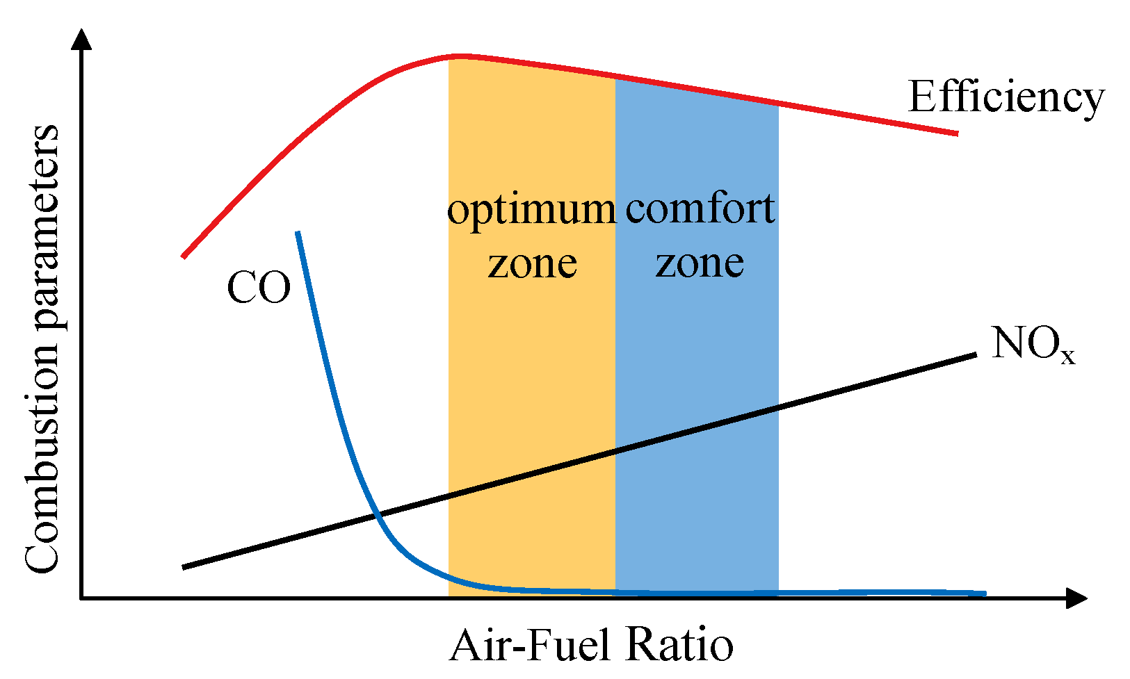
2.1. Conventional Boiler Combustion

Figure 2 shows a typical conventional combustion control with DCL strategy of a coal-fired power plant [5,10,11]. In the figure, each block of F(x) represents a look-up table or static mapping between the input and output. The BMD signal is the output of F₁(x) corresponding to the power load demand, electric power output and main steam pressure. Subsequently, F₂(x) and F₃(x) generate the air flow demand signal and fuel flow demand signal, respectively, based on the predetermined ideal AFR. From the air flow demand signal, the air controller drives the forced draft (FD) fan to control the amount of combustion air into the furnace. Further, with the fuel flow demand signal, the fuel controller drives the primary air fan and pulverizer, accordingly.

The feedback loops with dotted black lines in Figure 2 represent the DCL strategy that prevents the incomplete burning and the excessive combustion air at various loads. Parameters α₁, α₂, α₃ and α₄ are fixed constants of several percent to allow a small margin. This DCL structure is the updated form of the conventional cross-limiting technique that uses α₁ and α₂ loops only, and α₃ and α₄ loops are ignored [5].

The output of F₂(x), the air flow demand, is compared with the output of F₄(x), which is the conversion of fuel flow to air flow. The larger value between the output of F₂(x) and F₄(x) × (1−α₁) was selected to prevent the lack of combustion air in the furnace. In addition, this selector output was compared with F₄(x) × (1 + α₃) and the smaller value was finally selected as the air flow demand to prevent the overfeeding of combustion air in the furnace. In the fuel side, the output of F₃(x) was similarly compared with the output of F₅(x), which is the conversion of air flow to fuel flow. Subsequently, the final fuel flow demand is determined between two margins, α₂ and α₄. The values of α are typically selected between 2% and 5% [5,11]. Therefore, the DCL strategy prevents high or low AFR by selecting appropriate air and fuel flow demands.

2.2. Supplementary DMC for AFR

We implemented the tighter control of the AFR while minimizing its effects on the performance of the existing combustion control system. The DMC supplementary control is applied to the air and fuel flow demands of the conventional multi-loop control, thereby adjusting the amounts of combustion air and fuel to maintain the ideal AFR.

Figure 3 shows the structure of the supplementary control for the AFR using DMC, which is a replacement of the dotted red rectangle in Figure 2. In Figure 3, AFR_k is the air-fuel ratio at the k-th time step, which is the output or controlled variable (CV), and AFR_ref,k is the reference air-fuel ratio at the k-th step; ${\tilde{u}}_{a,k}^{\mathrm{DMC}}$ and ${\tilde{u}}_{f,k}^{\mathrm{DMC}}$ are the plant inputs or manipulated variables (MV) of the proposed DMC, which are the supplementary air flow demand and supplementary fuel flow demand at the k-th step, respectively.

These signals are added to ${\tilde{u}}_{a,k}^{\mathrm{BMD}}$ and ${\tilde{u}}_{f,k}^{\mathrm{BMD}}$, which are, respectively, the air flow and fuel flow demands from the BMD of the conventional multi-loop control. Therefore, the air flow demand ${\tilde{u}}_{a,k}$ and fuel flow demand ${\tilde{u}}_{f,k}$ are the sum of the BMD signals and the supplementary DMC signals as follows:

$${\tilde{u}}_{a,k}={\tilde{u}}_{a,k}^{\mathrm{BMD}}+{\tilde{u}}_{a,k}^{\mathrm{DMC}}$$

(1)

$${\tilde{u}}_{f,k}={\tilde{u}}_{f,k}^{\mathrm{BMD}}+{\tilde{u}}_{f,k}^{\mathrm{DMC}}$$

(2)

The output, AFR_k, is then defined as the ratio:

$${\mathrm{AFR}}_k=u_{a,k}/u_{f,k}$$

(3)

where u_f,k is the fuel flow at the k-th step, which is the output of the pulverizer, and u_a,k is the air flow at the k-th step, which is the sum of the two air flows, from FD fan and primary air fan in Figure 2.

From the viewpoint of practical implementation, this supplementary control structure over the existing multi-loop control logic is very realistic and easy to implement. In an emergency, this type of supplementary control can be easily removed and returned to the conventional multi-loop control system, with which the plant operators are familiar.

Herein, the standard form of the DMC algorithm is used [27]. If we use the standard notation of the plant input and plant output,

$$y_k={\mathrm{AFR}}_k$$

(4)

$${\overline{u}}_k={[{\tilde{u}}_{a,k}^{\mathrm{DMC}},{\tilde{u}}_{f,k}^{\mathrm{DMC}}]}^T$$

(5)

Subsequently, the prediction equation is:

$${\overline{Y}}_{k+1|k}={\overline{Y}}_{k+1|k-1}+\overline{S}\Delta {\overline{U}}_k+{\overline{Y}}_{k+1|k}^d$$

(6)

where

$${\overline{Y}}_{k+1|k}={[{\mathrm{AFR}}_{k+1|k}{\mathrm{AFR}}_{k+2|k}\cdots {\mathrm{AFR}}_{k+p|k}]}^T$$

(7)

$${\overline{Y}}_{k+1|k-1}={[{\mathrm{AFR}}_{k+1|k-1}{\mathrm{AFR}}_{k+2|k-1}\cdots {\mathrm{AFR}}_{k+p|k-1}]}^T$$

(8)

$$\begin{array}{ll}\Delta {\overline{U}}_k& =[\Delta {\overline{u}}_k\Delta {\overline{u}}_{k+1}\cdots \Delta {\overline{u}}_{k+m-1}{]}^T\\ & =[(\Delta {\tilde{u}}_{a,k}^{\mathrm{DMC}},\Delta {\tilde{u}}_{f,k}^{\mathrm{DMC}})\cdots (\Delta {\tilde{u}}_{a,k+m-1}^{\mathrm{DMC}},\Delta {\tilde{u}}_{f,k+m-1}^{\mathrm{DMC}}){]}^T\end{array}$$

(9)

Here, p is the prediction horizon and m is the control horizon; ${\overline{Y}}_{k+1|k}$ is a p × 1 vector, the future output of AFR trajectory at t = k; ${\overline{Y}}_{k+1|k-1}$ is a p × 1 vector, an open-loop prediction of the future output when input u remains at the previous step value u_k−1; ${\overline{Y}}_{k+1|k}^d$ is a p × 1 vector, an estimate of the unmeasured disturbance; $\Delta {\overline{U}}_k$ is a 2 m × 1 input adjustment vector; and $\overline{S}$ is a p × 2 m dynamic matrix including step responses as follows:

$$\overline{S}=\left[\begin{array}{cccc}{\overline{s}}_1& \overline{0}& \cdots & \overline{0}\\ {\overline{s}}_2& {\overline{s}}_1& \ddots & ⋮\\ ⋮& ⋮& \ddots & {\overline{s}}_1\\ ⋮& ⋮& \ddots & ⋮\\ {\overline{s}}_p& {\overline{s}}_{p-1}& \cdots & {\overline{s}}_{p-m+1}\end{array}\right]$$

(10)

$${\overline{s}}_i=\left(s_i^a{s}_i^f\right)$$

(11)

where s_i^a and s_i^f are the step response coefficients of the AFR from the incremented air flow demand and fuel flow demand, respectively, at the i-th sampling step.

To calculate the input adjustment vector, an online quadratic optimization with constraints was performed at every sampling step:

$$\underset{\Delta {\overline{U}}_k}{\min }{\Vert {\overline{E}}_{k+1|k}\Vert }_{\mathsf{\Lambda }}+{\Vert \Delta {\overline{U}}_k\Vert }_{\mathsf{\Gamma }}$$

(12)

where:

$${\overline{E}}_{k+1|k}={\overline{Y}}_{k+1|k}-{\overline{R}}_{k+1|k}={[\begin{array}{cccc}{e}_{k+1|k}& e_{k+2|k}& \cdots & e_{k+p|k}\end{array}]}^T$$

(13)

$${\overline{R}}_{k+1|k}={[\begin{array}{cccc}{\mathrm{AFR}}_{ref,}{}_{k+1|k}& {\mathrm{AFR}}_{ref,}{}_{k+2|k}& \cdots & {\mathrm{AFR}}_{ref,}{}_{k+p|k}\end{array}]}^T$$

(14)

Here, ${\overline{E}}_{k+1|k}$ is a p × 1 error vector, and ${\overline{R}}_{k+1|k}$ is a p × 1 desired trajectory output vector, and Λ and Γ are the weight matrices for the corresponding vectors in the quadratic optimization.

2.3. Constraints of Proposed DMC

An important benefit of using the DMC is the handling of constraints in optimization. Because the DMC herein is supposed to be a supplementary control, additional large changes in the air and fuel demand signal could significantly influence the power output and main steam pressure. Therefore, to minimize its effect on the existing control, the output of the DMC is limited to:

$$-{\mathsf{\beta }}_{\mathrm{a}}\le {\tilde{u}}_{a,k}^{\mathrm{DMC}}\le {\mathsf{\beta }}_{\mathrm{a}}k=1\cdots m$$

(15)

$$-{\mathsf{\beta }}_{\mathrm{f}}\le {\tilde{u}}_{f,k}^{\mathrm{DMC}}\le {\mathsf{\beta }}_{\mathrm{f}}k=1\cdots m$$

(16)

where, β_a and β_f are constants to limit the supplementary air and fuel adjustments, respectively.

It is noteworthy that this supplementary DMC could violate the conventional cross-limit or DCL strategy in Figure 2. Therefore, herein, the DCL strategy is formulated as the constraint in the DMC optimization, i.e., the DCL strategy in the proposed control system is represented as the optimization window at the k-th step as follows:

$$(1-{\mathsf{\alpha }}_1)F_4(u_{f,k})\le {\tilde{u}}_{a,k}^{\mathrm{BMD}}+{\tilde{u}}_{a,k}^{\mathrm{DMC}}\le (1+{\mathsf{\alpha }}_3)F_4(u_{f,k})$$

(17)

$$(1-{\mathsf{\alpha }}_4)F_5(u_{a,k})\le {\tilde{u}}_{f,k}^{\mathrm{BMD}}+{\tilde{u}}_{f,k}^{\mathrm{DMC}}\le (1+{\mathsf{\alpha }}_2)F_5(u_{a,k})$$

(18)

Combining (15)-(18), the two constraints at the k-th step are combined into the following form:

$${\overline{u}}_{\min ,k}\le {\overline{u}}_k\le {\overline{u}}_{\max ,k}$$

(19)

where:

$${\overline{u}}_{\min ,k}=\left(\begin{array}{c}\max \{-{\mathsf{\beta }}_{\mathrm{a}},(1-{\mathsf{\alpha }}_1)F_4(u_{f,k})-{\tilde{u}}_{a,k}^{\mathrm{BMD}}\}\\ \max \{-{\mathsf{\beta }}_{\mathrm{f}},(1-{\mathsf{\alpha }}_4)F_5(u_{a,k})-{\tilde{u}}_{f,k}^{\mathrm{BMD}}\}\end{array}\right)$$

(20)

$${\overline{u}}_{\max ,k}=\left(\begin{array}{c}{\min \text{{}\mathsf{\beta }}_{\mathrm{a}},(1+{\mathsf{\alpha }}_3)F_4(u_{f,k})-{\tilde{u}}_{a,k}^{\mathrm{BMD}}\}\\ {\min \text{{}\mathsf{\beta }}_{\mathrm{f}},(1+{\mathsf{\alpha }}_2)F_5(u_{a,k})-{\tilde{u}}_{f,k}^{\mathrm{BMD}}\}\end{array}\right)$$

(21)

Therefore, the constraints for the 2 m × 1 input vector is

$$\left[\begin{array}{c}{\overline{u}}_{\min ,k}\\ \left(\begin{array}{c}-{\mathsf{\beta }}_{\mathrm{a}}\\ -{\mathsf{\beta }}_{\mathrm{f}}\end{array}\right)\\ ⋮\\ \left(\begin{array}{c}-{\mathsf{\beta }}_{\mathrm{a}}\\ -{\mathsf{\beta }}_{\mathrm{f}}\end{array}\right)\end{array}\right]\le {\overline{U}}_k\le \left[\begin{array}{c}{\overline{u}}_{\max ,k}\\ \left(\begin{array}{c}{\mathsf{\beta }}_{\mathrm{a}}\\ {\mathsf{\beta }}_{\mathrm{f}}\end{array}\right)\\ ⋮\\ \left(\begin{array}{c}{\mathsf{\beta }}_{\mathrm{a}}\\ {\mathsf{\beta }}_{\mathrm{f}}\end{array}\right)\end{array}\right]$$

(22)

For the quadratic programming problem of (12), the constraints need to be changed into the standard linear inequality form:

$${\overline{C}}_k\Delta {\overline{U}}_k\ge {\overline{D}}_k$$

(23)

where ${\overline{C}}_k$ and ${\overline{D}}_k$ are constant matrixes. Therefore, (22) should be represented in the form of (23). From the definition of difference,

$${\overline{u}}_k={\overline{u}}_{k-1}+\Delta {\overline{u}}_k$$

(24)

$${\overline{u}}_{k+l}={\overline{u}}_{k-1}+{\displaystyle \sum _{i=0}^l{\overline{u}}_{k+i}},\hspace{1em}l=0,1,\cdots ,m-1$$

(25)

(22) is represented as:

$$\left[\begin{array}{c}{\overline{u}}_{\min ,k}-{\overline{u}}_{k-1}\\ -\left(\begin{array}{c}{\mathsf{\beta }}_{\mathrm{a}}\\ {\mathsf{\beta }}_{\mathrm{f}}\end{array}\right)-{\overline{u}}_{k-1}\\ ⋮\\ -\left(\begin{array}{c}{\mathsf{\beta }}_{\mathrm{a}}\\ {\mathsf{\beta }}_{\mathrm{f}}\end{array}\right)-{\overline{u}}_{k-1}\end{array}\right]\le \left[\begin{array}{c}\Delta {\overline{u}}_k\\ {\displaystyle \sum _{i=0}^l\Delta {\overline{u}}_{k+i}}\\ ⋮\\ {\displaystyle \sum _{i=0}^l\Delta {\overline{u}}_{k+i}}\end{array}\right]\le \left[\begin{array}{c}{\overline{u}}_{\max ,k}-{\overline{u}}_{k-1}\\ \left(\begin{array}{c}{\mathsf{\beta }}_{\mathrm{a}}\\ {\mathsf{\beta }}_{\mathrm{f}}\end{array}\right)-{\overline{u}}_{k-1}\\ ⋮\\ \left(\begin{array}{c}{\mathsf{\beta }}_{\mathrm{a}}\\ {\mathsf{\beta }}_{\mathrm{f}}\end{array}\right)-{\overline{u}}_{k-1}\end{array}\right]$$

(26)

The middle term of (26) is represented as:

$$\left[\begin{array}{c}\Delta {\overline{u}}_k\\ {\displaystyle \sum _{i=0}^1\Delta {\overline{u}}_{k+i}}\\ ⋮\\ {\displaystyle \sum _{i=0}^l\Delta {\overline{u}}_{k+i}}\end{array}\right]=\left[\begin{array}{cccc}\overline{I}& \overline{0}& \cdots & \overline{0}\\ \overline{I}& \overline{I}& \overline{0}& ⋮\\ ⋮& ⋮& \ddots & \overline{0}\\ \overline{I}& \overline{I}& \overline{I}& \overline{I}\end{array}\right]\left[\begin{array}{c}\Delta {\overline{u}}_k\\ \Delta {\overline{u}}_{k+1}\\ ⋮\\ \Delta {\overline{u}}_{k+m-1}\end{array}\right]={\overline{I}}_L\left[\begin{array}{c}\Delta {\overline{u}}_k\\ \Delta {\overline{u}}_{k+1}\\ ⋮\\ \Delta {\overline{u}}_{k+m-1}\end{array}\right]$$

(27)

where $\overline{I}$ is a 2 × 2 identity matrix, and ${\overline{I}}_L$ is a 2 m × 2 m matrix. Finally, (26) is represented as follows:

$$\left[\begin{array}{c}{\overline{I}}_L\\ -{\overline{I}}_L\end{array}\right]\Delta {\overline{U}}_k\ge \left[\begin{array}{c}\begin{array}{c}{\overline{u}}_{\min ,k}-\left(\begin{array}{c}{\tilde{u}}_{a,k-1}^{\mathrm{DMC}}\\ {\tilde{u}}_{f,k-1}^{\mathrm{DMC}}\end{array}\right)\\ \left(\begin{array}{c}-{\mathsf{\beta }}_{\mathrm{a}}-{\tilde{u}}_{a,k-1}^{\mathrm{DMC}}\\ -{\mathsf{\beta }}_{\mathrm{f}}-{\tilde{u}}_{f,k-1}^{\mathrm{DMC}}\end{array}\right)\\ ⋮\\ \left(\begin{array}{c}-{\mathsf{\beta }}_{\mathrm{a}}-{\tilde{u}}_{a,k-1}^{\mathrm{DMC}}\\ -{\mathsf{\beta }}_{\mathrm{f}}-{\tilde{u}}_{f,k-1}^{\mathrm{DMC}}\end{array}\right)\end{array}\\ \begin{array}{c}\left(\begin{array}{c}{\tilde{u}}_{a,k-1}^{\mathrm{DMC}}\\ {\tilde{u}}_{f,k-1}^{\mathrm{DMC}}\end{array}\right)-{\overline{u}}_{\max ,k}\\ \left(\begin{array}{c}{\tilde{u}}_{a,k-1}^{\mathrm{DMC}}-{\mathsf{\beta }}_{\mathrm{a}}\\ {\tilde{u}}_{f,k-1}^{\mathrm{DMC}}-{\mathsf{\beta }}_{\mathrm{f}}\end{array}\right)\\ ⋮\\ \left(\begin{array}{c}{\tilde{u}}_{a,k-1}^{\mathrm{DMC}}-{\mathsf{\beta }}_{\mathrm{a}}\\ {\tilde{u}}_{f,k-1}^{\mathrm{DMC}}-{\mathsf{\beta }}_{\mathrm{f}}\end{array}\right)\end{array}\end{array}\right]$$

(28)

Therefore, both the DCL strategy and the supplementary control limits are represented in the standard form of (23) in the proposed DMC. The constraint of (28) in the proposed supplementary DMC is used in the standard online optimization of (12) at every sampling step.

3. Applications to Power Plants

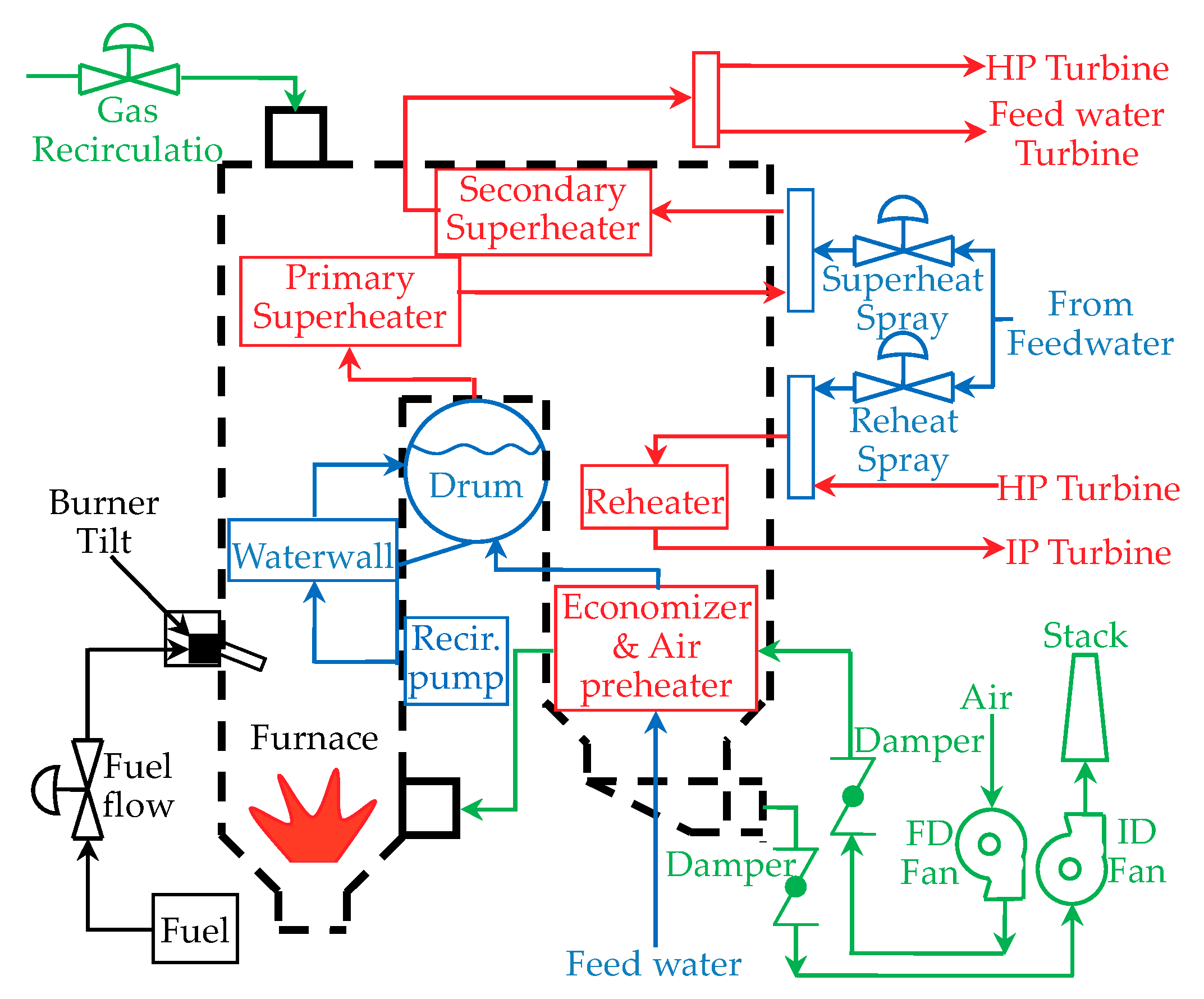
3.1. 600-MW Drum-Type Thermal Power Plant

Figure 4 shows the boiler system of a 600-MW oil-fired drum-type thermal power plant model. Each component of the model is developed with mass, momentum, and energy balance equations. This nonlinear power plant model was applied and validated in many studies [25,28,29].

The combustion control system of this plant primarily follows the standard structure of the coal-fired plant in Figure 2. Because this model is an oil-fired plant, the fuel flow demand signal manipulates the fuel flow valve in Figure 4 instead of the pulverizer and primary air fan in Figure 2. Therefore, u_f,k is the output of the fuel flow valve in this plant. The conventional cross-limiting algorithm is equipped in this model, and both α₁ and α₂ were set to 5%.

Figure 5 shows the response of the AFR as a result of the step increments of ${\tilde{u}}_a^{\mathrm{DMC}}$ and ${\tilde{u}}_f^{\mathrm{DMC}}$ at t = 0 from the steady state of 450 MW. The 1% of the normal operation range is used independently for the two step inputs. Because this is a closed-loop test for supplementary control, these transient responses include the dynamics of not only the power plant model but also the existing multi-loop control logics. In Figure 5, from the initial value 15.35, the AFR is finally increased/decreased to 15.57/15.12 due to the increase in combustion air/fuel, respectively.

The tuning of the DMC parameters is important. Theoretically, a small sampling time and a large prediction and control horizons are desirable from the view point of control performance. However, this increases the computational burden in practice. The sampling time is determined as 1 s. Therefore, the responses of Figure 5 were sampled at every 1 s and stored in the step-response matrix $\overline{S}$. The error and input increments in (12) are:

$$\Vert e_{k+1|k}\Vert ={[e_{k+1|k}]}^T[\mathsf{\Lambda }][e_{k+1|k}]$$

(29)

$$\Vert \Delta {\overline{u}}_k\Vert ={\left[\begin{array}{c}\Delta {\tilde{u}}_{a,k}^{\mathrm{DMC}}\\ \Delta {\tilde{u}}_{f,k}^{\mathrm{DMC}}\end{array}\right]}^T\left[\begin{array}{cc}{\mathsf{\Gamma }}_a& 0\\ 0& {\mathsf{\Gamma }}_f\end{array}\right]\left[\begin{array}{c}\Delta {\tilde{u}}_{a,k}^{\mathrm{DMC}}\\ \Delta {\tilde{u}}_{f,k}^{\mathrm{DMC}}\end{array}\right]$$

(30)

where Λ is the weight of the AFR error; Γ_a is the weight of $\Delta {\tilde{u}}_{a,k}^{\mathrm{DMC}}$ ; and Γ_f is the weight of $\Delta {\tilde{u}}_{f,k}^{\mathrm{DMC}}$. The DMC parameters are listed in

Table 1. DMC parameters of 600 MW drum-type thermal power plant.

Λ	Γa	Γf	p	m	βa	βf
1	1	10	300	100	2%	1.25%

. The p is selected as 300 [s] for AFR response to settle down in Figure 5. The m is selected as 100 [s] considering computational burden. A small β limits the performance of proposed supplementary control, while a large β can affect the other control loops. By trial and error, to limit excessive control action, β_a and β_f were selected as 2% and 1.25% of their normal operation ranges, respectively. Because of the small β_f, this supplementary DMC primarily manipulates the combustion air flow demand rather than the fuel demand.

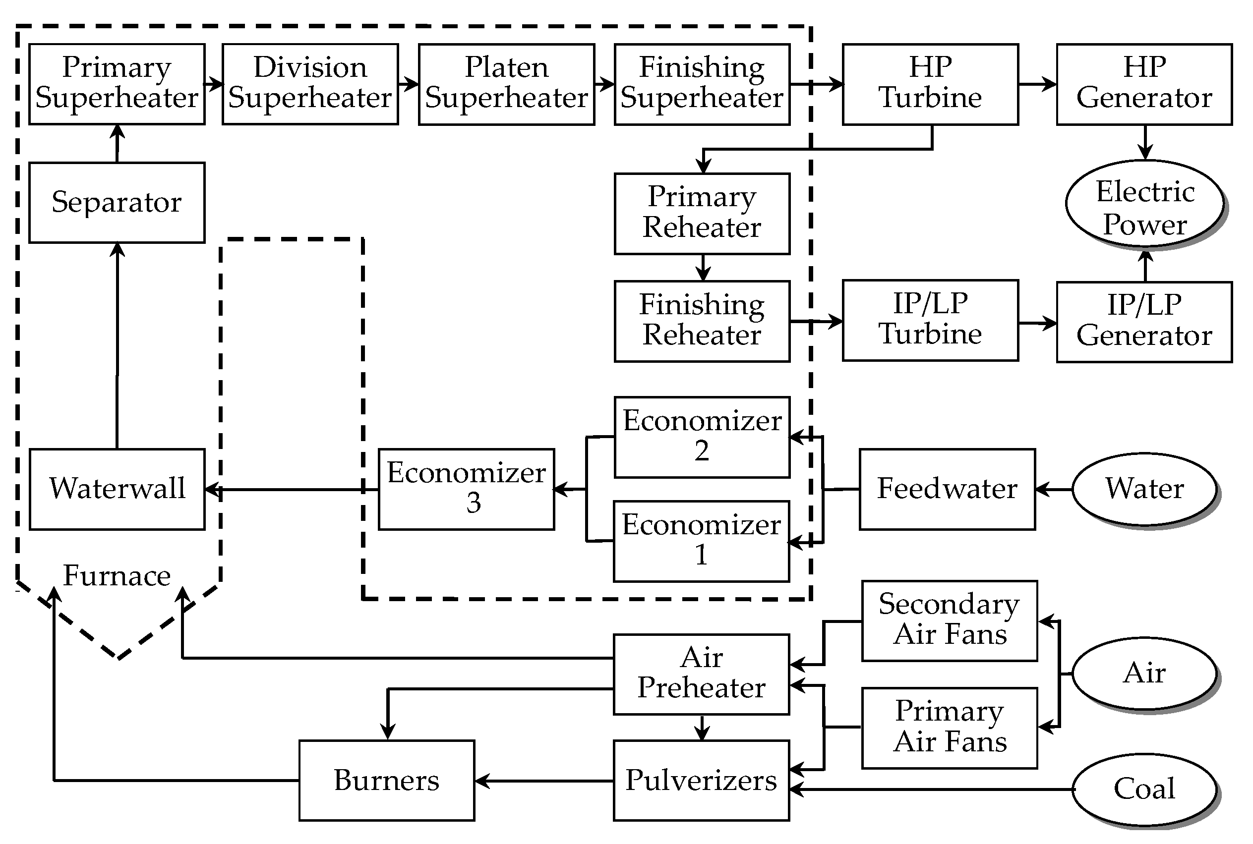
3.2. 1000-MW Once-Through Type Thermal Power Plant

Figure 6 is the dynamic boiler simulation model (DBSM) of the 1000 MW ultra-supercritical (USC) coal-fired once-through type model. This nonlinear model was also developed based on mass, momentum, and energy balances. It is a field-proven simulator for the power plant control logic design in industry [26,30,31].

In Figure 6, the secondary air fan represents the FD fan in Figure 2 to control the amount of combustion air. The combustion control system of this plant primarily follows the standard structure in Figure 2. The conventional cross-limiting algorithm is equipped in this model, and the values of α₁ and α₂ were set to 5%.

Figure 7 shows the step response of the AFR as a result of the step increase of ${\tilde{u}}_a^{\mathrm{DMC}}$. One percent of the normal operation range of ${\tilde{u}}_a^{\mathrm{DMC}}$ was applied at the steady state of 825 MW. The AFR increased from 11.12 to 11.26 due to the increase in combustion air. A faster transient response was observed compared to the response in Figure 5. This faster response can be interpreted as the faster dynamics of the once-through-type boiler compared to that of the drum-type boiler.

Figure 8 shows the step response of the AFR for a 1% step increase of ${\tilde{u}}_f^{\mathrm{DMC}}$ in the steady state of 825 MW. The AFR is decreased from 11.12 to 10.97 in steady state. The slower response than that of Figure 7 can be attributed to the slow dynamics of the pulverizer. Therefore, in this study, ${\tilde{u}}_a^{\mathrm{DMC}}$ is primarily used for MV to achieve a fast control response.

The same structure of the DMC was applied to this plant. The sampling time was selected as 1 s and the DMC weight parameters are shown in

Table 2. DMC parameters of 1000 MW once through-type thermal power plant.

Λ	Γa	Γf	p	m	βa	βf
10	1	0.1	300	100	1.36%	0.02%

. The p was selected as 300 s for AFR to settle down in Figure 8. The m was also selected as 100 s considering computational burden. For this plant, β_a and β_f were selected as 1.36% and 0.02% by trial and error, respectively. Because of the small β_f, this supplementary DMC primarily manipulates the combustion air flow demand rather than the fuel demand.

4. Simulation Results

4.1. Simulation of 600-MW Drum-Type Thermal Power Plant

The DMC supplementary control is developed in the MATLAB environment. In this simulation, the control performance (12) with constraints (28) is optimized by the quadratic programming, MATLAB function “quadprog ( )”, at every sampling time.

The simulation scenario has two step changes for the electric power load demand in Figure 9. The load demand change is limited to 0.5 MW/s, which is 5% per minute of the total load. In this simulation, for simplicity, the ideal AFR of the drum-type plant model is assumed to be constant, i.e., 15.35 at every electric power load.

To confirm the effect of the proposed supplementary control on the main control loop, two responses of the electric power output are compared in Figure 9, with and without DMC. Because the supplementary control signal is limited by β_a and β_f, which are only 2% and 1.25% of their normal operation ranges, respectively, two responses are almost the same, and the proposed supplementary control does not affect the existing multi-loop control system operation.

Figure 10 shows the comparison of the AFR between the conventional multi-loop control and the proposed DMC supplementary control during the transient. Although the responses of the electric power output are similar, the AFR of the proposed DMC shows a tighter control during the transient of the load changes.

Table 3. Squared error sum comparison of AFR in 600 MW plant.

Multi-Loop	23.069
DMC	1.137
Percentage of DMC/Multi-loop	4.93%

shows that the squared error sum of the conventional control can be significantly reduced, to 4.93%, by the proposed supplementary control. Therefore, the environmental emissions by the conventional control during the transient of the load change can be effectively reduced by the proposed supplementary DMC.

Figure 11 and Figure 12 show the movements of the DMC control signals ${\tilde{u}}_{a,k}^{\mathrm{DMC}}$ and ${\tilde{u}}_{f,k}^{\mathrm{DMC}}$, respectively. In the figures, supplementary control limits of ±2% and ±1.25% are represented as ±12.50 kg/s and ±0.51 kg/s, respectively. During the first 50 [s] in Figure 10, a large AFR was expected by the DMC prediction of (6). Then, optimization of (12) with constraint of (28) was calculated to keep the AFR to be 15.35, based on the step-response model of (10) which is developed from Figure 5. As a result of optimization of (12), the supplementary signals ${\tilde{u}}_{a,k}^{\mathrm{DMC}}$ and ${\tilde{u}}_{f,k}^{\mathrm{DMC}}$ were calculated. The ${\tilde{u}}_{a,k}^{\mathrm{DMC}}$ is negative in Figure 11, while ${\tilde{u}}_{f,k}^{\mathrm{DMC}}$ is positive in Figure 12 to reduce the AFR. This control process is repeated at every sampling step in DMC. Accordingly, the AFR of the proposed control is reduced in the first 50 s as shown in Figure 10, and excessive NOx and stack heat loss can be reduced with the proposed supplementary control.

To confirm the DCL logic of the proposed DMC, the air side optimization window (17) in the first 200 s is represented in Figure 13. In the figure, the lower bound “DCL min” is (1−α₁) F₄(u_f,k), the upper bound “DCL max” is (1 + α₃) F₄(u_f,k), and ${\tilde{u}}_{a,k}$ is ${\tilde{u}}_{a,k}^{\mathrm{BMD}}+{\tilde{u}}_{a,k}^{\mathrm{DMC}}$. At approximately 10 s and 110 s, the amplitude of ${\tilde{u}}_{a,k}^{\mathrm{DMC}}$ was effectively restricted for ${\tilde{u}}_{a,k}$ to stay within the optimization window constrained by the DCL logic in (28).

4.2. Simulation of 1000-MW Once-Through Type Thermal Power Plant

The DMC supplementary control was also developed for the 1000-MW once-through type unit in MATLAB and linked with the DBSM simulator. The simulation scenario contains two step changes of the power load demand, where the load demand is reduced from 825 MW to 750 MW at 0 s, and increased to 950 MW at 1500 s. The load demand change at each sampling time is also restricted by the internal logic of the DBSM. Unlike the 600-MW drum-type plant, the ideal AFR of the DBSM is not a constant but is specified by the internal logic of the DBSM as a function of the load. In this simulation, the ideal AFR of the DBSM is used as the AFR_ref,k for the DMC.

Though they are not represented in this paper, the power output and main steam pressure of the two controls are almost the same, therefore, the proposed supplementary control does not affect the existing multi-loop control system operation. Figure 14 shows the ideal AFR of the DBSM, the AFR of the conventional multi-loop control, and the AFR of the proposed DMC. Figure 15 shows the variation of ${\tilde{u}}_{a,k}^{\mathrm{DMC}}$. In the figure, the supplementary control of ${\tilde{u}}_{a,k}^{\mathrm{DMC}}$ is limited with ±14.30 kg/s, which is ±1.36% of the normal operation range. The variation of ${\tilde{u}}_{f,k}^{\mathrm{DMC}}$ is not represented because it is limited with a small β_f. Although it is not shown, the DMC controls satisfies the optimization window constrained by the DCL logic in (28).

In Figure 14, the responses of the second step change between 1500 s and 1750 s show the clear comparison between the two controls. A large AFR of the conventional control can be reduced by the proposed DMC. Accordingly, NOx emissions can be reduced at the same time. The numerical comparison is shown in

Table 4. Squared error sum comparison of AFR in 1000 MW plant.

Multi-loop	8.613
DMC	1.237
Percentage of DMC/ Multi-loop	14.36%

. For the once-through type plant, the squared error sum was reduced to 14.36% with the proposed supplementary DMC.

5. Conclusions

In this paper, we proposed a supplementary DMC for tighter control of the AFR to reduce the environmental emissions of thermal power plants. Two manipulated variables of the DMC are the air flow demand and fuel flow demand. The amplitudes of the supplementary control signals are limited by the DMC constraints to minimize the effect on the main control loops of power plants, while optimized within the optimization window constrained by the conventional DCL logic.

Simulations considered two different types of power plants, which are 600-MW drum-type oil fired plant and 1000 MW once-through type coal-fired plant. Without affecting existing power plant operation, the proposed supplementary DMC shows very tight control of the AFR in transient period. Therefore, the reduction in environmental emissions in various thermal power plants can be expected.

Because the supplementary structure maintains the existing multi-loop control, the proposed control can be directly applied to the currently operating power plant. In addition, since the plant operator can easily return to the original multi-loop control logic, it can cope easily with emergency situations.

For practical implementation, the number of adjustable parameters of DMC is quite high and an additional computer server might be necessary over the exiting DCS (distributed control system). Therefore, future research could investigate a simpler control structure as a supplementary control which can be implemented into DCS of practical power plant.

References

1. Lewtas, J. Air pollution combustion emissions: Characterization of causative agents and mechanisms associated with cancer, reproductive, and cardiovascular effects. Rev. Mutat. Res. 2007, 636, 95–133. [Google Scholar] [CrossRef] [PubMed]
2. Streets, D.G.; Waldhoff, S.T. Present and future emissions of air pollutants in China: SO2, NOx and CO. Atmos. Environ. 2000, 34, 363–374. [Google Scholar] [CrossRef]
3. Wiatros-Motyka, M. Optimising Fuel Flow in Pulverised Coal and Biomass-Fired Boilers; IEA Clean Coal Centre: London, UK, 2016. [Google Scholar]
4. Li, S.; Xu, T.; Hui, S.; Wei, X. NOx emission and thermal efficiency of a 300MWe utility boiler retrofitted by air staging. Appl. Energy 2009, 86, 1797–1803. [Google Scholar] [CrossRef]
5. Dukelow, S.G. The Control of Boilers; Instrument Society of America, Research Triangle Park: North Carolina, USA, 1986. [Google Scholar]
6. Wang, Y.; Yu, X. New coordinated control design for thermal-power-generation units. IEEE Trans. Ind. Electron. 2010, 57, 3848–3856. [Google Scholar] [CrossRef]
7. Wei, L.; Fang, F. H∞-LQR-based coordinated control for large coal-fired boiler–turbine generation units. IEEE Trans. Ind. Electron. 2017, 64, 5212–5221. [Google Scholar] [CrossRef]
8. Takiyama, T.; Shiomi, E.; Morita, S. Air–fuel ratio control system using pulse width and amplitude modulation at transient state. JSAE Rev. 2001, 22, 537–544. [Google Scholar] [CrossRef]
9. Bhowmick, M.; Bera, S.C. An approach to optimum combustion control using parallel type and cross-limiting type technique. J. Process Control 2012, 22, 330–337. [Google Scholar] [CrossRef]
10. Liu, Z.H.; He, G.X.; Wang, L.Z. Optimization of furnace combustion control system based on double cross-limiting strategy. In Proceedings of the 2010 International Conference on Intelligent Computation Technology and Automation, Changsha, China, 11–12 May 2010; pp. 858–861. [Google Scholar]
11. Zanoli, S.M.; Barchiesi, D.; Astolfi, G.; Barboni, L. Advanced control solutions to increase efficiency of a furnace combustion process. In Proceedings of the European Control Conference (ECC), Zurich, Switzerland, 17–19 July 2013; pp. 4316–4321. [Google Scholar]
12. Hou, Z.; Xiong, S. On Model-Free Adaptive Control and its Stability Analysis. IEEE Trans. Auto. Control 2019. [Google Scholar] [CrossRef]
13. Bara, O.; Fliess, M.; Join, C.; Day, J.; Djouadi, S.M. Toward a model–free feedback control synthesis for treating acute inflammation. J. Theor. Biol. 2018, 478, 26–37. [Google Scholar] [CrossRef] [Green Version]
14. Safaei, A.; Mahyuddin, M.N. Optimal model–free control for a generic MIMO nonlinear system with application to autonomous mobile robots. Int. J. Adapt. Control Signal Process. 2018, 32, 792–815. [Google Scholar] [CrossRef]
15. Lee, S.D.; Bae, Y.G.; Jung, S. A Decentralized Model Identification Scheme by Random-walk RLS Process for Robot Manipulators: Experimental Studies. J. Control Autom. Syst. 2019, 17, 1856–1865. [Google Scholar] [CrossRef]
16. Roman, R.C.; Precup, R.E.; Radac, M.B. Model–free fuzzy control of twin rotor aerodynamic systems. In 2017 25th Mediterranean Conference on Control and Automation (MED); IEEE: Valletta, Malta, 2017; pp. 559–564. [Google Scholar]
17. Precup, R.E.; Radac, M.B.; Roman, R.C.; Petriu, E.M. Model–free sliding mode control of nonlinear systems: Algorithms and experiments. Inf. Sci. 2017, 381, 176–192. [Google Scholar] [CrossRef]
18. Roman, R.C.; Precup, R.E.; David, R.C. Second Order Intelligent Proportional-Integral Fuzzy Control of Twin Rotor Aerodynamic System. Procedia Comput. Sci. 2019, 139, 372–380. [Google Scholar] [CrossRef]
19. Kim, D.; Oh, H.S.; Moon, I.C. Black-box Modeling for Aircraft Maneuver Control with Bayesian Optimization. J. Control Autom. Syst. 2019, 17, 1558–1568. [Google Scholar] [CrossRef]
20. Roman, R.C.; Radac, M.B.; Precup, R.E.; Petru, E.M. Virtual reference feedback tuning of model–free control algorithms for servo systems. Machines 2017, 5, 25. [Google Scholar] [CrossRef]
21. Qin, S.; Badgwell, T. A survey of industrial model predictive control technology. Control Eng. Pract. 2003, 11, 733–764. [Google Scholar] [CrossRef]
22. Gracia, C.E.; Prett, D.M.; Morari, M. Model predictive control: Theory and practice−A survey. Automatica 1989, 25, 335–348. [Google Scholar] [CrossRef]
23. Lee, J.H. Model predictive control in the process industries: Review, current status and future outlook. In Proceedings of the 2nd Asian Control Conference, Seoul, Korea, 22–25 July 1997; pp. 435–438. [Google Scholar]
24. Moon, U.C.; Lee, K.Y. Step-response model development for dynamic matrix control of a drum-type boiler-turbine system. IEEE Trans. Energy Convers. 2009, 24, 423–430. [Google Scholar] [CrossRef]
25. Moon, U.C.; Lee, Y.; Lee, K.Y. Practical dynamic matrix control for thermal power plant coordinated control. Control Eng. Pract. 2018, 71, 154–163. [Google Scholar] [CrossRef]
26. Lee, Y.; Yoo, E.; Lee, T.; Moon, U.C. Supplementary control of conventional coordinated control for 1000MW ultra-supercritical thermal power plant using dynamic matrix control. J. Electr. Eng. Technol. 2018, 13, 97–104. [Google Scholar]
27. Moon, U.C.; Lee, K.Y. An adaptive dynamic matrix control with fuzzy-interpolated step-response model for a drum-type boiler-turbine system. IEEE Trans. Energy Convers. 2011, 26, 393–401. [Google Scholar] [CrossRef]
28. Usoro, P.B. Modeling and Simulation of a Drum Boiler-Turbine Power Plant under Emergency State Control. Master’s Thesis, Massachusetts Institute. Technology, Cambridge, MA, USA, May 1977. [Google Scholar]
29. Heo, J.S.; Lee, K.Y. A multiagent-system-based intelligent reference governor for multiobjective optimal power plant operation. IEEE Trans. Energy Convers. 2008, 23, 1082–1092. [Google Scholar] [CrossRef]
30. Lee, K.Y.; Van Sickel, J.H.; Hoffman, J.A.; Jung, W.H.; Kim, S.H. Controller design for a large-scale ultrasupercritical once-through boiler power plant. IEEE Trans. Energy Convers. 2010, 25, 1063–1070. [Google Scholar] [CrossRef]
31. Go, G.; Moon, U.C. A water-wall model of supercritical once-through boilers using lumped parameter method. J. Electr. Eng. Technol. 2014, 9, 1900–1908. [Google Scholar] [CrossRef] [Green Version]
Figure 1. Emissions and efficiency as a function of air–fuel ratio.
Energies 13 00226 g001
Figure 2. Typical power plant combustion with double cross-limiting strategy.
Energies 13 00226 g002
Figure 3. Proposed control system configuration.
Energies 13 00226 g003
Figure 4. Boiler system of a 600-MW drum-type thermal power plant.
Energies 13 00226 g004
Figure 5. Step responses in a 600 MW power plant.
Energies 13 00226 g005
Figure 6. Schematic of a 1000 MW once-through-type thermal power plant.
Energies 13 00226 g006
Figure 7. Response of air–fuel ratio in 1000 MW plant due to step increase of u ˜ a DMC .
Energies 13 00226 g007
Figure 8. Response of air–fuel ratio in 1000 MW plant due to step increase of u ˜ f DMC .
Energies 13 00226 g008
Figure 9. Comparison of electric power output of 600-MW plant.
Energies 13 00226 g009
Figure 10. Comparison of AFR in 600-MW plant.
Energies 13 00226 g010
Figure 11. DMC supplementary air flow demand of 600-MW plant.
Energies 13 00226 g011
Figure 12. DMC supplementary fuel flow demand of 600-MW plant.
Energies 13 00226 g012
Figure 13. Optimization window for air flow demand signal of DMC for 600-MW plant.
Energies 13 00226 g013
Figure 14. Comparison of air in 1000-MW plant.
Energies 13 00226 g014
Figure 15. DMC supplementary air flow demand of 1000 MW plant.
Energies 13 00226 g015