Abstract
Accurate temperature estimation inside an electrical motor is key for condition monitoring, fault detection, and enhanced end-of-life duration. Additionally, thermal information can benefit motor control to improve operational performance. Lumped-parameter thermal networks (LPTNs) for electrical machines are both flexible and cost-effective in computation time, which makes them attractive for use in real-time condition monitoring and integration in motor control. However, the accuracy of these thermal networks heavily depends on the accuracy of its system parameters, some of which are difficult to calculate analytically or even empirically and need to be determined experimentally. In this paper, a methodology for the thermal condition monitoring of long-duration transient and steady-state temperatures in an induction motor is presented. To achieve this goal, a computationally efficient second-order LPTN for a 5.5 kW squirrel-cage induction motor is proposed to apprehend the dominant heat paths. A fully thermally instrumented induction motor has been prepared to collect spatial and temporal temperature information. Using the experimental stator and rotor temperature data collected at different motor operating speeds and torques, the key thermal parameter values in the LPTN are identified by means of an inverse methodology that aligns the simulated temperatures of the stator windings and rotor with the corresponding measured temperatures. Validation results show that the absolute average thermal modelling error does not exceed 1.45 °C with maximum absolute error of 2.10 °C when the motor operates at fixed speed and torque. During intermittent motor-loading operation, a mean (maximum) stator temperature error of 0.38 °C (0.92 °C) was achieved and mean (maximum) rotor errors of 2.11 °C (3.40 °C). These results show the validity of the proposed thermal model but also its ability to predict in real time the temperature variations in stator and rotor for condition monitoring and motor control.
1. Introduction
Thermal prediction of electric motors is becoming increasingly important in the drive for higher power density, energy efficiency and cost reduction [1]. Accurate temperature estimation of motor hotspots is key for condition monitoring and fault detection [2], as well as motor control [3,4]. As the stator windings are surrounded by thermally vulnerable insulation material, real-time prediction of the temperature of the windings allows enhancement of the motor end-of-life duration. Furthermore, Direct Torque Control (DTC) schemes for electric motors depend on the parameter value of the stator resistance, especially at low speeds or standstill [3]. A large portion of the industrial induction motors use Field-Oriented Control (FOC) schemes. They rely on having accurate knowledge of the rotor resistance parameter value for their torque control [4]. Having accurate real-time temperature prediction capabilities thus allows improvement to the torque performance of DTC (i.e., knowledge of the stator windings temperature) and FOC (rotor temperature) as well as enhance end-of-life duration.
Thermal analysis of electric machines is a less elaborated field of research, although considerable advancements have been achieved over the past three decades. Three large categories can be distinguished to model the thermal behavior of electric motors: a fully numerical approach, a lumped-parameter thermal network (LPTN) approach, or a combination of both. Fully numerical methods include rigorous analyses using Finite-Element (FE) methods both for determining heat transfer through solid materials and for electromagnetic loss determination, while computational fluid dynamics are used to model convective heat transfer between the motor and coolant fluid or air [5,6,7]. The main advantage of these methods is the capability to accurately estimate the entire temperature distribution of the motor, including critical hot-spot locations [1]. These models are however unsuitable for real-time applications due to their high computational cost.
Contrary to FE-based models, LPTNs are computationally cost efficient, which makes them suitable for real-time applications. They have been introduced in [8] and developed [9,10,11,12] over recent years. A combination of LPTN and FE has been proposed and used in [13,14]. The challenge with LPTN modelling is the identification of on the one hand the dominant heat paths [1] and on the other hand the thermal parameter values of the LPTN elements, which have a considerable impact on the accuracy of temperature prediction [15,16]. These thermal parameters can either be calculated in a direct manner through analytical relations and empirical formulas from literature [16,17,18,19], or alternatively be determined through an inverse methodology by using temperature measurements as a reference for the model outputs [11,20,21,22,23,24,25].
The bulk of research work concerning electric motor LPTNs use the direct method to identify the thermal system parameters. Simplifications to the original network in [8] have been presented in [17] for a self-ventilated induction motor, taking into consideration only the steady-state regime where maximal temperature deviations of 5 °C were achieved. A similar thermal analysis was performed in [9] for high power density electrical machines for steady-state regime, where the electromagnetic losses were calculated using FE methods, while air gap convection was calculated analytically using empirical expressions based on the relevant dimensionless numbers. Transient thermal behavior of an induction motor using a second-order LPTN is investigated for only one motor operating point in [26], where mechanical losses were also included in the model, leading to temperature modelling errors of only 0.75 °C. Furthermore, in [27] the authors adapted the network introduced in [8] to a maximum-based temperature instead of an average-based temperature model, using FE calculations as a reference. Another addition to the original model has been considered in [19], where nodes are supplemented in the LPTN to apprehend the heat transport by air flow in an open-type, air-cooled induction motor. In this case, computational fluid dynamics calculations validated the full thermal model. However, only steady-state regime was considered since thermal capacitances were absent. A higher-order LPTN was considered for the thermal analysis of an induction motor with a die cast copper rotor in [18], where it was shown that the stator end winding transient temperature could be predicted for different motor loadings, although the maximal modelling error was still close to 5 °C. Finally, in [12,28] the short-time transient behavior of the stator windings of an induction motor was examined for the first few minutes of operation.
In this work, a methodology for the thermal condition monitoring of long-duration transient and steady-state temperatures in an induction motor is presented. To achieve this goal, a computationally efficient second-order LPTN for a 5.5 kW squirrel-cage induction motor is proposed to apprehend the dominant heat paths. A fully thermally instrumented induction motor has been prepared to collect spatial and temporal temperature information. This induction motor is connected in a back-to-back configuration with another induction motor that emulates the load. Using the experimental stator and rotor temperature data collected at different motor operating speeds and torques, the key thermal parameter values in the LPTN are identified by means of an inverse methodology. The capability to predict both long-duration transient and steady-state temperatures of stator windings and rotor cage is tested and validated experimentally for both fixed and intermittent motor operations. The proposed methods have the potential to be included in a condition monitoring system for induction motors that are not fully instrumented.
Section 2 details the structure and analytical discussion of the proposed LPTN. Section 3 discusses the experimental setup with the fully thermally instrumented induction motor. The next Section 4 presents the inverse methodology for the thermal identification of the induction motor. Section 5 discusses the experimental identification of the proposed LPTN and its subsequent validation for both different fixed motor operating points and intermittent operating regime. Finally, conclusions are drawn in Section 6.
2. Lumped-Parameter Thermal Network
A second-order LPTN is considered to model the temperature of the stator windings and the rotor block in an induction motor. It is assumed in this thermal model that both the copper stator windings and the rotor cylinder block are at a uniform temperature [29,30]. The model is illustrated in Figure 1, where the nodes and represent the temperature of the stator windings and rotor, respectively. The thermal capacity of the stator windings and rotor are denoted with and , respectively, while the heat sources due to motor losses are specified as and , respectively. is the thermal resistance between stator windings and the ambient air at room temperature and is the thermal resistance between the rotor and the copper stator windings.
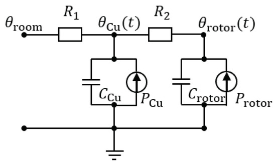
Figure 1.
Illustration of the second-order LPTN to model the temperature of the copper stator windings and the rotor cylinder.
The thermal behavior can be described by the following differential equation:
where is the vector carrying the temperature of the stator windings and rotor, is the time derivative of , is the thermal capacity matrix, is the thermal admittance matrix and the vector carrying the thermal heat sources. Equation (1) can be written in its full form as follows:
where T and are the motor torque and speed, respectively. The motor speed has a considerable influence on the thermal resistance , as it includes the modelling of heat transfer through convection between the rotor, the air gap and the stator. The heat sources and represent the motor joule and iron losses, and are dependent on the motor operating points of torque and speed. These quantities can be explicitly written as function of motor torque T and speed :
where the p coefficients are fitting parameters that need to be determined experimentally. Equation (1) can be written in the standard form for state-space equations as follows:
The full solutions for and can be obtained by superposition of the zero-input response and zero-state response :
The zero-input response and zero-state response are:
where the and coefficients are determined in Appendix A according to (A7) and the eigenvalues and according to (A4).
This temperature model is subsequently aligned with experimental data collected on a fully thermally instrumented induction machine. The following section describes the considered instrumented induction motor and its inclusion in an experimental test bench.
3. Fully Thermally Instrumented Induction Machine
The experimental test setup consists of a 5.5 kW squirrel-cage induction motor (test motor) in back-to-back configuration with a 7.5 kW induction motor acting as a load emulator, as shown in Figure 2. The 5.5 kW motor has a nominal speed of 1460 rpm and nominal torque of 35.97 Nm, as listed in Table 1. The test motor (on the right in Figure 2) is controlled with an in-house implementation of Indirect Field-Oriented Control (IFOC) while the load emulator (on the left in Figure 2) is controlled with -control with an industrial motor drive. The IFOC motor drive algorithm of the test motor is programmed in Matlab Simulink and uploaded to the Real-Time Interface (RTI) of the dSPACE MicroLabBox rapid prototyping system, which sends the command signals for the inverter switches. The inverter switching frequency is 8 kHz, while the applied DC voltage to the inverter is 600 V.
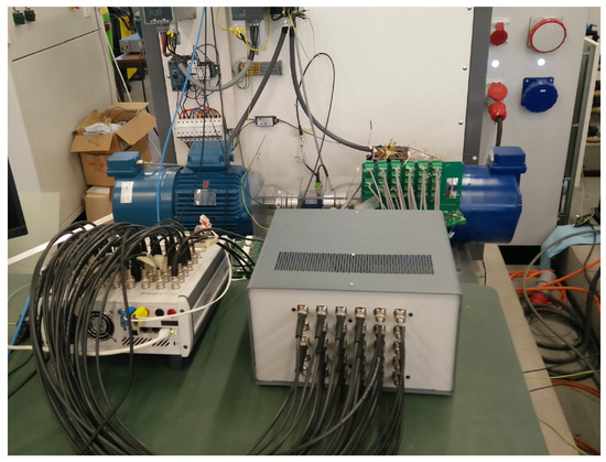
Figure 2.
Picture of the experimental test setup. The test induction motor (right) is mounted in back-to-back configuration with a induction motor (left) acting as a load emulator. Furthermore, the test motor is equipped with PT1000 RTDs in the stator and a contactless infrared temperature sensor is mounted close to the rotor end to measure its temperature.

Table 1.
Specifications of the induction motor and external fan.
The 3-phase stator currents of the test motor are measured with 3 Hall-effect LEM current transducers. Motor speed is measured with a standard 1024 incremental encoder from BEI Sensors, type DHO5 which is mounted on the shaft of the 7.5 kW load emulator. Furthermore, motor torque is measured with a torque sensor that is mounted in between the two motors with single lamellar couplings. The torque sensor is supplied by Lorenz Messtechnik GmbH, type DR-2112 and has a 50 Nm rating with an accuracy of ±0.05 Nm.
Platinum Resistance Temperature Detectors (RTDs) of type PT1000 have been embedded into the impregnated stator windings to measure its temperature. They have accuracy class A according to the DIN/IEC 60751 standard [31], which corresponds to an accuracy of with the measured temperature. Four-wire sensing is applied to eliminate any unwanted additional resistance increases due to heat-up of the sensing wires. Because of the high in the stator windings of the motor, the PT1000 temperature sensors are highly susceptible to high-frequency noise and DC offsets. An in-house designed multi-channel temperature board has been implemented to excite the PT1000s and filter out the high-frequency noise and DC offset on the measured signal, as well as condition the output signals for the data-acquisition through the MicroLabBox. The linearity error and common-mode rejection ratio of the temperature board have been measured to be 0.12% of full scale and −79.2 dB, respectively. The amplitude of the remaining noise is limited to 0.3 °C for the full measuring range.
The PT1000 temperature sensors are placed at different radial and axial positions inside the stator windings, as shown in Figure 3. The three relevant radial positions of the thermal sensors are located at the top, in the middle and at the bottom of the stator slot, respectively. In the axial position the sensors are placed equidistantly with a distance in between each sensor equivalent to a quarter length of the stator lamination pack. Sensors have also been placed in the end windings both at the drive side and the fan side, where three sensors are placed in each end winding: one close to the inner radius, a second in the middle and a third close to the outer radius of the end winding. In order to implement these sensors, the original impregnated stator windings were removed, and new stator windings were placed in the stator slots together with the PT1000 sensors. The stator windings were subsequently re-impregnated with a resin. Additional temperature sensors have also been placed in the stator tooth tip, stator tooth, yoke and on the motor frame to obtain a fully thermally instrumented induction motor. The 4 enameled copper wires of each temperature sensor exit the motor through the terminal box at the top and are connected to an intermediary board that is mounted on the side of the motor (cfr. Figure 2). Shielded cables connect each temperature sensor from the intermediary board to the corresponding input of the in-house designed multi-channel temperature board.
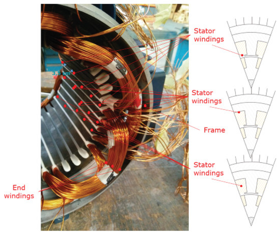
Figure 3.
Location of the PT1000 temperature sensors in the stator windings.
To measure the rotor temperature, a contactless infrared (IR) temperature sensor has been mounted close to the drive end of the rotor so that its field of view is entirely focused on the rotor surface. The IR sensor is supplied by Melexis and is of type MLX90614-ACC with an accuracy ranging from to .
Both motors are cooled independently with external ventilators mounted on each motor with the fan running at 2830 rpm. The fan specifications are listed in Table 1. Data-acquisition of all sensors and control of the test motor are performed simultaneously through the RTI of the MicroLabBox. Commanding setpoints of speed and torque are performed with the dSPACE ControlDesk 6.1 software.
In each of the measurement sets for model identification and for model validation, the 5.5 kW test induction motor is torque controlled, while the 7.5 kW is speed controlled. For each experiment, the motors are operated until thermal equilibrium is reached, while measuring both the stator temperatures and the rotor temperature.
4. Inverse Thermal Identification of the Induction Machine
An inverse methodology is used to determine the thermal parameter values of the LPTN (Section 2) starting from the experimental data collected on the fully thermally instrumented induction motor. Previous research has shown the identification of a steady-state higher-order LPTN (not consisting of capacitances) for a single motor operating point in [32]. A transient second-order LPTN was similarly identified in [24] with maximum estimation errors of only 4 °C for the stator windings, which was validated experimentally. However, no rotor temperature measurement or validation was presented in this work. A data-driven method was adopted in [20] to model the transient rotor temperature using subspace identification, which can be subsequently applied as an open-loop observer, but only the rotor temperature was considered here. As the accuracy of the modelled heat sources has a large impact on the modelled output temperatures, an investigation of the possibility of determining power losses in electrical machines based on the inverse identification methodology has been conducted in [21,22]. Finally, the results of an inverse identification of a LPTN for permanent magnet synchronous motors was presented, using a global identification technique for linear parameter-varying systems. The maximum estimation error is reported to be 8 °C. However, rigorous long-duration transient real-time thermal prediction of both stator and rotor of an induction motor, and accurate for the entire motor operating field ranging from zero to nominal speed and torque has yet to be investigated.
From the state-space system (2) there are 6 system parameters that need to be identified: the thermal resistances and , thermal capacitances and , and the heat sources and . As , and depend on the motor torque T and speed , the identification of these 6 parameters would only be valid for one specific motor operating point of speed and torque. To make sure that the thermal model is applicable for any T and , the 3 speed and torque dependent parameters need to be identified for multiple, well-chosen motor operating points . Three values for both T and have been selected ranging from zero to the nominal value in equal intervals, assuming that the motor predominantly operates in full nominal load and speed or lower loads and speed setpoints. This results in 9 combinations of the motor operating point , which means that the thermal system parameters need to be simultaneously fitted for 9 scenarios, where the motor operates at a fixed speed and torque T until thermal equilibrium is reached. As a result, 19 thermal system parameters need to be identified as specified in Table 2:
Table 2.
Thermal system parameters (Param) to be identified, relating to the values of the lumped parameters (Values) in (2).
This identification can be performed by aligning the modelled temperatures (11) with the measured temperature profiles using an iterative inverse methodology, as illustrated in Figure 4. The aim is to minimize the global cost function , which is proportional to the deviation between the modelled temperatures and the corresponding measured temperatures:
where and are the cost functions associated with the deviation of stator and rotor temperatures, respectively. and are the applied weight coefficients to both components. The stator and rotor cost component and both consist of on the one hand a cost associated with motor heating at certain operating points and on the other hand a cost associated with motor cooling at zero torque and speed:
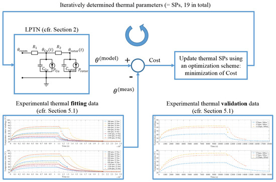
Figure 4.
Inverse methodology for the identification of the system thermal parameters.
The stator and rotor cost components corresponding to the heating phase and cooling phase can be expressed as:
where k denotes the time step according to the sampling time interval (here 3s) of the temperature measurements. The total time of the measured temperatures for the heating and cooling phase is approximately 3.5 h and 3 h, respectively.
The cost function (14) is minimized by updating the 19 thermal system parameters in Table 2 iteratively using an optimization scheme. A genetic algorithm with a population of 400 is used for this specific minimization problem. Elitism is set at 20 individuals that survive to each subsequent iteration. Furthermore, in each generation 80% of the remaining 380 individuals are created by crossover while the other 20% are created through mutation. This division ensures a good balance between local exploitation and global exploration in the searching algorithm. Crossover is performed by randomly selecting an individual whose coordinates are within the boundaries of the 19-dimensional hypercube formed by locating the parents at the opposite vertices:
where is a uniformly distributed random number between 0 and 1 (excluded). Mutation is performed by randomly selecting a direction that is adaptive to the last generation, as well as a step size, for the individual within the bounds and constraints.
The raw fitness scores of the individuals are scaled according to their rank r, with the fittest individual having , the second-fittest and so on. Fitness scaling converts the raw fitness score of the individuals into values that are adequate for the selection function, which uses these values to select the parents for the next generation. The scaled value of an individual with rank r is proportional to , which reduces the spread of the values with respect to the raw fitness values. A large spread of the fitness values used for selection would make the domination of the gene pool by the best individuals more likely, which would decrease the explorative behavior of the algorithm.
As , the following constraints were applied to the convection-dependent resistance :
Following the law for conservation of energy and power, the total motor power losses for a certain motor operating point can be determined from the difference between the electrical power input and the mechanical power output . The stator windings and rotor loss components are subjected to the following constraints, with :
where
where and are the measured DC voltage and current supplied to the motor, respectively. After identifying the 19 system parameters specified in Table 2, the 16 parameters that depend on T and are fitted to the functions (3)–(5). The resulting LPTN is validated using 3 additional sets of temperature measurements, each set corresponding to the motor operating at a fixed point where the motor heats up until thermal equilibrium is reached. The motor operating point of the 3 validation temperature sets are different from the 9 operating points of the data sets for identification of the LPTN.
5. Results and Discussion
This section details the results of the methodology and discussions are provided. First, we turn our attention to the collected measured data and zoom into the steady state and time constants of the measured temperature data sets. Secondly, the parameters within the LPTN are identified where the weighting factors in the cost function (14) are varied. Validation results of stator and rotor temperatures are subsequently presented both for static and intermittent loading. Finally, a sensitivity study is conducted of the different thermal system parameters on the stator/rotor temperature.
5.1. Steady State and Time Constants of the Measured Temperature Profiles
The measured average temperature of the stator windings and rotor for the 9 motor operating points used for model identification are shown in the upper and lower Figure 5, respectively. The average room temperature during measurements is . Steady-state temperatures are also listed in Table 3. Motor torque is varied in , while motor speed ranges in . As can be seen from Figure 5 and Table 3, the rotor temperature is consistently higher than the stator windings for all motor operating points, except for the first half hour where the opposite is true due to the higher thermal inertia of the rotor (and especially for the motor operating points at with higher thermal resistance ).
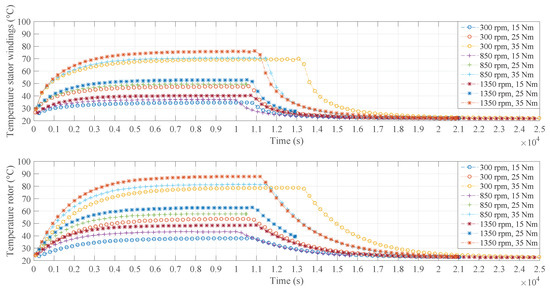
Figure 5.
Measured average temperature of the stator windings (upper figure) and the rotor (lower figure) for 9 motor operating points with motor torque setpoints and speed setpoints . When motor thermal equilibrium is reached, the motor is shut down and the temperatures in the cooling phase are measured. The average room temperature during measurements is , while temperature measurement sampling frequency is .
Table 3.
Average steady-state temperatures of the stator windings and the rotor at the 9 motor operating points for model identification.
The steady-state temperatures increase for higher motor speeds and higher torques T, both in the stator windings and the rotor. However, temperature changes are considerably more sensitive to changes in torque than in speed, as illustrated in Table 3. Transient thermal behavior can be quantified with a thermal time constant defined by the time needed for the temperature to reach :
where is the steady-state temperature and e is the Euler number. The experimentally determined thermal stator and rotor time constants and can be related to the eigenvalues and of the considered thermal model through the following expressions, by combining (11)–(13) and (27):
where , , and are determined coefficients that are dependent on , , , , , , and the initial conditions. Table 4 shows the time constants that are experimentally determined according to (27) for the model identification temperature data set. It is clear from Table 4 that the rotor time constant is considerably larger than the stator windings time constant for all operating points , which illustrates the larger thermal inertia of the rotor compared to the stator windings. Clear trends are visible as function of the motor speed : a higher consistently results in an increase of but a decrease of , for all motor operating points . For and , the rotor thermal time constant increases as function of motor torque T. No clear trend for at nor for is visible as function of T.
Table 4.
Time constants of the stator windings and the rotor at the 9 motor operating points for model identification.
Analogously, the temperature data set for model validation is generated and captured with the following motor operating points: . These operating points have been chosen to be fixed in between the operating points of the model identification temperature set. The transient temperatures are illustrated in Figure 6, while the steady-state temperatures and rotor time constants are presented in Table 5. From Figure 6 and Table 5 it can be seen that the rotor gets hotter than the stator windings for all three operating points. Furthermore, is consistently larger than as expected.
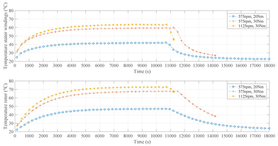
Figure 6.
Measured average temperature of the stator windings (upper figure) and the rotor (lower figure) for 3 motor operating points , and . When motor thermal equilibrium is reached, the motor is shut down and the temperatures in the cooling phase are measured. The average room temperature during measurements is , while temperature measurement sampling frequency is .
Table 5.
Steady-state temperatures and time constants of the stator windings and the rotor at the 3 motor operating points for model validation.
5.2. Thermal Model Parameter Identification
The identification of the thermal system parameters in Table 2 is performed by aligning the modelled temperatures with the corresponding measured temperatures using an iterative inverse methodology as explained in Section 4. The weight factors in (14) are chosen to be and respectively, giving stator and rotor temperatures equal importance of obtaining thermal alignment with the measurements. After convergence of the genetic algorithm, the solutions for the 19 SPs have been obtained (Table 6).
Table 6.
Identified thermal system parameters solution with equal weight of stator and rotor temperature in the cost function (14): and .
Table 7.
Fitting coefficients p for , and .
The modelled temperatures for are shown in Figure 7, where the upper figure shows the fitted temperature profile of the stator windings (blue) and the rotor (red) at , the middle figure at and the lower figure at .
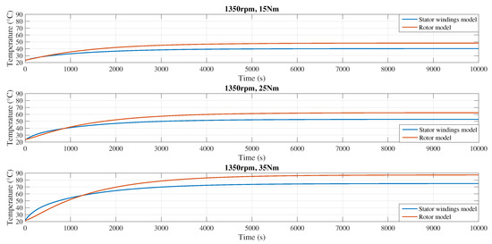
Figure 7.
Modelled temperature profiles of the stator windings (blue) and the rotor (red) for and (upper figure), (middle figure), (lower figure). Model identification with .
Figure 8 illustrates the thermal model error of the stator windings (blue) and the rotor temperature (red) for every time step, for the same 3 motor operating points considered above. It can be seen that the modelled temperature closely follows the measured temperature for both the stator windings and the rotor. The fitting errors are largest in the first hour of the transient regime for both the stator windings and the rotor, and subsequently converge to smaller error values as the temperatures get closer to reaching steady state. The modelled rotor temperature generally demonstrates larger fitting errors than the modelled average temperature of the stator windings. For the mean/max fitting errors for the stator windings and the rotor are and respectively, while for the mean/max fitting errors are and respectively. The rotor fitting errors are highest at : for the rotor mean/max fitting errors are and only for the stator.
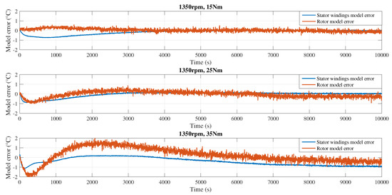
Figure 8.
Thermal model error of the stator windings (blue) and the rotor (red) temperature for and (upper figure), (middle figure), (lower figure). Model identification with .
Analogously, the mean and maximum thermal fitting errors of the identification data set for the remaining motor operating points are presented in Table 8 and Table 9 for the stator windings and the rotor, respectively. The mean rotor thermal fitting error is generally higher than the stator windings, while the maximum fitting error is consistently higher for the rotor than for the stator (except at ), especially at .
Table 8.
Mean and maximum modelling error of the stator windings temperature for 9 motor operating points . Solution of system parameters identified with different weighting factors in (14).
Table 9.
Mean and maximum modelling error of the rotor temperature for 9 motor operating points . Solution of system parameters identified with different weighting factors in (14).
In the cooling phase, the heat sources are absent and the rotor is at standstill: , and . The results of the thermal fitting of the cooling phase is shown in Figure 9, where the measured temperatures are well fitted within an error margin of .
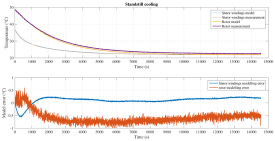
Figure 9.
Thermal model error of the stator windings and the rotor temperature for and . Model identification with .
As the modelling errors turn out to be higher for the rotor temperatures, a fitting can be performed for a higher rotor weight factor in the global cost function (14).
Table 10 shows the relative deviation of the system parameter solution with and from the solution obtained with equal weight factors . For higher the relative deviation of the identified system parameters also increases. In the newly identified set of system parameters the , and increase while , and decrease with respect to the initial solution. The largest deviations are seen for , and whereas and show the least system parameter variation.
Table 10.
Relative deviation (in %) of the identified system parameters from the values in Table 6 for two different sets of weight coefficients: .
Table 8 and Table 9 show the mean and maximal model fitting errors for different motor operating points of the stator and rotor temperatures, respectively, both for and . A higher value for the rotor weight consistently results in lower mean and maximal rotor temperature fitting errors, except for at , where the maximal rotor fitting error is only higher than for . The largest reduction in mean rotor temperature fitting error when increasing the rotor weight to occurs at , where the error is decreased by , and for , 850 and respectively. The corresponding maximal rotor fitting errors are decreased by , and , respectively. At and both the mean and maximal rotor fitting errors are reduced to less than half when changing from 1 to 6. However, this has a negative effect on the modelling accuracy of the stator temperatures, as is clear from Table 8. Increasing consequently increases the average stator temperature fitting errors for all motor operating points, except at where the average fitting error drops. The maximal stator fitting error at , however, increases by more than . The highest increase on average stator fitting error at occurs for with an increase of , and at , 25 and , respectively. The increase in maximal stator temperature fitting errors is the highest at , where an increase of , and are noted at , 850 and , respectively. These results suggest a trade-off between the accuracy of the stator and rotor temperature that are predicted with the considered second-order thermal model.
5.3. Model Validation
The temperature measurements of the stator windings and rotor at the 3 motor operating points , , are used for the validation of the experimentally identified thermal model. The results for are shown in Figure 10, Figure 11 and Figure 12, respectively. In these 3 figures, the upper figure illustrates the modelled and measured temperature of the stator windings and rotor, while the lower figure shows the absolute temperature error for the stator windings and the rotor. In contrast to the model identification results, the largest modelling errors in the validation results are situated in the steady-state regime instead of the transient regime. For the motor operating points and , the stator windings demonstrate the largest modelling error over the entire temperature profile compared to the rotor, with the exception of the first 15 min where the rotor modelling error is larger. At the modelling error of the rotor temperature is largest in the first 15 minutes, before it converges to approximately the same modelling error of the stator windings. The absolute mean and maximum error for both the stator windings and the rotor at the 3 motor operating points are listed in Table 11.
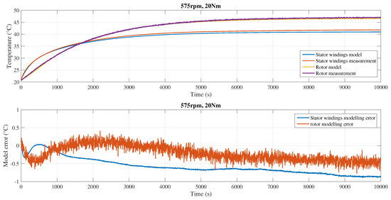
Figure 10.
Validation of the thermal model for with . Upper figure: modelled and measured temperature of the stator windings and the rotor. Lower figure: absolute modelling error for the stator windings and the rotor. The mean temperature errors for the stator windings and the rotor are and respectively, while the maximum errors are and .
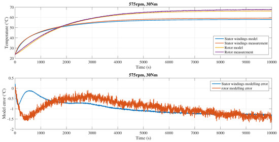
Figure 11.
Validation of the thermal model for with . Upper figure: modelled and measured temperature of the stator windings and the rotor. Lower figure: absolute modelling error for the stator windings and the rotor. The mean temperature errors for the stator windings and the rotor are and respectively, while the maximum errors are and .
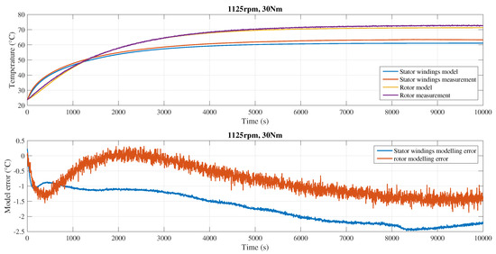
Figure 12.
Validation of the thermal model for with . Upper figure: modelled and measured temperature of the stator windings and the rotor. Lower figure: absolute modelling error for the stator windings and the rotor. The mean temperature errors for the stator windings and the rotor are and respectively, while the maximum errors are and .
Table 11.
Absolute mean and maximum thermal modelling errors for both the stator windings and the rotor, at 3 different motor operating points. Solution of system parameters identified with different weighting factors in [14].
For , the lowest average modelling error is achieved for the rotor temperature at with , whereas the highest average error is demonstrated for the stator windings at with . The highest maximum error is demonstrated for the stator windings, also at , with . The lowest maximum error can be found at for the rotor with . From Table 11 it can be seen that the proposed thermal model is able to predict the rotor temperature with higher accuracy compared to the stator windings, which is true for all values of . Furthermore, lower motor torque and speed setpoints generally result in higher thermal prediction accuracy, especially for the stator windings. Although a higher suggested a higher accuracy in rotor temperature prediction but a lower accuracy in stator temperature prediction in the previous section concerning the model fitting, this does not always seem true for the validation data set. While the average and maximal stator temperature errors are indeed mostly higher for compared to the case where , they are, however, generally lower for .
The transient behavior of the three thermal models corresponding to , and have also been tested on varying motor conditions where the motor torque is varied in discrete steps. The motor torque is varied between 10 and 30 Nm in stepwise fashion at different time instances to obtain an intermittent motor-loading regime, as shown in Figure 13. Motor speed is fixed at 1350 rpm for the entire duration of the intermittent loading test. Figure 14 and Figure 15 show the performance of the different thermal models for both the stator windings and rotor temperatures, respectively. From Figure 14 it can be seen that the thermal model performance for the stator windings is best for the solution corresponding with , followed by and , the last case resulting in the largest errors. The maximum stator temperature error for is while the average error is only . For the stator temperature errors are slightly higher with a maximum value of and a mean value of , while the largest stator temperature errors occur for with a maximum of and an average error of . The highest stator temperature errors generally occur in the first few minutes directly after a discrete change in motor operating point. However, the temperature errors never exceed , which is still better in terms of temperature accuracy compared to literature as discussed in the Introduction.
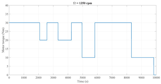
Figure 13.
Motor operating torque T variation during the intermittent load test for demonstrating the validity of the thermal transient performance of the thermal model. Motor speed remains constant at throughout the entire test.
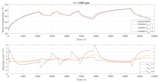
Figure 14.
Validation of the transient behavior of the thermal model for and stepwise changing motor torque setpoints. Upper figure: measured (blue) and modelled temperature of the stator windings for the model solution corresponding to (red), (yellow) and (purple). Lower figure: absolute stator windings temperature modelling error for the corresponding three model solutions.
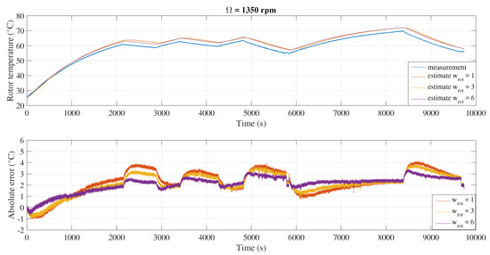
Figure 15.
Validation of the transient behavior of the thermal model for and stepwise changing motor torque setpoints. Upper figure: measured (blue) and modelled temperature of the rotor for the model solution corresponding to (red), (yellow) and (purple). Lower figure: absolute rotor temperature modelling error for the corresponding three model solutions.
Looking at Figure 15 for the rotor temperature estimation performance, the opposite trend can be seen for the model solutions with different values: in this case the best performance is obtained for , followed by and lastly the model solution corresponding to , which is to be expected according to the discussions in the previous paragraphs. The maximal and mean rotor temperature errors obtained for are and , respectively. For the maximal rotor temperature error is with an average error of , while for the obtained maximal and mean rotor temperature errors are and , respectively. The highest rotor temperature estimation errors occur right after the motor loading decreases to a lower load, in the regions where the rotor temperature cools down. However, this error consistently decreases to a lower value as time passes. To conclude, a clear trade-off can be observed between the accuracy of the stator and rotor temperature estimation for intermittent loading, especially in thermally transient operation: a higher stator temperature accuracy comes at a cost of a lower rotor temperature accuracy and vice versa. Depending on the priorities of the user, the corresponding model identification can be applied.
5.4. Sensitivity Study
A sensitivity study is conducted to investigate the effect of a change in one of the 6 system parameters in Table 2 on the temperature of the stator windings and the rotor. The 6 investigated parameters are , , , , and . The reference values for the SPs are selected as the solution obtained in Table 6 for the nominal motor operating point :
The resulting reference temperature profiles of the stator windings and rotor are shown as the dark blue curves (denoted by ‘Initial’ in the legend of the figure) in Figure 16 and Figure 17, respectively.
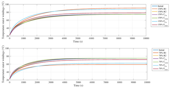
Figure 16.
Temperature sensitivity of the stator windings with respect to the 6 thermal SPs , , , , and . In the upper and lower figure, each profile represents the modelled temperature where one of the SPs is increased by or decreased by , respectively, while the other SPs retain their original values. The latter are obtained from the solution in Table 6 with .
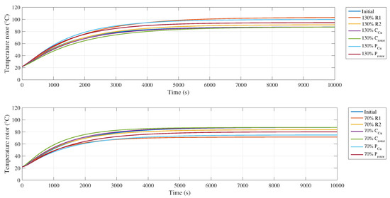
Figure 17.
Temperature sensitivity of the rotor with respect to the 6 thermal SPs , , , , and . In the upper and lower figure, each profile represents the modelled temperature where one of the SPs is increased by or decreased by , respectively, while the other SPs retain their original values. The latter are obtained from the solution in Table 6 with .
Each of the 6 parameters of Equation (30) is individually increased or decreased by a certain amount while the remaining 5 parameters retain their original reference values. The authors have chosen this amount to be 30 % of their reference parameter value indicated by (30), to have a clear effect on the stator and rotor temperature profiles. For example, to investigate the effect of , the stator and rotor temperature profiles are calculated once with (cfr. upper graphs of Figure 16 and Figure 17) and once with (cfr. lower graphs of Figure 16 and Figure 17), while the other parameters are unchanged, i.e., , , , and . The calculated stator temperatures and are then compared to , while the calculated rotor temperatures and are compared to . The effect of each of the 6 parameters on the temperature profiles of the stator windings and the rotor are presented in Figure 16 and Figure 17, respectively. Figure 16 shows that and have the largest effect on the temperature profile of the stator windings, especially on the steady-state regime. Furthermore, the temperature of the stator windings is the least sensitive to variations in the thermal resistance , for both the transient and steady-state regime. Notice that the deviation of temperature in the steady-state regime for a change in , or is symmetrical around the temperature of the reference case: an increase or decrease in either of these 3 SPs results in an increase or decrease by the same amount, respectively of the stator windings temperature.
The sensitivity of the thermal time constant and the steady-state temperature of the stator windings and the rotor are listed in Table 12 and Table 13, respectively.
Table 12.
Sensitivity of the thermal time constant and steady-state temperature of the stator windings with respect to the SPs.
Table 13.
Sensitivity of the thermal time constant and steady-state temperature of the rotor with respect to the SPs.
Table 12 shows that both and are most sensitive to the thermal resistance , while has the least effect on transient and steady-state regime. The thermal capacitances and are next in line for the sensitivity of , followed by and . The steady-state temperature is most sensitive to , followed by and , whereas , and simply do not have an effect on . Increasing , or results in higher and vice versa. An increase in , , or causes an increase in the thermal time constant , while a decrease in these SPs results in a decrease in with respect to the reference value. has the inverse effect on than the other SPs.
Figure 17 and Table 13 show that the behavior of the rotor temperature with respect to the SPs is more complex than the stator windings. The thermal resistance plays a larger role for both and as compared to the stator windings. Similar to the stator windings, has the largest effect for but only the second largest for . The thermal time constant is most sensitive to , followed by , , and lastly and . An increase in either of the 6 SPs except results in an increase in , while a decrease in these SPs causes a largely symmetrical decrease in with respect to the reference value. has an inverse effect on compared to the other 5 SPs.
The rotor steady-state temperature is most sensitive to , followed by , and . As expected, and do not have an effect on . An increase in , , or results in an increase of , while a decrease in one of these 4 SPs induces a symmetrical decrease in with respect to its reference value.
6. Conclusions
A methodology for the thermal condition monitoring of long-duration transient and steady-state temperatures in an induction motor has been presented. To achieve this goal, a computationally efficient second-order LPTN for a 5.5 kW squirrel-cage induction motor has been proposed to apprehend the dominant heat paths. This model has subsequently been identified through a data-driven, inverse approach and has been validated for a induction machine. The nodes of the thermal model represent the temperature of the stator windings and the rotor of the induction motor. The system parameters of the analytical thermal model have been identified by aligning the modelled temperatures of the stator windings and the rotor with the measured temperatures for different, fixed motor operating points and their subsequent zero-operation cooling temperature profiles. This is performed iteratively using a genetic algorithm to minimize a cost function that is proportional to the cumulative deviation of the modelled temperature with respect to the corresponding measured temperature. A test induction motor has been equipped with thermal contact sensors to measure the stator windings at different locations, as well as a contactless infrared sensor to measure the rotor temperature. The test motor is independently cooled with an external fan. In total, 12 thermal measurement data sets have been obtained through measurement, where each data set corresponds to the measured temperature of both the stator windings and the rotor while the motor is running at a certain fixed speed and torque until thermal equilibrium is reached. The motor is subsequently shut off and the cooling curve is measured. Nine thermal data sets have been obtained for model identification, where motor torque and speed vary according to and , respectively. The remaining three data sets are used for model validation and correspond to fixed motor operating points located in between those of the data sets used for model identification: . Varying the weight factors that indicate the relative importance of the stator and rotor temperature in the cost function to be minimized, results in different thermal parameter solution sets with a higher temperature prediction accuracy for either the stator or the rotor temperature depending on the cost function weight factors. Validation results show that during motor operation at fixed speed and torque, the absolute average thermal modelling error of the stator windings and the rotor for the selected weight factors do not exceed and , respectively, while the maximal absolute error of the stator windings and the rotor is limited to and , respectively. In intermittent motor loading it is shown that for the stator windings temperature an average modelling error of can be achieved with a maximal error of , while for the rotor temperature a mean and maximal error of and can be obtained, respectively. These results show the validity of the proposed thermal model, and can be used to predict in real time the temperature of the stator windings and the rotor for condition monitoring or motor control.
Author Contributions
All the work and writing are primarily carried out by P.N.P. Conceptualization P.N.P., K.S. and G.C.; methodology, P.N.P. and G.C.; hardware resources, H.V. and D.B.; writing—review and editing by all authors equally; supervision, K.S. and G.C. All authors have read and agreed to the published version of the manuscript.
Funding
This research was supported by the MoForM project of Flanders Make, the strategic research centre for the manufacturing industry of Flanders, Belgium. This research also received funding from the Flemish Government under the ’Onderzoeksprogramma Artificiële Intelligentie (AI) Vlaanderen’ programme.
Conflicts of Interest
The authors declare no conflict of interest.
Appendix A. Explicit Solution of the 2nd Order Thermal Model
To obtain the explicit solution for , the Laplace transformation is applied to the system (6). After rearranging, the Laplace transform of the temperature vector can be written as:
with a unity matrix, the initial conditions of and the Laplace transform of the input vector . The first and second part correspond to the Laplace transform of the zero-input response and zero-state response, respectively:
The eigenvalues and of the state-space system are calculated by solving the characteristic polynomial for the complex variable s:
The solution of the second order equation in s is written as:
Assuming that , , and , it can be proven that both and , which translates into an exponentially stable behaviour of the temperature states. The inverse of is calculated as:
with and as calculated in (A4). Decomposition of (A5) with partial fractions results in:
with
Assuming that the input vector is constant, its Laplace transform can be written as:
References
- Boglietti, A.; Cavagnino, A.; Staton, D.; Shanel, M.; Mueller, M.; Mejuto, C. Evolution and Modern Approaches for Thermal Analysis of Electrical Machines. IEEE Trans. Ind. Electron. 2009, 56, 871–882. [Google Scholar] [CrossRef]
- Nikbakhsh, A.; Izadfar, H.R.; Jazaeri, M. Classification and comparison of rotor temperature estimation methods of squirrel cage induction motors. Measurement 2019, 145, 779–802. [Google Scholar] [CrossRef]
- Zidani, F.; Diallo, D.; Benbouzid, M.E.H.; Nait-Said, R. Direct torque control of induction motor with fuzzy stator resistance adaptation. IEEE Trans. Energy Convers. 2006, 21, 619–621. [Google Scholar] [CrossRef]
- Nguyen Phuc, P.; Vansompel, H.; Bozalakov, D.; Stockman, K.; Crevecoeur, G. Data-Driven Online Temperature Compensation for Robust Field-Oriented Torque Controlled Induction Machines. IET Electr. Power Appl. 2019, 13, 1954–1963. [Google Scholar] [CrossRef]
- Huai, Y.; Melnik, R.V.; Thogersen, P.B. Computational analysis of temperature rise phenomena in electric induction motors. Appl. Therm. Eng. 2003, 23, 779–795. [Google Scholar] [CrossRef]
- Liu, X.; Yu, H.; Shi, Z.; Xia, T.; Hu, M. Electromagnetic-fluid-thermal field calculation and analysis of a permanent magnet linear motor. Appl. Therm. Eng. 2018, 129, 802–811. [Google Scholar] [CrossRef]
- Melka, B.; Smolka, J.; Hetmanczyk, J.; Bulinski, Z.; Makiela, D.; Ryfa, A. Experimentally validated numerical model of thermal and flow processes within the permanent magnet brushless direct current motor. Int. J. Therm. Sci. 2018, 130, 406–415. [Google Scholar] [CrossRef]
- Mellor, P.H.; Roberts, D.; Turner, D.R. Lumped parameter thermal model for electrical machines of TEFC design. IEE Proc. B Electr. Power Appl. 1991, 138, 205–218. [Google Scholar] [CrossRef]
- Nerg, J.; Rilla, M.; Pyrhonen, J. Thermal Analysis of Radial-Flux Electrical Machines With a High Power Density. IEEE Trans. Ind. Electron. 2008, 55, 3543–3554. [Google Scholar] [CrossRef]
- Valenzuela, M.A.; Reyes, P. Simple and Reliable Model for the Thermal Protection of Variable-Speed Self-Ventilated Induction Motor Drives. IEEE Trans. Ind. Appl. 2010, 46, 770–778. [Google Scholar] [CrossRef]
- Wallscheid, O.; Böcker, J. Global Identification of a Low-Order Lumped-Parameter Thermal Network for Permanent Magnet Synchronous Motors. IEEE Trans. Energy Convers. 2016, 31, 354–365. [Google Scholar] [CrossRef]
- Boglietti, A.; Cossale, M.; Vaschetto, S.; Dutra, T. Winding Thermal Model for Short-Time Transient: Experimental Validation in Operative Conditions. IEEE Trans. Ind. Appl. 2018, 54, 1312–1319. [Google Scholar] [CrossRef]
- Dorrell, D.G. Combined Thermal and Electromagnetic Analysis of Permanent-Magnet and Induction Machines to Aid Calculation. IEEE Trans. Ind. Electron. 2008, 55, 3566–3574. [Google Scholar] [CrossRef]
- Nategh, S.; Zhang, H.; Wallmark, O.; Boglietti, A.; Nassen, T.; Bazant, M. Transient Thermal Modeling and Analysis of Railway Traction Motors. IEEE Trans. Ind. Electron. 2019, 66, 79–89. [Google Scholar] [CrossRef]
- Boglietti, A.; Cavagnino, A.; Staton, D. Determination of Critical Parameters in Electrical Machine Thermal Models. IEEE Trans. Ind. Appl. 2008, 44, 1150–1159. [Google Scholar] [CrossRef]
- Howey, D.A.; Childs, P.R.N.; Holmes, A.S. Air-Gap Convection in Rotating Electrical Machines. IEEE Trans. Ind. Electron. 2012, 59, 1367–1375. [Google Scholar] [CrossRef]
- Boglietti, A.; Cavagnino, A.; Lazzari, M.; Pastorelli, M. A simplified thermal model for variable-speed self-cooled industrial induction motor. IEEE Trans. Ind. Appl. 2003, 39, 945–952. [Google Scholar] [CrossRef]
- Ahmed, F.; Kar, N.C. Analysis of End-Winding Thermal Effects in a Totally Enclosed Fan-Cooled Induction Motor With a Die Cast Copper Rotor. IEEE Trans. Ind. Appl. 2017, 53, 3098–3109. [Google Scholar] [CrossRef]
- Kim, C.; Lee, K.S. Thermal nexus model for the thermal characteristic analysis of an open-type air-cooled induction motor. Appl. Therm. Eng. 2017, 112, 1108–1116. [Google Scholar] [CrossRef]
- Zaiser, S.; Buchholz, M.; Dietmayer, K. Rotor Temperature Modeling of an Induction Motor using Subspace Identification. IFAC-PapersOnLine 2015, 48, 847–852. [Google Scholar] [CrossRef]
- Nair, D.G.; Arkkio, A. Inverse Thermal Modeling to Determine Power Losses in Induction Motor. IEEE Trans. Magnet. 2017, 53, 1–4. [Google Scholar] [CrossRef]
- Nair, D.G.; Rasilo, P.; Arkkio, A. Sensitivity Analysis of Inverse Thermal Modeling to Determine Power Losses in Electrical Machines. IEEE Trans. Magnet. 2018, 54, 1–5. [Google Scholar] [CrossRef]
- Orlande, H.R.B. Inverse Problems in Heat Transfer: New Trends on Solution Methodologies and Applications. J. Heat Transf. 2012, 134, 031011. [Google Scholar] [CrossRef]
- Zhang, P.; Du, Y.; Habetler, T.G. A Transfer-Function-Based Thermal Model Reduction Study for Induction Machine Thermal Overload Protective Relays. IEEE Trans. Ind. Appl. 2010, 46, 1919–1926. [Google Scholar] [CrossRef]
- Phuc, P.N.; Stockman, K.; Crevecoeur, G. Inverse Methodology for the Parameter Identification of a Lumped Parameter Thermal Network for an Induction Machine. In Proceedings of the 2018 International Symposium on Power Electronics, Electrical Drives, Automation and Motion (SPEEDAM), Amalfi, Italy, 20–22 June 2018; pp. 298–303. [Google Scholar] [CrossRef]
- De Morais Sousa, K.; Hafner, A.A.; Carati, E.G.; Kalinowski, H.J.; da Silva, J.C.C. Validation of thermal and electrical model for induction motors using fiber Bragg gratings. Measurement 2013, 46, 1781–1790. [Google Scholar] [CrossRef]
- Li, K.; Wang, S.; Sullivan, J.P. A novel thermal network for the maximum temperature-rise of hollow cylinder. Appl. Therm. Eng. 2013, 52, 198–208. [Google Scholar] [CrossRef]
- Boglietti, A.; Carpaneto, E.; Cossale, M.; Vaschetto, S. Stator-Winding Thermal Models for Short-Time Thermal Transients: Definition and Validation. IEEE Trans. Ind. Electron. 2016, 63, 2713–2721. [Google Scholar] [CrossRef]
- Yahoui, H.; Grellet, G. Measurement of physical signals in rotating part of electrical machine by means of optical fibre transmission. In Proceedings of the Quality Measurement: The Indispensable Bridge between Theory and Reality (No Measurements? No Science! Joint Conference—1996: IEEE Instrumentation and Measurement Technology Conference and IMEKO Technical Committee 7), Brussels, Belgium, 4–6 June 1996; Volume 1, pp. 591–596. [Google Scholar] [CrossRef]
- Ganchev, M.; Kubicek, B.; Kappeler, H. Rotor temperature monitoring system. In Proceedings of the XIX International Conference on Electrical Machines—ICEM 2010, Rome, Italy, 6–8 September 2010; pp. 1–5. [Google Scholar] [CrossRef]
- IEC 60751: Industrial Platinum Resistance Thermometers and Platinum Temperature Sensors; International Electrotechnical Commission: Geneva, Switzerland, 2008.
- Bousbaine, A.; McCormick, M.; Low, W.F. In-situ determination of thermal coefficients for electrical machines. IEEE Trans. Energy Convers. 1995, 10, 385–391. [Google Scholar] [CrossRef]


© 2019 by the authors. Licensee MDPI, Basel, Switzerland. This article is an open access article distributed under the terms and conditions of the Creative Commons Attribution (CC BY) license (http://creativecommons.org/licenses/by/4.0/).