Computational Study of Flow and Heat Transfer Characteristics of EG-Si₃N₄ Nanofluid in Laminar Flow in a Pipe in Forced Convection Regime ^†

Abstract

Laminar flow of ethylene glycol-based silicon nitride (EG-Si₃N₄) nanofluid in a smooth horizontal pipe subjected to forced heat convection with constant wall heat flux is computationally modeled and analyzed. Heat transfer is evaluated in terms of Nusselt number (Nu) and heat transfer coefficient for various volume fractions of Si₃N₄ nanoparticles in the base fluid and different laminar flow rates. The thermophysical properties of the EG-Si₃N₄ nanofluid are taken from a recently published experimental study. Computational modelling and simulation are performed using open-source software utilizing finite volume numerical methodology. The nanofluid exhibits non-Newtonian rheology and it is modelled as a homogeneous single-phase mixture, the properties of which are determined by the nanoparticle volume fraction. The existing features of the software to simulate single-phase flow are extended by implementing the energy transport coupled to the fluid flow and the interaction of the fluid flow with the surrounding pipe wall via the applied wall heat flux. In addition, the functional dependencies of the thermophysical properties of the nanofluid on the volume fraction of nanoparticles are implemented in the software, while the non-Newtonian rheological behavior of the nanofluid under consideration is also taken into account. The obtained results from the numerical simulations show very good predicting capabilities of the implemented computational model for the laminar flow coupled to the forced convection heat transfer. Moreover, the analysis of the computational results for the nanofluid reflects the increase of heat transfer of the EG-Si₃N₄ nanofluid in comparison to the EG for all the considered nanoparticle volume fractions and flow rates, indicating promising features of this nanofluid in heat transfer applications.

1. Introduction

Nanofluids are mixtures or suspensions of small particles of order of tens of nanometer in pure base fluids, which after mixing and dispersing the nanoparticles have shown the potential to increase heat transfer in engineering applications. The increase in thermal conductivity of nanofluids relative to the base fluid was first time indicated by Choi and Eastman [1]. They conducted a theoretical study of thermal conductivity of nanofluids with copper nanophase materials. Consequently, due to their discovered potential in a variety of applications incorporating heat transfer, such as heat exchangers, solar collectors, or thermal energy storage systems, the research in nanofluids has been intensified over the past years [2,3,4,5,6]. For the base fluids water and ethylene glycol are commonly used in both, the experimental [5,7,8,9,10,11,12,13,14] and the numerical studies [4,15,16,17]. The numerical investigation has been directed towards two main different approaches by modeling the nanofluid flow either as an effective single-phase mixture with unique properties depending on the nanoparticle volume fraction, or a two-phase flow with explicitly accounting for the interaction of the nanoparticles with the base fluid [18]. In the last several years ionic liquids (ILs) have been used more and more as base fluids for producing the nanofluids [19,20,21,22,23,24,25]. At ambient conditions ionic liquids have the property of being non-volatile and non-flammable and they are recyclable liquids. These are the reasons why ionic liquids are very often considered as green fluids. By suspending nanoparticles in an ionic liquid, the so called ionanofluid (INF) is formed. Ionanofluids is a new type of nanofluids which can further increase the thermophysical properties of ionic liquids. In a recent study [26] the available research and results are summarized in order to assess the potential of ionanofluids. In spite of scattering of the literature results, it was concluded that ionanofluids have good potential in advanced thermal and energy applications. The recently conducted researches especially point at ionanofluids as potential media for advanced solar collectors [19,20,21,22,23,24,25].

In addition to the convincing results for the enhancement of the heat transfer a broader approach to research in nanofluids has to identify the drawback of their usage, such as the obvious problem of sedimentation of the nanoparticles after a long-time storage [27,28,29], or even the costs that have to be paid for the increased efficiency in the energy performance [30], since the enhancement in heat transfer characteristics might not be enough to balance the increase the pressure drop in terms of costs.

The materials of nanoparticles used for forming the nanofluids are commonly oxides, metals, carbides, and carbon nanotubes. In the last several years suspensions of nitride nanoparticles in base fluids have been started to be used for research [9,10,11,12,13,31,32,33,34,35]. Promising results have been obtained so far which point out that thermal conductivity enhances with the volume fraction of nanoparticles in suspension. The increase of the thermal conductivity for hexagonal boron nitride nanofluids (average particle size 70 nm) goes up to 26% at volume fractions of 3% for water and up to and 16% for the same volume fraction in EG-based nanofluids [10]. The research of thermophysical properties of EG-based nanofluids with TiN nanoparticles has been conducted for average nanoparticle diameters of 30 nm and 50 nm and nanoparticle volume fraction from 0.0022 to 0.0111. It was concluded that thermal conductivity of considered nanofluids could be improved by decreasing the size of nanoparticles [13]. Contrary to that, the thermal conductivity of nanofluids with boron nitride (BN) nanoparticles in ethylene glycol was found to be possible to be enhanced with increasing the nanoparticle size [9]. The main reason for this was concluded to be the surface area and the aspect ratio of BN nanoparticles. In the same study one more abnormality related to thermal conductivity enhancements of BN/EG nanofluids is noticed. The higher increase of the thermal conductivity was achieved at a low nanoparticle volume fraction. The authors suspect the chain-like loose aggregation of nanoparticles to be the reason for this uncommon increase of thermal conductivity at very low volume fraction of nanoparticles. Nanofluids with suspended aluminum nitride nanoparticles (AlN) in ethylene glycol (average particle sizes 165 nm) and propylene glycol (average particle sizes 169 nm) as base fluids with the nanoparticle volume fraction of 0.1 increase the thermal conductivity by 38.71% and 40.2%, respectively [31]. Computational fluid dynamics using the finite-volume method and adopting the SIMPLE algorithm was performed for flowing of suspension of aluminum nitride nanoparticles (particle size 30 nm) in ethylene glycol as the base fluid through a horizontal heated tube [32]. Overall efficiency of heat transfer enhancement was above one for ranges of nanoparticle concentrations from 1% to 3% and Reynolds numbers from zero to 20,000. The heat capacity of nanofluids with ethylene glycol and three different types of nitride nanoparticles (namely, aluminum nitride AlN, silicon nitride Si₃N₄, and titanium nitride (TiN) was experimentally determined in [33]. It was concluded that the volume fraction of nanoparticles has a strong effect on the heat capacity, whereas the nanoparticle size does not show a significant impact on this thermophysical property.

The findings presented above nominate nanofluids with suspended nitrides for in-depth research in the future. In numerical simulations nanofluid is often modelled as a single-phase Newtonian fluid, which is considered to be a good balance between the achieved numerical accuracy and the acceptable computational costs, in particular for use in practical engineering applications, which may be accompanied by flows in complex geometries or involve some additional complex physics. However, in the available literature there is a lack in studies of nanofluids which exhibit some more complex rheology. The present study focuses on computational modelling and analysis of a laminar flow of a non-Newtonian nanofluid (ethylene glycol-based silicon nitride (EG-Si₃N₄)) in a horizontal pipe with respect to the forced convection heat transfer.

The nanofluid considered in the present study is ethylene glycol-based silicon nitride, which was experimentally examined in [35] by measuring its rheological behavior and thermal properties in addition to the electrical conductivity and optical properties, all as functions of the concentration of nanoparticles. In the above-mentioned experimental study, the average size of the nanoparticles is 20 nm and the suspension was produced in a production method using vortex shaker, ultrasonic bath, and high-energy ultrasound generator. The properties of the nanofluid are determined for volume fractions of nanoparticles up to 0.035. The obtained experimental results reveal the non-Newtonian shear thinning behavior of the nanofluid, a simple linear increase of thermal conductivity with volume fraction of nanoparticles, as well as a high enhancement of electrical conductivity and an increase of optical properties (refractive index, absorption) with volumetric concentration of nanoparticles. Such behavior of the properties renders the EG-Si₃N₄ nanofluid as being convenient not only in applications for heat transfer, such as heat exchangers and thermal energy storage, but also for applications where enhanced electrical and optical properties are of importance, such as electromagnetic flow meters or solar collectors.

The present computational study is devoted to determining the heat transfer characteristics of the EG-Si₃N₄ nanofluid when it is subjected to laminar pipe flow and forced convection heat transfer with a constant wall heat flux. Heat transfer is evaluated by determining the Nusselt number and the heat transfer coefficient for various volume fractions of Si₃N₄ nanoparticles at different nanofluid flow rates. The computational model is implemented in the open-source software foam-extend ver. 4.0 [36], which represents an extension of the widely used open-source software OpenFOAM^® [37] utilizing finite volume numerical methodology. The results show that the heat transfer of the EG-Si₃N₄ nanofluid increases in comparison with the ethylene glycol as the base fluid.

2. Computational Model

2.1. Governing Transport Equations and Constitutive Relations

The nanofluid considered here is modeled as a single-phase mixture with thermophysical properties depending on the nanoparticle volume fraction. The computational model for the steady-state flow of such a fluid is given by the governing equations for the mass, linear momentum, and energy conservation with neglected temperature induced density changes:

$$\nabla \cdot \left(\rho \mathit{U}\right)=0,$$

(1)

$$\nabla \cdot \left(\rho \mathit{U}\mathit{U}\right)=-\nabla p+\nabla \cdot \tau ,$$

(2)

$$\nabla \cdot \left(\rho c_p\mathit{U}T\right)=\nabla \cdot \left(k\nabla T\right),$$

(3)

where ρ is the density of the nanofluid, U is the velocity, p is the pressure, τ is the viscous stress tensor, c_p is the specific heat, k is the thermal conductivity, and T is the temperature. The changes in density due to temperature changes in the fluid are neglected since the effects of the natural heat convection are not considered. This is a consequence of the assumption that the effects of the forced heat convection are predominant in comparison to the natural heat convection. This assumption is justified for cases where the flow is constrained to small geometries, such as the one used here (tube with 4 mm inner diameter), whereas the natural heat convection effects become important in larger geometries [38].

To evaluate the density and the specific heat of the nanofluid, weighted averages based on the volume fraction of nanoparticles are use, according to the expressions:

$$\rho ={\phi }_v{\rho }_n+\left(1-{\phi }_v\right){\rho }_{bf},$$

(4)

$$\rho c_p={\phi }_v{\left(\rho c_p\right)}_n+\left(1-{\phi }_v\right){\left(\rho c_p\right)}_{bf},$$

(5)

where φ_v is the volume fraction of nanoparticles in the suspension and the indices n and bf refer to nanoparticles and base fluid, respectively.

The thermal conductivity of the EG-Si₃N₄ nanofluid is modelled as a linear dependency on the nanoparticle volume fraction, with the expressions [35]:

$$k=\left(1+2.87{\phi }_v\right)k_{bf}.$$

(6)

The rheology of the EG-Si₃N₄ nanofluid is modelled with the expressions [35]:

$$\tau ={\tau }_0+K{\gamma }^n,$$

(7)

where γ represents the strain rate, while the parameters τ₀, K, and n depend on the Si₃N₄ nanoparticle volume fraction φ_v and their values are provided in [35]. The Expression (7) represents the Herschel-Bulkley rheology model, which is implemented in the software foam-extend in a manner that avoids the numerical stability problems for very low values of the strain rate and the singularity at the limiting case of γ = 0, which would mathematically correspond to infinite viscosity. The local viscous stress tensor can be represented as the product of the local nanofluid dynamic viscosity μ and the local strain rate $\gamma$, corresponding to the given local viscous stress. If the dynamic viscosity is expressed in terms of the kinematic viscosity, the local viscous stress is $\tau =\rho \nu \gamma$ and the Equation (2) can be rewritten in the following form:

$$\nabla \cdot \left(\mathit{U}\mathit{U}\right)=-\frac{1}{\rho }\nabla p+\frac{1}{\rho }\nabla \cdot \tau =-\frac{1}{\rho }\nabla p+\frac{1}{\rho }\nabla \cdot \left(\mu \gamma \right)=-\frac{1}{\rho }\nabla p+\frac{1}{\rho }\nabla \cdot \left(\rho \nu \gamma \right).$$

(8)

The kinematic viscosity is determined from the expression:

$$\nu =\frac{1}{\rho }\frac{\tau }{\gamma }=\frac{1}{\rho }\frac{{\tau }_0+K\left[{\gamma }^n-{\left(\frac{{\tau }_0}{{\nu }_0}\right)}^n\right]}{\dot{\gamma }}=\frac{1}{\rho }\frac{{\tau }_0+K\left({\gamma }^n-{\gamma }_0^n\right)}{\gamma },$$

(9)

where the small value for the strain rate ${\gamma }_0={\tau }_0/{\nu }_0$ is introduced in order to be able to control the situation of very small local strain rates during the computation. Thus, the viscous stress is evaluated from the expression:

$$\tau ={\tau }_0+K\left({\gamma }^n-{\gamma }_0^n\right),$$

(10)

and the graphical representation is given in Figure 1. The value for γ₀ is determined by setting the viscosity ν₀ to some high value (say 0.1), as the input parameter to the model. The value for the viscosity, which is required in the momentum equation, is then determined as being equal to ν₀ for local values of γ < γ₀ and the viscous stress is then closely equal to τ₀, whereas for γ > γ₀ the viscous stress calculated from the expression (10) will nearly be equal to the theoretical value in the expression (7). In this manner, the singularity at γ = γ₀ is avoided and the numerically obtained viscous stress is negligibly different from the theoretical value in the expression (7), the difference being determined by the value for ν₀ and γ₀: the higher the value for ν₀ is set, the lower will be the value for γ₀ and the viscous stress will be closer to the theoretical value.

2.2. Geomery Modeling and Numerical Mesh

The geometry consists of a smooth horizontal pipe in which the flow is axisymmetric due to the assumption of negligible effects of natural heat convection. Therefore, in order to significantly reduce the computational efforts, the pipe can be modelled as a 2-D axisymmetric slice and the numerical mesh is two-dimensional having only one cell in the azimuthal direction, as shown in Figure 2.

2.3. Discretization of Transport Equations and Boundary Conditions

For the discretization of various terms in the governing transport equations the finite-volume numerical methodology is used. The numerical mesh is made of a number of small volumes (cells), in which each two cells share one flat cell-face. All variables are stored at cell-centroids (cell-centers) denoted with P and all cells are bounded by a finite number of flat cell-faces denoted with f. The transport equations representing conservation laws in a steady state simulation may be written in a generic form for some variable ϕ:

$$\nabla \cdot \left(\rho \mathit{U}\varphi \right)=\nabla \cdot \left(\Gamma \nabla \varphi \right)+S_{\varphi }\left(\varphi \right),$$

(11)

where ϕ stands for one in the continuity equation, for U in the momentum equation and for T in the energy equation, Γ is the diffusion coefficient, replaced by ν in the momentum equation and by k/c_p in the energy equation, and S_ϕ represent any sources which may be present and depend on ϕ. There is no such source in the present model in the energy equation, so the only term treated as a source of momentum is the negative pressure gradient in the momentum equation. All terms in Equation (11) are discretized within the finite-volume approximation and the transport equations are integrated over all cell-volumes:

$${\displaystyle \underset{V_P}{\int }\nabla \cdot \left(\rho \mathit{U}\varphi \right)\mathrm{d}V}={\displaystyle \underset{V_P}{\int }\nabla \cdot \left(\Gamma \nabla \varphi \right)\mathrm{d}V}+{\displaystyle \underset{V_P}{\int }{S}_{\varphi }\left(\varphi \right)\mathrm{d}V}$$

(12)

The discretization of terms containing spatial derivatives is performed by converting the volume integrals in surface integrals according to Gauss’s theorem and then summing over all cell-faces f is performed. The gradient-containing terms are approximated according to the expression:

$${\displaystyle \underset{V_P}{\int }\nabla \varphi \mathrm{d}V}={\displaystyle \underset{S_P}{\int }\varphi \mathrm{d}\mathit{S}}\approx {\displaystyle \sum _f{\mathit{S}}_f}{\varphi }_f.$$

(13)

where S_P is the surface area of all the cell-faces enclosing the control volume V_P, S_f is the surface of a cell-face, and dS is the differential of the cell-face surface-normal vector. The summation is again done over all cell-faces f bounding a cell P. In accordance, divergence-containing terms are discretized as:

$${\displaystyle \underset{V_P}{\int }\nabla \cdot \varphi \mathrm{d}V}={\displaystyle \underset{S_P}{\int }\varphi \cdot \mathrm{d}\mathit{S}}\approx {\displaystyle \sum _f{\mathit{S}}_f\cdot }{\varphi }_f$$

(14)

Similarly, the second-order spatial terms are approximated as:

$${\displaystyle \underset{V_P}{\int }\nabla \cdot \left(\Gamma \nabla \varphi \right)\mathrm{d}V}={\displaystyle \underset{S_P}{\int }\mathrm{d}\mathit{S}\cdot \left(\Gamma \nabla \varphi \right)}\approx {\displaystyle \sum _f{\Gamma }_f{\mathit{S}}_f\cdot \left(\nabla {\varphi }_f\right)}.$$

(15)

For the calculation of surface integrals, the unknown variables are interpolated to the centers of the cell-faces. The approximation of the terms with gradients does not impose severe restrictions, so that simple linear interpolation can be used, while on the other hand the discretization of the term involving the divergence, in particular the convective term in the momentum equation, is more problematic and approximation of the convective term represents one of the challenges in Computational Fluid Dynamics (CFD). Due to the simplicity of the problem studied a simple upwind convection scheme is considered to be sufficient here for the convective terms in both, the momentum and the energy equations. In the momentum equation the convective term is linearized by calculating the volume flux through the cell-faces from the previous iteration.

In approximations of source terms, the corresponding values at cell-centers are reconstructed from the values at the cell-faces. For example, the source containing the pressure gradient is calculated according to the expression:

$${\left(\nabla p\right)}_P\approx {\left({\displaystyle \sum _f\frac{{\mathit{S}}_f{\mathit{S}}_f}{\left|{\mathit{S}}_f\right|}}\right)}^{-1}\cdot \left({\displaystyle \sum _f\frac{{\mathit{S}}_f}{\left|{\mathit{S}}_f\right|}}\cdot \left(\nabla p_f^{\perp }\right)\left|{\mathit{S}}_f\right|\right),$$

(16)

where the symbol ⊥ denotes the surface-normal gradient, which is obtained by a simple linear scheme between two neighboring computational cells.

For solving the coupled flow and heat transfer problem described by transport Equations (1)–(3) and the constitutive relations (4)–(10), boundary conditions are prescribed at domain boundaries (pipe inlet, pipe outlet, and pipe wall, with reference to Figure 2). The boundary conditions are summarized in the following.

Momentum:

• inlet: U = (U_in, 0, 0), ∇p = 0,
• pipe wall: U = (0, 0, 0), ∇p = 0,
• outlet: ∇U = 0, p = p_out.

Energy:

• inlet: T = T_in,
• pipe wall: ∇T = q/k, where q is the applied wall heat flux,
• outlet: $\nabla T=qD\mathsf{\pi }/\left(\dot{m}{c}_p\right)$,

where D is the inner diameter of the pipe and $\dot{m}$ is the mass flow rate. Thus, for the momentum, there is an inflow boundary at the inlet of the pipe with the prescribed uniform velocity and an outflow boundary at the outlet of the pipe. As for the energy, a uniform temperature is prescribed at the inlet, while the temperature gradient is imposed at the pipe wall which is obtained from the given heat flux. At the outlet, the temperature gradient is imposed which is evaluated theoretically from the analytical solution $\nabla T=qD\mathsf{\pi }/\left(\dot{m}{c}_p\right)$ valid for a constant wall heat flux [39].

Upon the discretization, sets of linear algebraic equations are obtained for each unknown variable, each set of algebraic equations representing a counterpart of the corresponding transport equation:

$$a_P{\varphi }_P+{\displaystyle \sum _N{a}_N{\varphi }_N=b},$$

(17)

where the summation is performed over all the neighboring cells N surrounding the cell P of interest and the term b on the right-hand side represents the explicit terms.

The linear systems of algebraic equations are solved to obtain the numerical approximate solutions of the governing transport equations. The system of Equation (17) is solved in an iterative solution procedure, starting from an initial estimate and continually improving the solution in every iteration. The iteration loop is stopped, and the solution is reached when the difference between the solutions in two consecutive iterations is smaller than some small prescribed tolerance.

The proper coupling between the pressure and the velocity in the momentum equation is ensured by using the continuity equation to derive the discrete form of the pressure equation from the discrete form of the momentum equation and iterate via the SIMPLE algorithm for steady-state flows, as implemented in OpenFOAM^® [40], which is extended to iterate over the energy equation as well:

• Set all fields to initial values.
• Assemble and solve the under-relaxed momentum equation (momentum predictor).
• Assemble and solve the pressure equation and calculate the conservative volume fluxes, then update the pressure field with under-relaxation and correct the velocity explicitly.
• Solve the temperature equation using the available volume fluxes, pressure and velocity fields; under-relax the equation implicitly in order to improve convergence.
• Check convergence for all equations; if the system is not converged, start a new iteration from the step 2.

3. Results

The described computational model is implemented in the foam-extend version of the software OpenFOAM^®. The capabilities of the model are first verified by computing a single-phase flow with heat transfer and comparing the computationally obtained results with the existing results in the available literature. After that, the model is used to compute the nanofluid flow and obtain results for various volume fractions of the nanoparticles in the mixture.

For the purpose of evaluation of the heat transfer characteristics, the local Nusselt number and heat transfer coefficient are calculated along the pipe axial axis, as well as the average heat transfer coefficient. The mean temperature of the fluid in a pipe cross-section S is evaluated from the following expression:

$$T_m=\frac{{\displaystyle \underset{S}{\int }\rho c_{p}T\mathit{U}\cdot \mathrm{d}\mathit{S}}}{{\displaystyle \underset{S}{\int }\rho c_p\mathit{U}\cdot \mathrm{d}\mathit{S}}},$$

(18)

The local heat transfer coefficient and the Nusselt number in the pipe cross-section are evaluated from the following expressions:

$$h=\frac{-k\nabla T_{wall}}{T_{wall}-T_m},$$

(19)

$$Nu=\frac{hD}{k},$$

(20)

and the average heat transfer coefficients for the pipe is evaluated from the following expression:

$$\overline{h}=\frac{1}{L}{\displaystyle \underset{0}{\overset{L}{\int }}h\mathrm{d}x}$$

(21)

In the above expressions the indices m and wall refer to mean value and value at the pipe wall, respectively, D is the diameter and L is the length of the pipe, and overbar denotes the average value. The local values for T_m, h and Nu are calculated for each column of cells along the axial axis of the pipe. Thus, the number of calculated values in the direction of the axial pipe axis is equal to the number of cells in the axial direction.

For the evaluation of the flow hydrodynamics, the friction factor for laminar flow in the pipe is calculated from the expression:

$$f=\frac{-2\nabla pD}{\rho {\overline{v}}^2}$$

(22)

where $\overline{v}$ is the mean flow velocity in the pipe cross-section, which is equal to the inlet velocity, and ∇p is the local pressure gradient in the same cross-section.

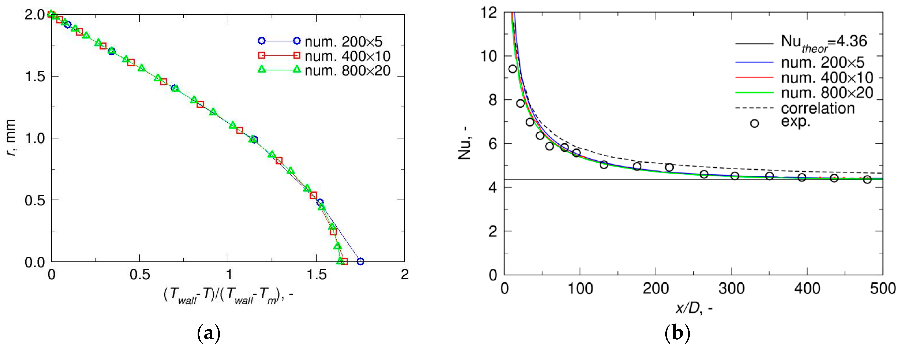
3.1. Verification of the Computational Model

The model is verified for a pure fluid, without nanoparticles, against the known analytical solution [39], the experimental results [38], and the empirical result [41]. In the computational setup, the pipe geometry and fluid (water) properties are the same as in [38], with the Reynolds number of the flow Re = 965, the wall heat flux q = 1000 W/m² and the temperature of the fluid at the inlet is T_in = 293 K, as listed in

Table 1. Parameters in the computational setup used for the verification.

Pipe Diameter D	Pipe Length L	Inlet Temperature Tin	Wall Heat Flux q	Reynolds Number Re
4 mm	5 m	293 K	1000 W/m2	965

. The fluid in these simulations is Newtonian and the viscous stress tensor is calculated as $\tau =\mu \left[\nabla \mathit{U}+{\left(\nabla \mathit{U}\right)}^T\right]$, instead of using the Herschel-Bulkley model. There meshes were used for the verification: 200 × 5, 400 × 10 and 800 × 20 cells in the axial and radial directions, respectively. Figure 3 shows the computationally obtained velocity profile and the friction factor for the laminar flow of water. The results for both, the velocity profile and the friction factor, converge with increasing mesh resolution.

The model predicts very accurately the analytical parabolic velocity profile and the theoretical friction factor, which in this case is f = 64/Re = 0.0663, except at the entrance into the pipe where the boundary layer still develops.

The computed local Nusselt number and the dimensionless radial temperature profile in the pipe cross-section are plotted in Figure 4. The computationally obtained results converge with decreasing the mesh size in both, the dimensionless radial temperature distribution and the Nusselt number. The analytical solution for the Nusselt number Nu = 4.36 is also correctly evaluated and the computational results for the Nusselt number are in very good agreement with the experimental results in [38] and also the empirical result from [41].

In order to have an impression on the distributions (fields) of the velocity and the temperature in the pipe, these distributions are shown in Figure 5 for the velocity, and in Figure 6 for the temperature. Due to the large length-to-diameter ratio of the pipe, only results for the parts of the pipe at its inlet and outlet are shown. It can clearly be seen how the velocity and temperature boundary layers develop from the pipe entrance to the pipe outlet. At the pipe outlet the velocity boundary layer is fully developed, while the temperature boundary layer still seems to develop. This is expected, since the hydrodynamic entry length is estimated as (x_h/D) ≈ 0.05Re and the thermal entry length is estimated as (x_t/D) ≈ 0.05RePr [39], where Pr is the Prandtl number. Thus, for the Prandtl number Pr > 1, as is the case here, the velocity boundary layer develops faster than the thermal boundary layer. This is also the reason why the boundary condition for the energy equation at the pipe outlet is given in terms of the gradient of the temperature, which can be calculated analytically and is not a function of the axial coordinate of the pipe [39].

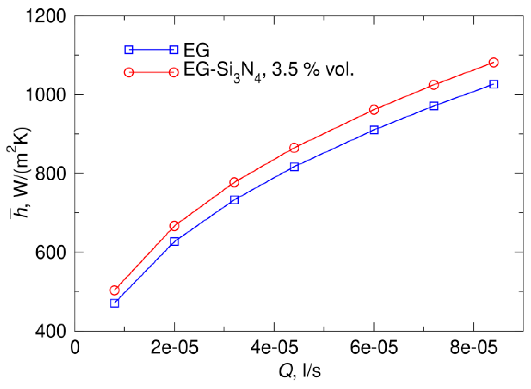
3.2. Results for the EG-Si₃N₄ Nanofluid

After the verification of the computational model in regard to the flow dynamics and heat transfer, further computations of the laminar flow of the EG-Si₃N₄ nanofluid are done. The pipe in the following simulations has a length of 2 m and a diameter of 4 mm, and the applied wall heat flux is equal to 10 kW/m². According to the previous results of the verification, and noting that the pipe length is smaller in the simulations with the nanofluid, the numerical mesh consisting of 400 × 20 cells is taken as sufficient for the simulations. Simulations are performed for various volume flow rates and nanoparticle volume fractions, according to

Table 2. Parameters used for the simulation scenarios for ethylene glycol-based silicon nitride (EG-Si₃N₄) nanofluid.

Pipe Diameter D	Pipe Length L	Inlet Temperature Tin	Wall Heat Flux q	Volume Flow Rate Q	Nanoparticle Volume Fraction φv
4 mm	2 m	293 K	10 kW/m2	8 × 10−6–8.4 × 10−5 m3/s	0–0.035

.

In Table 2 the volume flow rates of the nanofluid from Q = 8 × 10⁻⁶ to 8.4 × 10⁻⁵ m³/s, which were used in the simulations, correspond to the Reynolds numbers in the range from Re = 200 to Re = 2100 expressed for the base fluid (pure EG). The thermophysical properties for the pure EG as the base fluid and the Si₃N₄ nanoparticles are listed in

Table 3. Thermophysical properties of the base fluid (EG).

Density ρ	Specific Heat cp	Heat Conductivity k
1109.67 kg/m3	2458.3 J/(kg K)	0.2429 W/(m K)

and

Table 4. Thermophysical properties of nanoparticles (Si₃N₄).

Density ρ	Specific Heat cp	Heat Conductivity k
3400 kg/m3	540 J/(kg K)	16.7 W/(m K)

, respectively.

Figure 7 shows the computationally obtained velocity profile of EG as base fluid and of EG-Si₃N₄ with nanoparticle volume fraction of 3.5% for the volume flow rate Q = 6 × 10⁻⁵ m³/s, which corresponds to Re = 1500 for the base fluid. The results reflect the difference in the computed velocity profiles, in particular around the symmetry axis of the pipe, where the profile obtained with the non-Newtonian rheology becomes flattened as expected. It can be concluded that the non-Newtonian shear thinning rheology is correctly predicted by the computational model.

The computed heat transfer coefficients of EG as base fluid and of EG-Si₃N₄ with different nanoparticle volume fractions are plotted in Figure 8 for the volume flow rates Q = 8 × 10⁻⁶ m³/s, which corresponds to Re = 200 for EG, and for Q = 6 × 10⁻⁵ m³/s, which corresponds to Re = 1500 for EG. It can be observed that the heat transfer coefficient in the nanofluid is higher than the one in the pure base fluid, and the increase of the volume fraction of the nanoparticles leads to the increase of the heat transfer coefficient.

Furthermore, simulations were performed with the highest volume fraction of the nanoparticle of ϕ_v = 3.5% in a range of Reynolds numbers between 200 and 2100 (which correspond to the pure EG) and the results for the average heat transfer coefficient in the pipe are shown in Figure 9. As can be seen, the increase in the volume flow rate leads to the increase in the heat transfer coefficient, and the increase of the heat transfer coefficient is slightly more pronounced at higher flow rates.

Finally, the computational results for the relative enhancement of the average heat transfer coefficient for the EG-Si₃N₄ nanofluid at the volume fraction of nanoparticles of 3.5% over a range of nanofluid volume flow rates corresponding to Re between 200 and 2100 for pure EG are shown in Figure 10. The relative enhancement of the average heat transfer coefficient is higher at lower flow rates and amounts to 6.5% at the lowest flow rate, while the enhancement is slightly decreasing at higher flow rates. This is attributed to the fact that at higher flow rates the heat transfer coefficient of the pure base fluid is also increased, which slightly damps the relative enhancement.

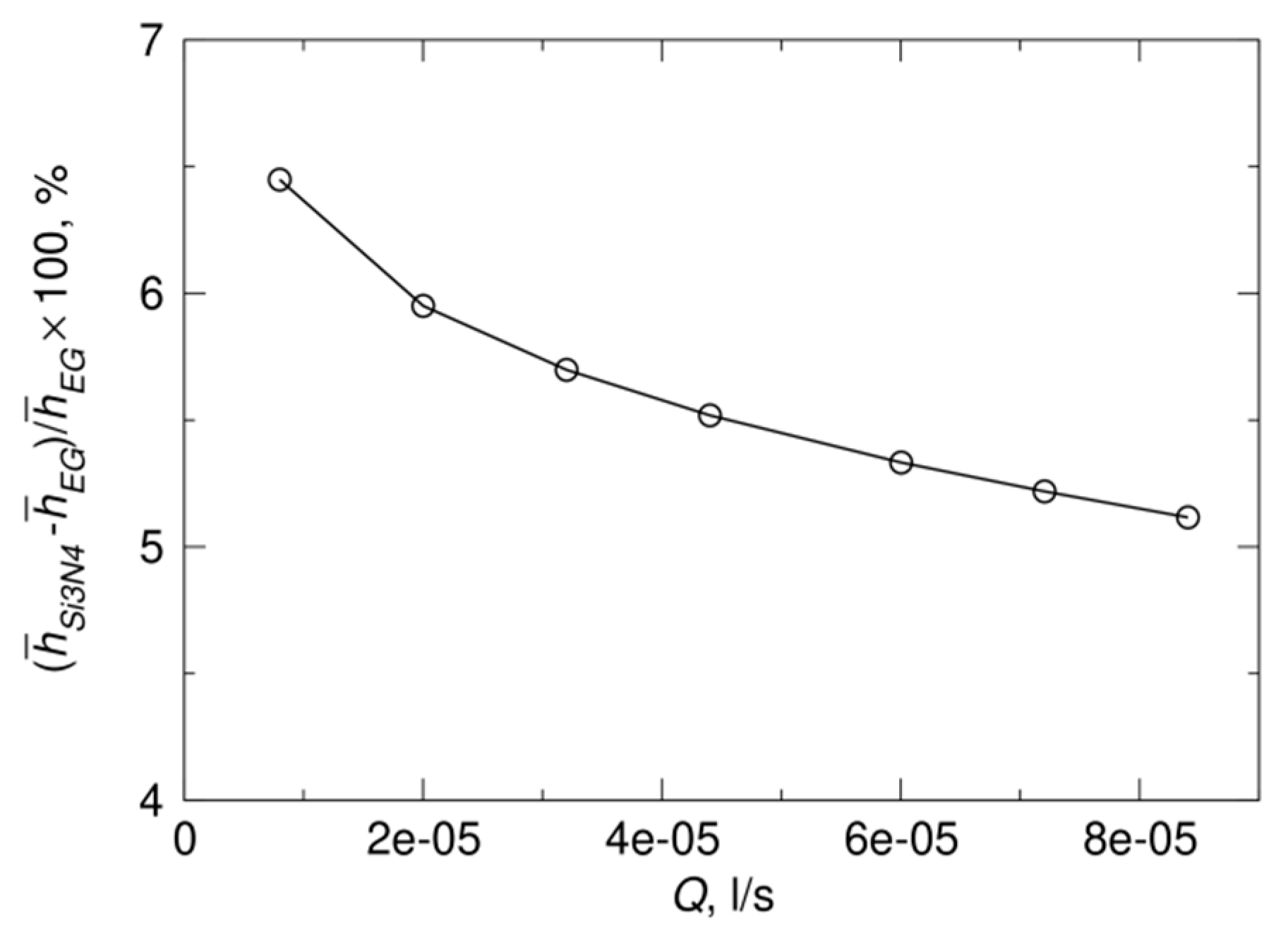
3.3. Discussion on the Performance Evaluation

The heat transfer enhancement alone should not be used as the only criterion for the evaluation of the heat transfer performance of the nanofluid compared to the pure base fluid. The increase of the viscosity of the nanofluid should also be taken into account, in particular in cases where the change in the viscosity leads to the change in the rheology of the nanofluid. The benefit of using the nanofluid for the heat transfer enhancement in engineering should be estimated bearing in mind the additional pumping power required to compensate for the loss of flow performance due to the increase of the viscosity. Different approaches are proposed in the literature as criteria for the thermal performance evaluation of nanofluids [19,42,43,44]. They are basically all somehow related to the consideration of the heat transfer performance of the nanofluid compared with the base fluid and relative to the loss of flow power. However, the criteria are proposed by different authors for the specific configuration under consideration (type of the nanofluid, geometry and wall boundary condition) and it seems not to be possible to find a unique criterion straightforwardly. It is therefore advisable to use a criterion which is as simple as possible, while containing information about the relation of the heat transfer increase and the power loss in the nanofluid flow. Since the heat transfer enhancement is directly proportional to the enhancement in thermal conductivity and the loss of the flow power is proportional to the increase in the viscosity, one such criterion for the performance evaluation of the nanofluid is the simple comparison of ratios of thermal conductivities and viscosity of the nanofluid and the base fluid:

$$\frac{k_{nf}}{k_{bf}}>{\left(\frac{{\mu }_{nf}}{{\mu }_{bf}}\right)}^{1/3},$$

(23)

where the indices nf and bf refer to nanofluid and base fluid, respectively. This criterion can be derived by requiring that the difference between the wall and bulk fluid temperature in the nanofluid flow should be smaller than the one in the flow of the base fluid. It follows from expression (23) that that the specific nanofluid could be considered to be beneficial for use if the nanofluid-to-base fluid thermal conductivity ratio is greater than the third root of the nanofluid-to-base fluid viscosity ratio in the laminar flow regime.

This simple criterion is tested in the present study for various nanoparticle volume fractions and the results are listed in

Table 5. Performance evaluation of the EG-Si₃N₄ nanofluid.

Nanoparticle Volume Fraction φv	Thermal Conductivity Ratio knf/kbf	Viscosity Ratio (μnf/μbf)1/3
0.0	1	1
0.0033	1.00947	1.04483
0.0066	1.01894	1.05741
0.01	1.02870	1.07655
0.0134	1.03846	1.11588
0.0169	1.04850	1.13608
0.0258	1.07404	1.24519
0.035	1.100450	1.44602

. The values for the thermal conductivity ratio and the one-third power of the viscosity ratio are relatively close, but the criterion is not satisfied. According to this performance evaluation criterion it would be questionable whether the nanofluid used in the present study would be considered as beneficial for heat transfer applications. In other words, in addition to the gain in the heat transfer performance of the nanofluid, it is important to account for the additional power loss which is in the same order of magnitude but has slightly higher value than the gain in heat transfer.

4. Conclusions

Heat transfer characteristics in laminar flow of the EG-Si₃N₄ nanofluid in a pipe with the imposed constant wall heat flux have been numerically analyzed. The computational model incorporating coupled fluid flow and energy transport has been implemented in the finite-volume numerical approach to enable simulations in the framework of CFD. The nanofluid is modeled as a single-phase mixture, the properties of which are determined based on the volume fraction of nanoparticles. In contrast to most previous studies, the rheology of the nanofluid also depends on the nanoparticle volume fraction and the non-Newtonian shear thinning nanofluid rheology has been taken into account. The model is verified by computing laminar pipe flow coupled with a constant wall heat flux and comparing the numerical results with the available experimental, empirical, and analytical results. The computational model is then used to compute the pipe flow of the EG-Si₃N₄ nanofluid subjected to constant wall heat flux and forced heat convection. Simulated scenarios include various flow rates and nanoparticle volume fractions in the laminar flow regime. The obtained results show that the heat transfer coefficient in the flow of the nanofluid is higher than the one corresponding to the base fluid for the same flow rates, the heat transfer coefficient increases with increasing the volume fraction of nanoparticles and the heat transfer coefficient also increases with increasing the flow rate. The relative enhancement of the average heat transfer coefficient in all cases is higher than 5% and it is about 6.5% at lower flow rates. Although the obtained heat transfer enhancement might appear as lower than expected, this enhancement is still achieved with the EG-Si₃N₄ nanofluid, while on the other hand it is important to note that this nanofluid was recently also found to have very enhanced electrical and optical properties. Thus, it may be considered as suitable for engineering applications where, in addition to the heat transfer, enhanced electrical and optical properties are also important. Furthermore, the present study shows that a relatively simple computational model with the nanofluid being treated as a single-phase mixture offers a convenient and reliable tool for the analysis of nanofluid flow and heat transfer by means of CFD. Finally, it is emphasized that, in spite of the proven capability of the nanofluid to enhance the heat transfer characteristics, it is always very important to objectively asses the performance of the nanofluid in terms of the power loss due to the increase of the viscosity by estimating the nanofluid performance according to an appropriate performance evaluation criterion.

References

1. Choi, S.U.; Eastman, J.A. Enhancing Thermal Conductivity of Fluids with Nanoparticles; Technical report, TRN: 96:001707; Argonne National Laboratory: Argonne, IL, USA, 1995.
2. Bianco, V.; Manca, O.; Nardini, S.; Vafai, K. Heat Transfer Enhancement with Nanofluids, 1st ed.; CRC Press: Boca Raton, FL, USA, 2017; pp. 207–287. [Google Scholar]
3. Huminic, G.; Huminic, A. Application of nanofluids in heat exchangers: A review. Renew Sustain. Energy Rev. 2012, 16, 5625–5638. [Google Scholar] [CrossRef]
4. Boukerma, K.; Kadja, M. Convective Heat Transfer of Al2O3 and CuO Nanofluids Using Various Mixtures of Water-Ethylene Glycol as Base Fluids. Eng. Technol. Appl. Sci. Res. 2017, 7, 1496–1503. [Google Scholar]
5. Madhesh, D.; Kalaiselvam, S. Experimental study on the heat transfer and flow properties of Ag–ethylene glycol nanofluid as a coolant. Heat Mass Transf. 2014, 50, 1597–1607. [Google Scholar] [CrossRef]
6. Wong, K.V.; De Leon, O. Applications of Nanofluids: Current and Future. Adv. Mech. Eng. 2010, 2, 1–11. [Google Scholar] [CrossRef] [Green Version]
7. Bhanvase, B.A.; Sarode, M.R.; Putterwar, L.A.; Abdullah, K.A.; Deosarkar, M.P.; Sonawane, S.H. Intensification of convective heat transfer in water/ethylene glycol based nanofluids containing TiO2 nanoparticles. Chem. Eng. Process. 2014, 82, 123–131. [Google Scholar] [CrossRef]
8. Sundar, L.S.; Singh, M.K.; Sousa, A.C.M. Enhanced heat transfer and friction factor of MWCNT–Fe3O4/water hybrid nanofluids. Int. Commun. Heat Mass Transf. 2014, 52, 73–83. [Google Scholar] [CrossRef]
9. Li, Y.; Zhou, J.; Luo, Z.; Tung, S.; Schneider, E.; Wu, J.; Li, X. Investigation on two abnormal phenomena about thermal conductivity enhancement of BN/EG nanofluids. Nanoscale Res. Lett. 2011, 6, 1–7. [Google Scholar] [CrossRef] [Green Version]
10. Ilhan, B.; Kurt, M.; Ertürk, H. Experimental investigation of heat transfer enhancement and viscosity change of hBN nanofluids. Exp. Therm. Fluid Sci. 2016, 77, 272–283. [Google Scholar] [CrossRef]
11. Zyła, G.; Fal, J.; Traciak, J.; Gizowska, M.; Perkowski, K. Huge thermal conductivity enhancement in boron nitride–ethylene glycol nanofluids. Mater. Chem. Phys. 2016, 180, 250–255. [Google Scholar] [CrossRef]
12. Zyła, G.; Fal, J. Experimental studies on viscosity, thermal and electrical conductivity of aluminum nitride–ethylene glycol (AlN–EG) nanofluids. Thermochim. Acta 2016, 637, 11–16. [Google Scholar] [CrossRef]
13. Zyła, G.; Fal, J.; Estellé, P. Thermophysical and dielectric profiles of ethylene glycol based titanium nitride (TiN–EG) nanofluids with various size of particles. Int. J. Heat Mass Transf. 2017, 113, 1189–1199. [Google Scholar] [CrossRef]
14. Sarafraz, M.M.; Safaei, M.R.; Tian, Z.; Goodarzi, M.; Filho, E.P.B.; Arjomandi, M. Thermal Assessment of Nano-Particulate Graphene-Water/Ethylene Glycol (WEG 60:40) Nano-Suspension in a Compact Heat Exchanger. Energies 2019, 12, 1929. [Google Scholar] [CrossRef] [Green Version]
15. Akbari, M.; Galanis, N.; Behzadmehr, A. Comparative analysis of single and two-phase models for CFD studies of nanofluid heat transfer. Int. J. Therm. Sci. 2011, 50, 1343–1354. [Google Scholar] [CrossRef]
16. Ravnik, J.; Škerget, L.; Yeigh, B.W. Nanofluid natural convection around a cylinder by BEM. WIT Trans. Model. Sim. 2015, 61, 261–271. [Google Scholar]
17. Ravnik, J.; Škerget, L. Simulation of flow of nanofluids by BEM. WIT Trans. Model. Sim. 2010, 50, 3–14. [Google Scholar]
18. Minea, A.A.; Buonomo, B.; Burggraf, J.; Ercole, D.; Karpaiya, K.R.; Di Pasqua, A.; Sekrani, G.; Steffens, J.; Tibaut, J.; Wichmann, N.; et al. NanoRound: A benchmark study on the numerical approach in nanofluids’ simulation. Int. Commun. Heat Mass Transf. 2019, 108, 104292. [Google Scholar] [CrossRef]
19. Titan, C.P.; Morshed, A.K.M.M.; Khan, J.A. Nanoparticle enhanced ionic liquids (NEILS) as working fluid for the next generation solar collector. Procedia Eng. 2013, 56, 631–636. [Google Scholar]
20. Bhattacharjee, A.; Luís, A.; Santos, J.H.; Lopes-da-Silva, J.A.; Freire, M.G.; Carvalhoa, P.J.; Coutinho, J.A.P. Thermophysical properties of sulfonium- and ammonium-based ionic liquids. Fluid Phase Equilib 2014, 381, 36–45. [Google Scholar] [CrossRef] [Green Version]
21. Titan, P.C.; Morshed, A.K.M.M.; Fox, E.B.; Visser, A.N.; Bridges, N.J.; Khan, J.A. Thermal performance of ionic liquids for solar thermal applications. Exp. Therm. Fluid Sci. 2014, 59, 88–95. [Google Scholar]
22. Titan, P.C.; Morshed, A.K.M.M.; Fox, E.B.; Khan, J.A. Effect of nanoparticle dispersion on thermophysical properties of ionic liquids for its potential application in solar collector. Procedia Eng. 2014, 90, 643–648. [Google Scholar]
23. Titan, P.C.; Morshed, A.K.M.M.; Fox, E.B.; Khan, J.A. Thermal performance of Al2O3 Nanoparticle Enhanced Ionic Liquids (NEILs) for Concentrated Solar Power (CSP) applications. Int. J. Heat Mass Transf. 2015, 85, 585–594. [Google Scholar]
24. Titan, P.C.; Morshed, A.K.M.M.; Fox, E.B.; Khan, J.A. Enhanced thermophysical properties of NEILs as heat transfer fluids for solar thermal applications. Appl. Therm. Eng. 2017, 110, 1–9. [Google Scholar]
25. Chereches, E.I.; Sharma, K.V.; Minea, A.A. A numerical approach in describing ionanofluids behavior in laminar and turbulent flow. Contin. Mech. Thermodyn. 2018, 30, 657–666. [Google Scholar] [CrossRef]
26. Minea, A.A.; Sohel Murshed, S.M. A review on development of ionic liquid based nanofluids and their heat transfer behavior. Renew Sustain Energy Rev. 2018, 91, 584–599. [Google Scholar] [CrossRef]
27. Mukherjee, S.; Paria, S. Preparation and Stability of Nanofluids-A Review. IOSR-JMCE 2013, 9, 63–69. [Google Scholar] [CrossRef]
28. Sharma, B.S.K.; Gupta, S.M. Preparation and evaluation of stable nanofluids for heat transfer application: A review. Exp. Therm. Fluid Sci 2016, 79, 202–212. [Google Scholar]
29. Zhao, M.; Lv, W.; Li, Y.; Dai, C.; Zhou, H.; Song, X.; Wu, Y. A Study on Preparation and Stabilizing Mechanism of Hydrophobic Silica Nanofluids. Materials 2018, 11, 1385. [Google Scholar] [CrossRef] [Green Version]
30. Alirezaie, A.; Hajmohammad, M.H.; Alipour, A.; Salari, M. Do nanofluids affect the future of heat transfer? A benchmark study on the efficiency of nanofluids. Energy 2018, 157, 979–989. [Google Scholar] [CrossRef]
31. Yu, W.; Xie, H.; Li, Y.; Chen, L. Experimental investigation on thermal conductivity and viscosity of aluminum nitride nanofluid. Particuology 2011, 9, 187–191. [Google Scholar] [CrossRef]
32. Hussein, A.M.; Noor, M.M.; Kadirgama, K.; Ramasamy, D. Heat transfer enhancement using hybrid nanoparticles in ethylene glycol through a horizontal heated tube. Int. J. Automot. Mech. Eng. 2017, 14, 4183–4419. [Google Scholar] [CrossRef]
33. Zyła, G.; Vallejo, J.P.; Lugo, L. Isobaric heat capacity and density of ethylene glycol based nanofluids containing various nitride nanoparticle types: An experimental study. J. Mol. Liq. 2018, 261, 530–539. [Google Scholar] [CrossRef]
34. Abbasi, F.M.; Gul, M.; Shehzad, S.A. Hall effects on peristalsis of boron nitride-ethylene glycol nanofluid with temperature dependent thermal conductivity. Physica E 2018, 99, 275–284. [Google Scholar] [CrossRef]
35. Zyla, G.; Fal, J.; Bikić, S.; Wanic, M. Ethylene glycol-based silicon nitride nanofluids: An experimental study on their thermophysical, electrical and optical properties. Physica E 2018, 104, 82–90. [Google Scholar] [CrossRef]
36. Wikki Consultancy and Software Developement Using Foam-Extend and OpenFOAM®. Available online: http://wikki.gridcore.se/foam-extend (accessed on 24 September 2019).
37. OpenFOAM The Open-Source CFD Toolbox. Available online: https://www.openfoam.com/ (accessed on 24 September 2019).
38. Meyer, J.P.; Everts, M. Single-phase mixed convection of developing and fully developed flow in smooth horizontal circular tubes in the laminar and transitional flow regimes. Int. J. Heat Mass Transf. 2018, 117, 1251–1273. [Google Scholar] [CrossRef] [Green Version]
39. Bergman, T.L.; Lavine, A.S.; Incropera, F.P.; Dewitt, D.P. Fundamentals of Heat and Mass Transf., 7th ed.; John Wiley & Sons Inc.: Hoboken, NJ, USA, 2011; pp. 518–558. [Google Scholar]
40. Jasak, H. Error Analysis and Estimation for the Finite Volume Method with Applications to Fluid Flows. Ph.D. Thesis, Imperial College of Science, Technology and Medicine, London, UK, June 1996. [Google Scholar]
41. Shah, R.K.; London, A.L. Laminar Flow Forced Convection in Ducts, 1st ed.; Academic Press: New York, NY, USA, 1978; pp. 78–138. [Google Scholar]
42. Prasher, R.; Song, D.; Wang, J.; Phelan, P. Measurements of nanofluid viscosity and its implications for thermal applications. Appl. Phys. Lett. 2006, 89, 133108. [Google Scholar] [CrossRef]
43. Wu, Z.; Feng, Z.; Sundén, B.; Wadsö, L. A comparative study on thermal conductivity and rheology properties of alumina and multi-walled carbon nanotube nanofluids. Front. Heat Mass Transf. 2014, 5, 1–10. [Google Scholar]
44. Sekrani, G.; Poncet, S.; Proulx, P. Modelling of convective turbulent heat transfer of water-based Al2O3 nanofluids in a uniformly heated pipe. Chem. Eng. Sci. 2018, 176, 205–219. [Google Scholar] [CrossRef]
Figure 1. Herschel-Bulkley model for non-Newtonian fluid rheology.
Energies 13 00074 g001
Figure 2. Geometry and mesh modeling: (a) 2-D axisymmetric domain flow; (b) Snapshot of the 2-D numerical mesh.
Energies 13 00074 g002
Figure 3. Results for laminar flow of water at Re = 965: (a) The computed velocity profile evaluated at x/D = 625; (b) The computed friction factor.
Energies 13 00074 g003
Figure 4. Results for laminar flow of water at Re = 965: (a) The computed dimensionless temperature profile evaluated at x/D = 625; (b) The computed Nusselt number.
Energies 13 00074 g004
Figure 5. The computed velocity distribution (expressed in m/s) for laminar flow of water at Re = 965: (a) Inlet part of the pipe; (b) Outlet part of the pipe.
Energies 13 00074 g005
Figure 6. The computed temperature distribution (expressed in K) for laminar flow of water at Re = 965: (a) Inlet part of the pipe; (b) Outlet part of the pipe.
Energies 13 00074 g006
Figure 7. The computed velocity profile for laminar flow of pure EG and of EG-Si3N4 nanofluid with the nanoparticle volume fraction of 3.5% at Q = 6 × 10⁻⁵ m3/s, which corresponds to Re = 1500 for pure EG.
Energies 13 00074 g007
Figure 8. Computational results for laminar flow of EG-Si3N4 nanofluid with various nanoparticle volume fractions and the imposed wall heat flux q = 10 kW/m2: (a) Heat transfer coefficient at the volume flow rate of Q = 8 × 10⁻⁶ m3/s, which corresponds to Re = 200 for pure EG; (b) Heat transfer coefficient at a volume flow rate of Q = 6 × 10⁻⁵ m3/s, which corresponds to Re = 1500 for pure EG.
Energies 13 00074 g008
Figure 9. Computational results for the enhancement of the heat transfer coefficient for the EG-Si3N4 nanofluid at the nanoparticle volume fraction of 3.5% over a range of nanofluid volume flow rates corresponding to Re between 200 and 2100 for pure EG.
Energies 13 00074 g009
Figure 10. Computational results for the relative enhancement of the heat transfer coefficient for the EG-Si3N4 nanofluid at the nanoparticle volume fraction of 3.5% over a range of nanofluid volume flow rates corresponding to Re between 200 and 2100 for pure EG.
Energies 13 00074 g010