Abstract
In this paper, a multiobjective approach to carry out the planning of medium-voltage (MV) and low-voltage (LV) distribution systems, considering renewable energy sources (RES) and robustness, is proposed. Due to the uncertainties associated with RES and demand, the proposed planning methodology takes into account a robust planning index (RPI). This RPI allows us to evaluate the robustness estimation associated with each planning solution. The objective function in the mathematical model considers the costs of investment and operation and the robustness of the planning proposals. Due to the computational complexity of this problem, which is difficult to solve by means of classical optimization techniques, MV/LV planning is solved by a decomposition search and a general variable neighborhood search (GVNS) algorithm. To demonstrate the efficiency and robustness of this methodology, tests are performed in an integrated distribution system with 50 MV nodes and 410 LV nodes. Our numerical results show that the proposed methodology makes it possible to minimize costs and improve robustness levels in distribution system planning.
1. Introduction
The philosophies and techniques applied to the planning of medium-voltage (MV) and low-voltage (LV) distribution systems have evolved according to physical, economic, political, social, and environmental requirements. These requirements, which must be met by the distribution companies (DISCOs), relate to:
- The need to reduce the costs associated with distribution system planning, taking into account the different devices and equipment that can be integrated into the network during the planning and operation phases, such as distributed generation (DG);
- The reliability, continuity, and operational conditions of the system, imposed by the regulatory agencies;
- The need to reduce environmental impacts, especially those related to greenhouse gas emissions, considering renewable energy sources (RES) and losses and enabling the electrification of fossil fuel technology (e.g., transitioning to electric vehicles); and
- The growth of energy consumption globally, and so on.
In view of these requirements, RES need to be considered in the mathematical models of MV and LV distribution system planning. The connection of RES in distribution systems has a direct impact on planning decisions, reducing investment and operating costs, improving power quality and network reliability, and reducing environmental impacts [1,2,3,4,5].
RES have become prominent in the modeling of distribution systems planning, due to a need for energy generation sources that meet the current environmental policies, competitiveness in energy commercialization, and the large volume of natural resources (sun and wind), available in certain regions [1,2,3,4,5].
On the other hand, RES depend directly on climatic variables, which change constantly and, therefore, are difficult to determine accurately over a period of time [4,5]. Thus, considering RES in the planning phase can generate unreliable operation conditions of distribution systems. In this way, the mathematical models and solution techniques employed in distribution system planning have become even more complex. Hence, methodologies based on the generation of adequate scenarios are necessary to consider the variation of these climatic parameters in distribution system planning [4,5].
Therefore, variations in demand, wind speed, and solar irradiation parameters may lead to overcurrent in conductors, overvoltage and/or undervoltage in the system, and overpower in substations and distribution transformers. Therefore, it is necessary to propose distribution system planning methodologies that find solutions from an economic and robust point of view. In this paper, robust solutions are defined as solutions with a lower risk of exceeding the physical and operational limits of the distribution system. Thus, DISCOs can decide the most viable option in a technical and economical way among many possible solutions, taking into account the trade-off between these costs.
In the literature, there exist several works that have carried out distribution system planning with DG, considering them either as the property of DISCOs [1,2,3,4,5,6,7,8,9,10,11,12,13,14,15,16,17,18,19,20,21,22,23,24,25,26] or belonging to independent owners [25,26]. The different perspectives of distribution system planning with DG as operated by a DISCO include optimal allocation seeking power loss reduction [6,7,8,9], improvement of voltage and current levels [10,11,12,13,14,15,16,17,18,19,20,21,22], system reliability [13,21], maximum generation capacity [23,24], and analysis of the uncertainties related to RES [4,5]. In the case where DG belongs to independent producers, the objectives considered in the literature are mainly related to analyzing the impacts caused by them in distribution networks, aiming for a reduction of planning costs and system load growth, the maximum capacity of power injected by DG, implications in co-ordination, and control of distribution system protection, among other aspects [25,26].
Some works have addressed MV and LV distribution system planning including DG as two independent problems, considering DG owned by DISCO [1,2,3,4,5,6,7,8,9,10,11,12,13,14,15,16,17,18,19,20,21,22,23,24,25,26]. On the other hand, others works have carried out the planning of MV and LV systems together, without consideration of RES. Moreover, most of them have carried out MV/LV planning with many simplifications in the mathematical model, based on practical experience and the hierarchy of MV and LV planning problems [27,28,29,30,31].
In the literature, there are some papers that have proposed methodologies to find more conservative planning solutions (due to the uncertainties related to demand and generation), which have used robust optimization, a totally different modeling methodology. In [32], a robust planning methodology was proposed to identify the timing of feeder reinforcements. In [33], a probability-weighted robust approach was proposed to optimize DG sizing and location under the worst uncertainty cases. In [34], a robust chance-constrained approach was utilized to deal with the uncertainties of RES and loads. In [35], a grey wolf optimization algorithm was applied to solve a robust design of microgrids with a reconfigurable topology under uncertainties.
In this paper, due to the uncertainties related to system demand and the power generated from RES, a robust planning index is proposed. This index is a new approach that seeks to find conservative solutions for distribution system planning. The advantages of this index, compared to other techniques in the literature, are:
(1) the mathematical formulation of this index is ease to solve;
(2) the robust planning index allows us to achieve solutions with a lower risk of overpower in substations and distribution transformers, overcurrent in conductors, and overvoltage and undervoltage at consumption points; and
(3) this index allows DISCOs to choose the level of robustness in the planning solutions.
The main objective of this paper is to present a methodology to carry out the MV and LV distribution system planning together, considering the existence of RES belonging to independent owners connected to the MV and LV networks. The proposed formulation seeks to obtain a single solution that contemplates MV/LV integrated planning. Furthermore, instead of proposing a robust optimization model, we propose an index that allows us to find robust and reliable planning solutions with lower risks of overcurrent, overpower, overvoltage, and undervoltage.
The main contributions of this paper, when compared with others in the literature, are:
- We propose a robust planning index, with the aim of finding robust planning solutions and reducing the risk of overpower, overvoltage, undervoltage, and overcurrent due to variations in system demand and power generation from RES, which occur during system operations;
- We propose a decomposition approach in the solution search process to solve the MV/LV distribution system planning problem;
- We consider RES in the MV/LV distribution system planning; namely, wind generators in the MV system and solar generators in the MV and LV systems owned by independent producers;
- We consider the costs of poles, support structures, and the installation of shared lines in the MV/LV distribution system planning (where shared lines are defined as lines in which there are MV and LV cables); and
- We obtain the relationship between investment and operation costs versus the robustness of each proposed solution in the MV/LV distribution system planning. In this way, DISCOs can choose the most viable and reliable system design.
MV/LV distribution system planning is a mixed-integer non-linear programming problem. The proposed planning framework in this paper aims to minimize the costs of investment (substations, distribution transformers, poles, support structures, and MV and LV cables) and operation (power losses from cables, substations, and distribution transformers) while maximizing the robustness of the solutions. The constraints in the mathematical formulation were derived from [27,28,29,30,31], which include:
- Physical: the capacity of installed equipment, such as substations, distribution transformers, cables, support structures, and so on;
- Operational: voltage and current levels, load balancing among the distribution system phases, and maximum generation capacity of RES and connection ratios (voltage and current) in distribution transformer installation nodes; and
- Economical: the financial resources available to perform the MV/LV distribution system expansion planning.
The mathematical formulation used in this paper is not convex. Due to the great computational complexity of this formulation, with a large number of binary variables and constraints, it becomes extremely complicated to solve it using classical optimization techniques [36]. Thus, in this paper, an MV/LV planning decomposition search with a general variable neighborhood search (GVNS) metaheuristic is used to solve this problem. Planning action encoding is performed using the node-depth representation, which allows us to store the network topologies obtained by the neighborhood structures from GVNS in a fast and efficient way [37].
The paper is organized as follows. Section 2 presents the scenario generation methodology. Section 3 presents the robust planning indices. Section 4 presents the mathematical formulation of the MV/LV distribution system planning. Section 5 presents the proposed solution technique for solving the mathematical model. Section 6 presents the numerical results obtained from an integrated test system, with 50 nodes connected in MV and 410 nodes in LV. Section 6 also performs a detailed analysis of the numerical results obtained with the case studies, showing the main differences among them. Section 7 presents the conclusions obtained.
2. Scenario Generation Methodology
At present, many consumers generate power through distributed generators, which can be connected to distribution networks. In this paper, the formulation considers the RES in MV/LV distribution systems to be owned by independent producers. During the planning phase, it is typically considered that wind generators will be installed in the MV system and photovoltaic generators in the MV and LV systems. Considering the stochastic nature of the load demand, as well as the parameters of wind speed and solar irradiation that are responsible for determining the power generated by RES, these parameters are obtained through scenario generation methodologies, which are based on historical data [4,5]. This kind of methodology has the main objective of obtaining a set of scenarios (i.e., values of system demand, wind speed, and solar irradiation) that is as close as possible to the realistic behavior during the operation of a distribution system [4,5]. The scenarios obtained are used for simulation of the operating system during the planning phase.
In the generation scenario methodology, the parameters of demand, wind speed, and solar irradiation are obtained by means of a technique consisting of: (1) collecting historical data of system demand, wind speed, and solar irradiation over a period of one year (8760 h); (2) turning all of the historical data into per unit (pu) factors and arranging system demand data in descending order, preserving the correlations with solar irradiance and wind speed data; (3) dividing the data ordered by blocks, according to the pattern of demand uniformity; (4) from the blocks obtained with this division, constructing the cumulative distribution function of each parameter for each block; (5) dividing the blocks into a number of segments with their respective probabilities of occurrence; and (6) choosing demand and generation factors, taking into account the average data of each segment [4,5]. The power generated by photovoltaic cells and wind turbines is calculated through the models presented in [5] (Equations (1)–(3)) and using the generation factor found in Step 6 of this methodology.
3. Robust Planning Indices
RES allocation can generate several benefits for distribution systems. The scenario generation methodology used in this work considers that demand, wind speed, and solar irradiance parameters are selected when considering the mean values of each segment. As they are mean values, these parameters are below the maximum and above the minimum values, when compared with the historical data of each segment [4,5].
On the other hand, the variables related to demand and wind and photovoltaic energy generation may have variations throughout the operational scenarios, due to the uncertainties related to consumption profiles and power generation depending on solar irradiation and wind speed factors. In addition, a significant increase in system load may also occur. However, due to their physical capacity limits, the substations, transformers, and cables in the system may not be able to provide the necessary power for the distribution system. Similarly, a voltage drop or rise may occur in the distribution system. For very complex problems, such as MV/LV distribution system planning, which involves many integers and continuous and binary variables, a limited number of scenarios should be used due to the computational time required to evaluate them. Therefore, it is necessary to perform more investments in the distribution system to meet the system load. In this way, this paper presents a methodology that allows us to find conservative planning solutions through a robust planning index. This index allows us to estimate the robustness cost associated with each planning solution; that is, finding a solution that is more resistant to variations in system demand and power generation. Thus, with this index, the planning solution provides less risk to exceed the allowable voltage levels in the nodes, currents in the cables, and power limits in substations and distribution transformers.
Equations (1) and (2) are based on the robustness indices of substations (RS) and distribution transformers (RT), respectively. These indices calculate the power available at each equipment (i.e., substation or transformer) to reach the maximum capacity. By maximizing Equations (1) and (2), the risk of overpower in the distribution system is minimized.
The robustness indices of the cables installed in MV (RCM) and LV (RCL) systems are proposed by maximizing Equations (3) and (4), respectively. These equations ensure that the greater the difference between the current through the cable and its maximum capacity, the lower the risk of overcurrent.
Equations (5) and (6) are based on the voltage deviations of the MV (DMV) and LV (DLV) systems, respectively. These equations ensure that the closer the voltage is to the limits, the greater the risk of overvoltage and undervoltage in the distribution system. Therefore, by minimizing the voltage deviation from its nominal value, we improve the voltage regulation of the network.
Equation (7) proposes an index based on the power injected into the network by RES (PIDG). This equation ensures that the higher the power injected from RES, the greater the risk associated with each planning solution. Therefore, this equation must be minimized.
4. Problem Formulation
The mathematical model of the MV/LV distribution system planning considering RES can be written as a bi-objective formulation, with a weighting factor () between the investment and operation costs and the robustness of the solution in the objective function (Equation (9)). As the mathematical model is bi-objective, the factors of costs and robustness do not need to be in the same units of measurement in the objective function.
The objective function in Equation (9) consists of the fixed costs of substations (CS), distribution transformers (CT), and cables (CF); the variable costs of power losses in substations, distribution transformers, and cables (CL); and the robust planning index (RPI). As the RPI must be maximized, it is incorporated into the objective function (Equation (9)) as a negative value. Variable costs are annualized in the mathematical formulation, due to the power loss costs of each year, while fixed costs are not annualized as they are realized only once (i.e., at the beginning of system planning). RPI is not annualized because it is an index that measures the robustness of system planning. The mathematical formulation of the MV/LV distribution system planning is:
where:
- CS: investment costs of construction or repowering substations, described in (10);
- CT: investment costs of installation or exchange distribution transformers, described in (11);
- CF: costs of MV and LV feeders, which include the installation and exchange of MV and LV cables (including isolated and shared cables, poles, and MV and LV supporting structures), as described in (12);
- CL: costs of power losses (Equation (13)), which include losses in MV cables (Equation (14)) and LV cables (Equation (15)), substations (Equation (16)), and distribution transformers (Equation (17));
- RPI: robust planning index of the MV/LV system planning, as described in Equation (8);
subject to:
- Kirchhoff’s laws, represented by the static power flow equations (in each operation scenario of the planning horizon) described in Equations (18)–(21);
- Physical and electrical voltage and current constraints associated with the connection points of MV and LV systems (including the adjustment of tap transformers) described in Equations (22)–(24);
- The maximum operating capacity of substations and distribution transformers in each operation scenario of the planning horizon, represented in Equations (25) and (26), respectively;
- The maximum current limits in MV and LV cables (in each operation scenario of the planning horizon), described in Equations (27) and (28), respectively;
- The maximum financial resources available that can be allocated to carry out the MV/LV distribution system planning, described in (29);
- The maximum and minimum voltage limits allowed at the MV and LV consumption points (in each operation scenario of the planning horizon), described in Equations (30) and (31), respectively;
5. Solution Technique
To solve the MV/LV distribution system planning, a decomposition search with a general variable neighborhood search (GVNS) algorithm is proposed. This metaheuristic is used due to the ease of finding neighborhood solutions through planning actions. Furthermore, many papers in the literature have used metaheuristics for solving distribution system planning problems [1,2,3,11,12,21,27,28]. Another reason for using the GVNS algorithm is that its division into levels allows for solving the MV/LV planning problem using a decomposition search approach. The GVNS algorithm search process is divided into two levels: upper and lower. The upper level is responsible for diversifying the current solution, while the lower level aims to intensify the search process through a local search in the current solution [38].
5.1. Codification
The codification of distribution system topologies is performed through node-depth encoding [37]. Through this encoding, two operators are used to generate the routing of MV and LV systems: the preserve ancestor operator (PAO) and the change ancestor operator (CAO) [37]. Additionally, this encoding makes it possible to use a backward/forward sweep power flow without any sorting by layers [39]. The position, capacity, and definition of distribution transformers, substations, conductors, and RES use a decimal base encoding.
5.2. Initial Solution
The initial solution of the MV/LV system is performed through a constructive heuristic. This heuristic is presented in Algorithm 1.
| Algorithm 1: Initial solution of the MV/LV system. |
|
From the initial solution, the operators PAO and CAO (using the node-depth encoding) are applied to generate other network topologies [37]. These operators generate only radial topologies, which is the way that distribution systems operate.
5.3. Decomposition Search Applied to the MV/LV Planning
The decomposition search approach proposed in this paper consists of dividing MV/LV planning into two levels—upper and lower—as presented by the GVNS algorithm. The upper level is responsible for generating solutions for the MV system, while the lower level is used for generating solutions for the LV system. Therefore, MV planning is performed entirely in the upper level of the GVNS algorithm and LV planning in the lower level. Thus, each planning level has its neighborhood structures, which are also divided into the neighborhood structures of the MV and LV systems, denoted by the sets k and s, respectively.
The neighborhood structures of the MV system (set k), which are responsible for generating solutions for the MV system, are divided into:
: position and power of substations;
: position and power of distribution transformers;
: MV routing system using the PAO;
: MV routing system using the CAO; and
: MV cable types.
The neighborhood structures of the LV system (set s), which are responsible for generating solutions for the LV system, are divided into:
: load balancing among system phases;
: LV routing system through the PAO;
: LV routing system through the CAO; and
: LV cable types.
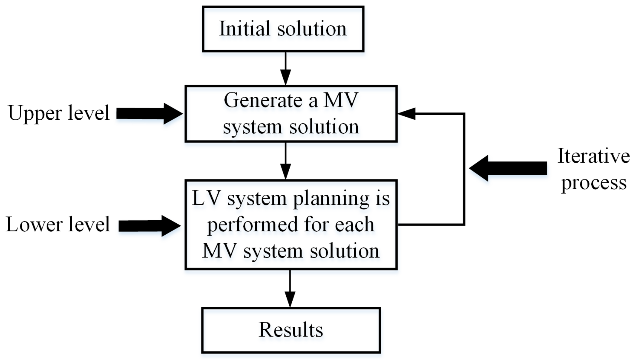
The central idea of this MV/LV planning decomposition search is to solve the LV systems for each solution of the MV system generated at the upper level; that is, for each MV solution generated at the upper level, a local search is performed to find the best LV system planning associated with this solution. This decomposition search process is represented by Figure 1. The LV system planning at the lower level is solved by the variable neighborhood descendent (VND) algorithm [38]. The search for the best MV/LV planning solution is accomplished through an iterative process between the MV and LV systems, considering the upper and lower level neighborhood sets.
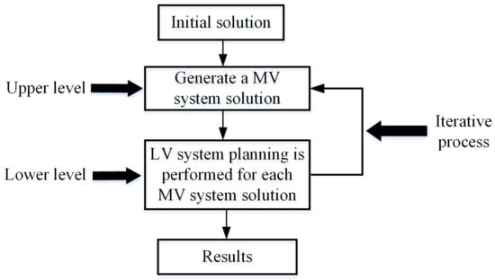
Figure 1.
Decomposition search.
The MV/LV system planning methodology using the decomposition search approach is presented in Algorithm 2. The algorithm starts, at Line 1, by building an initial MV/LV system solution using Algorithm 1. In Line 5, which represents the upper level, a solution for the MV system is generated using the neighborhood structure of the set k. For each MV solution generated, a local search in the lower level is performed using all LV neighborhood structures of set s (Lines 6–13). The stopping criterion (Line 20) consists of a predetermined number of iterations, after verifying that there was no improvement in the best solution found.
| Algorithm 2: MV/LV system planning methodology. |
|
5.4. Heuristic for Meshed Networks
Distribution systems are typically designed as a meshed network. Meshed systems allow for network reconfiguration in contingency cases through interconnection lines. Due to the complexity associated with the power system protection of meshed networks, distribution systems operate in a radial manner. The PAO and CAO used in this methodology always generate radial topologies. Thus, in this paper, an algorithm is proposed to install interconnection lines in the distribution system. Therefore, for each generated solution, Algorithm 3 is executed.
| Algorithm 3: Heuristic for meshed networks. |
|
The stopping criterion used in this algorithm consists of a predetermined number of iterations in which there is no improvement in the objective function.
5.5. Solution Evaluation
In this paper, original power flow equations are used to evaluate the planning solutions generated by the GVNS algorithm [39]. Although MV/LV solutions search are generated in a decomposed way, they are evaluated by a unique power flow, as the MV system influences the LV system and vice versa [39]. For each solution of the LV system, a heuristic finds the best tap position of each distribution transformer. The equality constraints presented in Equations (18)–(24) of the mathematical formulation are solved by a three-phase non-linear power flow [39]. The constraints presented in Equations (25)–(31), (37) and (38) are evaluated using penalty techniques [1,21]. The constraints in Equations (32)–(36) are guaranteed during the encoding phase.
6. Tests and Results
The algorithm was implemented in the C++ programming language, and tests were run on a server with an Intel (R) Xeon (R) processor, CPU E5-2630 v2, 3 GB of RAM, and 2.60 GHz.
6.1. System Data
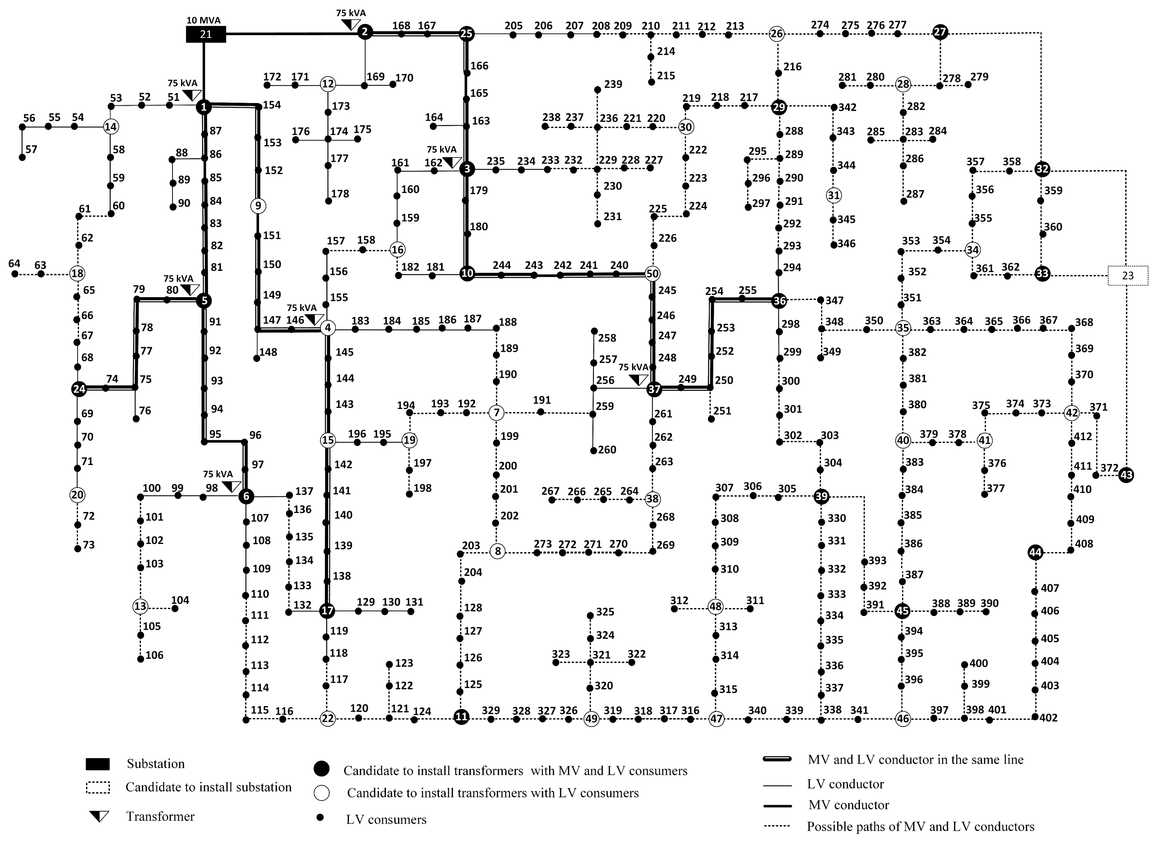
The proposed methodology was tested in an integrated MV/ LV distribution system composed of 50 MV nodes and 410 LV nodes. The system had one substation, seven distribution transformers, and some MV and LV lines in operation, providing energy to MV and LV consumers. A single-line diagram of the test system is shown in Figure 2. Electrical, financial, and physical data of the system, substations, distribution transformers, and MV and LV conductors, as well as the shared costs of conductors, poles, and support structures between the MV and LV networks, annual interest rate, power factor, the operating scenarios of our simulations, and the parameters used to calculate RPI can be found in [40]. The costs of poles, support structures, and cables, in addition to shared lines, were obtained using the table in [40]. This table presented the cost of installing or replacing a line with cables by cables , where m and p are MV cables and n and q are LV cables. The number of years of the planning horizon was equal to five, which is a typically period considered for expansion planning of distribution systems by DISCO.

Figure 2.
Test system.
In the test system used, it was considered that all nodes had the same demand and generation profile, as such profiles in distribution systems typically show this behavior. However, different demand and generation profiles for each bus could easily be incorporated into the problem, as these values are parameters for the model. In all study cases, system operation was modeled using scenarios that were generated by combining 8760 h of system demand, wind speed, and solar irradiation factors. Table 1 presents the demand , wind speed , and solar irradiation factors found by the scenario generation methodology presented in Section 2. Additionally, Table 1 presents the four operation blocks used to form the scenarios for the study cases analyzed in this paper. In addition, the time (in hours) belonging to each operation block is also presented. Operating times of each scenario were found by dividing the number of hours of each block by the number of scenarios used per block.

Table 1.
Operating scenarios.
In [40], the number of wind turbines and solar photovoltaic modules that were to be installed by independent owners in the planned distribution system was presented. The maximum active power generated by each wind turbine and photovoltaic module was 800 kW and 320 W, respectively. It was considered that all surplus energy generated by these RES was injected into the system. This energy surplus, which was obtained by a metering system, was considered as a credit to the consumer in other operating scenarios, where its demand was greater than its generation.
6.2. Numerical Results
Our simulations were divided into four case studies. Cases I and II showed the difference between MV/LV planning without considering the RPI and with the RPI, respectively. Case III showed the difference in the MV/LV planning considering RES. Case IV showed the trade-off between the costs of investment and operation versus the robustness of solutions in the MV/LV distribution system planning.
To prove the performance of the proposed planning methodology through the GVNS algorithm, several simulations were performed for the same case study. The algorithm found the same solution in 80% of tests, and in each case study, the variables of the problem were randomly initialized. Thus, the algorithm usually found the same solution through different paths of the search space. Another factor that demonstrated the efficiency and robustness of the algorithm, besides finding the same solution in most cases, was the small error difference between the best and the worst solutions found by the algorithm in the tests (i.e., less than 0.01%).
The results found by this algorithm were in accordance with the practical planning procedures of distribution systems. Furthermore, all solutions met the mathematical model constraints and the requirements of regulatory agencies for each operating scenario.
6.2.1. MV/LV Planning: Fixed Weight Factor
Case Studies I, II, and III considered a fixed weight factor in the objective function. Cases I and II performed MV/LV distribution system planning considering eight operational scenarios. These scenarios were generated by combining the eight demand factors and operation times of each block in Table 1. Case III considered 32 operational scenarios, which were obtained by combining the parameters of demand, wind speed, solar irradiation, and operation scenario time of each block in Table 1. The operating scenarios used in all case studies can be found in [40].
Case I: MV/LV distribution system planning was performed without considering the RPI; that is, with a weight factor in the objective function. This case did not consider RES.
Case II: MV/LV distribution system planning was performed considering the RPI; that is, with a weight factor in the objective function. This case did not consider RES.
Case III: MV/LV distribution system planning was performed considering RES. The RPI was not taken into account, with a weight factor in the objective function.
The costs of solutions obtained for Cases I, II, and III and the computational times (T; seconds) are presented in Table 2. Although the RPI was not taken into account in the objective function in Cases I and III, this index was still calculated.
Table 2.
Solutions (values: ).
Comparing Cases I and II, it can be observed that there was an increase in the costs of substations by 30%, distribution transformers by 97.30%, and conductors, poles, and structures by 17.40%, when the RPI was taken into account in the mathematical model. Case II had a significantly higher robustness index, compared to Case I.
To show how the RPI influenced MV/LV planning, we compared the power of substations and distribution transformers, current in cables, and voltage at consumption points, in relation to their maximum limits, in Cases I and II. This analysis was performed by considering the peak load scenario.
In Cases I and II, one substation was installed at Node 21 and another at Node 23. In Case I, the installed power in substations at nodes 21 and 23 were 17.5 MVA and 12.5 MVA, respectively; in Case II, they were 20 MVA and 17.5 MVA, respectively. In Case I, the peak load scenarios in these substations were 17.22 MVA and 12.47 MVA, respectively; in Case II, they were 17.02 MVA and 12.57 MVA, respectively. Therefore, in Cases I and II, there was 1.04% and 26.72% available power in these substations, respectively, which could meet higher demand. This demonstrated that the RPI (which was considered in Case II) reduced the risk of overpower in these substations.
Regarding distribution transformers, it was observed that, in Case I, there were 15 distribution transformers that were very close to their maximum power limits, with a maximum capacity of 5% available to meet higher demand. In Case II, there was no distribution transformer operating under these conditions. The distribution transformer closest to its limit had 37.92% of power available to meet other loads. In Case II, in addition to the higher cost of transformers, we noted that 47 transformers were installed; whereas in Case I, only 34 transformers were installed.
Regarding the current levels in the MV and LV systems, the same behavior associated with distribution transformers was verified. In Case I, there were six and 10 conductors in the MV and LV systems, respectively, with a maximum of 5% of current capacity available. In Case II, there were no conductors under these conditions in either the MV or LV system. In the MV and LV systems, the conductors closest to their limits had 21.95% and 9.27% of their current capacity available, respectively.
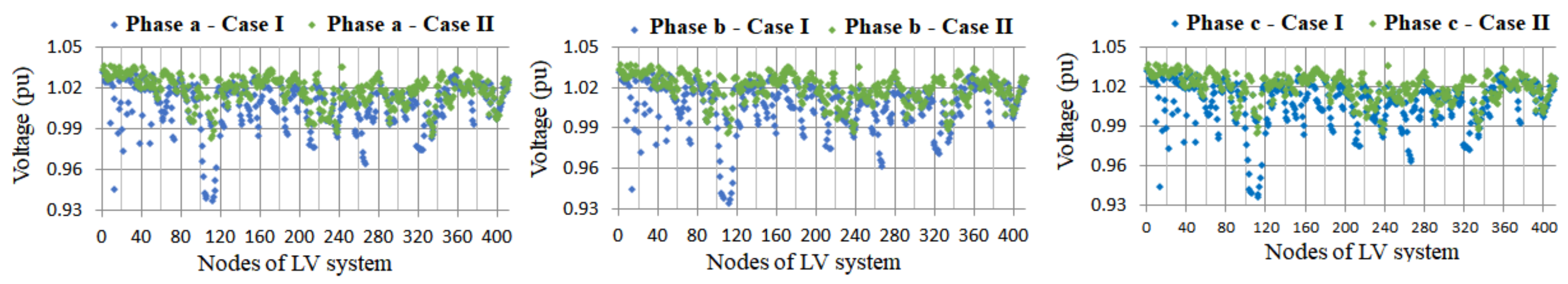
We can observe that the voltage regulation was also better in Case II. In Case I, there were 23 consumption points with voltage deviation greater than 5% of their nominal power; meanwhile, in Case II, there were no consumption points operating under these conditions. Figure 3 presents the voltage levels of the LV system, which was the network with the largest voltage drop. The results showed that the RPI improved the voltage stability in Case II.

Figure 3.
Voltage in the LV system: Cases I and II.
The results presented in Case III showed that the higher the power injected by RES, the lower the costs related to investments and operation. In Case III, there was a reduction of 11.23% in distribution transformer costs; 11.70% in cable, pole, and structural costs; and 28.44% in power losses costs, when compared to Case I. Furthermore, the results showed that the largest number of installed distribution transformers occurred in Case II (with 47 transformers); while the smallest number of transformers occurred in Case III (with 27 transformers). These results showed that the RPI (considered in Case II) increased the number of transformers, and RES (considered in Case III) decreased this number. It can also be noted that Case III had the lowest robustness index, while Case II had the highest one.
6.2.2. MV/LV Planning: Variable Weight Factor
A multiobjective approach was performed in Case IV, with the weight factor, , in the objective function varying from to , in increments of .
Case IV: MV/LV distribution system planning was performed considering RES and RPI. Several cases were performed with 32 operating scenarios, searching for a trade-off between the costs of investment and operation versus the robustness of solutions. Operating scenarios were obtained from load demand, solar irradiation, and wind speed factors combined with the operation times of each block.
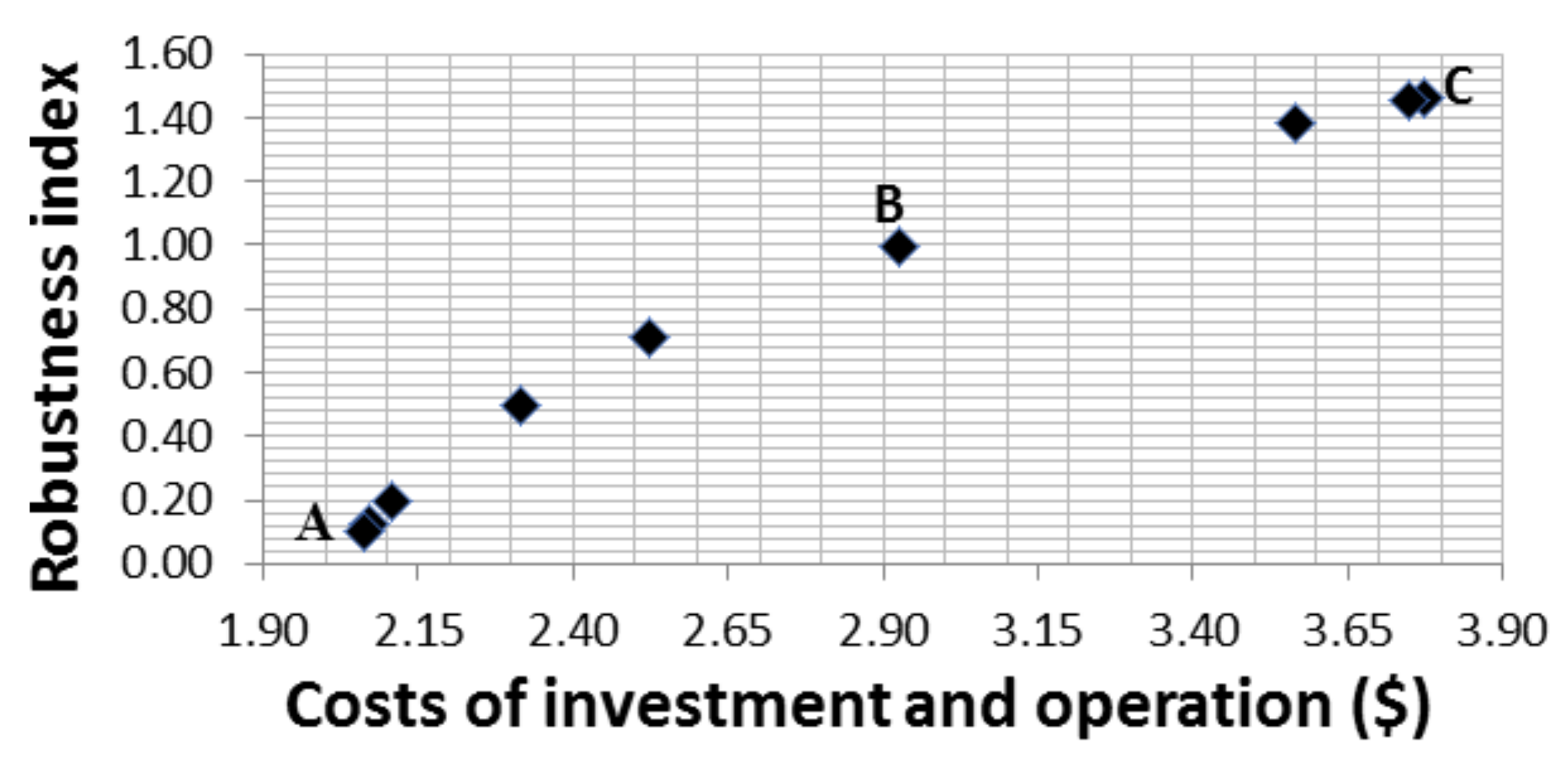
Figure 4 presents the trade-off between investment and operation costs versus the robustness in the proposed MV/LV planning solutions.

Figure 4.
Frontier obtained: Case IV (values: ).
The results obtained showed that, for example, for Solution A (with ) in Figure 4, the investment and operation costs were lower compared with the other solutions; the robustness was lower as well. On the other hand, in Solution C (with ), the investment and operating costs in the distribution system were higher compared with the other cases, and the robustness index was also greater. Solution B provided an intermediate solution between the costs of investment and operation and robustness. Thus, in Solution A, there was a higher risk that the physical and operational characteristics of the equipment were exceeded and an overpower, overvoltage, or overcurrent occurred. Therefore, with these results, the DISCO could choose the most viable planning solution, considering their physical, economic, environmental, and robustness criteria. For a more detailed analysis, the costs from to , including the costs of Solutions A, B, and C (with , , and , respectively), are presented in Table 3.
Table 3.
Solutions (values: ).
The results in Table 3 show an increase of the costs of substations by 80%, distribution transformers by 191.93%, and for conductors, poles, and structures by 88.05%, when comparing Solutions A and C. On the other hand, Solution C was much more robust and resilient than Solution A. In Solutions A and C, one substation was installed at Node 21 and another at Node 23. In Solution A, the installed power capacities in these substations were 17.5 MVA and 12.5 MVA, respectively; for Solution C, these were both 25 MVA. In Solution A, the peak load scenarios in these substations were 16.51 MVA and 12.04 MVA, respectively; for Solution C, these were 17.47 MVA and 10.95 MVA, respectively. Therefore, in Solutions A and C, there was 5.08% and 75.92% available power at the substations, respectively, to meet higher demand. Regarding the distribution transformers, in Solution A, there were three distribution transformers with a maximum 5% of available power capacity. In Solution C, there was no distribution transformer under these conditions. The results presented in Solution C thus reduced the risk of overpower in substations and distribution transformers. Regarding current levels, in Solution A, there were six and 16 cables in the MV and LV systems, respectively, with a maximum of 5% of available current capacity. In Solution C, there were no conductors in the MV and LV systems under these conditions, reducing the risk of overcurrent. Regarding the voltage levels, in Solution A, there were 10 consumption points with voltage deviations greater than 5%; in Solution C, there were no consumption points under these conditions, reducing the risk of overvoltage and undervoltage in the distribution system.
The results showed that the weight factor value, besides influencing the investment and operation costs, also influenced the number of distribution transformers installed. For the case with , forty-seven transformers were installed; whereas, with , thirty-three transformers were installed.
For a better understanding of the MV/LV integrated planning performed in this work, we present the single-line diagrams for Solution B in Figure 5 and for solutions A and C in the Appendix A (Figure A1 and Figure A2). Through these figures, it is possible to visualize all the routes of the MV, LV, and MV/LV shared lines installed, interconnection lines, as well as the positions and capacities of distribution transformers installed, substation capacities, and the positions of wind and solar generators considered in the MV/LV planning.
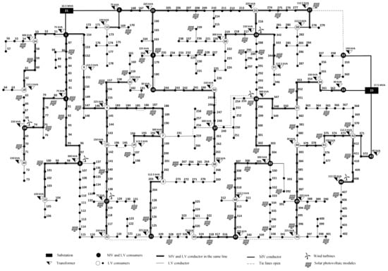
Figure 5.
Solution B.
From the case studies analyzed, it could be verified that the most drastic cost reduction occurred in MV, where the highest power injection was concentrated by the wind generators when compared to LV. In addition, it was found that the lowest investment costs occurred when the RES were closer to the demand points of the system. RES also allowed us to reduce the values of currents and to increase the levels of the voltage magnitudes, improving the standards of operation of the planned system.
The routes of MV feeders and LV circuits for the distribution system were different for most case studies analyzed. The quantity, position, and capacity of the distribution transformers, in addition to the types of MV and LV conductors installed, were also different. This showed that RES and the RPI influenced MV/LV solution planning.
7. Conclusions
The proposed solution technique using an MV/LV planning decomposition search approach with the GVNS was shown to be robust and efficient. The results obtained through the proposed methodology showed that it was possible to find robust and resilient solutions, besides reducing the investment and operation costs of a distribution system, with the integration of RES.
The RPI proposed in this paper was able to find more conservative and resilient MV/LV planning solutions, with lower risks of overpower, overvoltage, and overcurrent occurrences. On the other hand, it could be observed that solutions with lower robustness were economically more attractive, whereas solutions with greater robustness were more expensive, but more reliable and resilient.
RES reduced the infrastructural costs of the network, such as distribution transformers, conductors, poles, isolated support structures, and shared MV/LV lines, as well as the costs of system losses. RES also allowed for increasing the voltage levels at the load points, thus improving the efficiency and quality standards of the system. Regarding the environmental aspects, RES also allowed us to reduce the amount of greenhouse gas emissions.
Therefore, the proposed methodology appeals to engineers responsible for distribution system planning, providing a more realistic decision-making framework that takes into account how to reduce the costs of investment and operation while preserving the necessary robustness inherent in MV/LV planning solutions. In this way, DISCOs can choose the level of robustness of the distribution system, taking into account their financial constraints.
Author Contributions
Conceptualization, D.R., B.R.P.J., J.C., and J.R.S.M.; methodology, D.R., B.R.P.J., J.C., and J.R.S.M.; software, D.R.; validation, D.R; formal analysis, D.R., B.R.P.J., J.C., and J.R.S.M.; investigation, D.R.; resources, D.R., B.R.P.J., J.C., and J.R.S.M.; data curation, D.R.; writing, original draft preparation, D.R; writing, review and editing, B.R.P.J., J.C., and J.R.S.M.; visualization, D.R.; supervision, J.C. and J.R.S.M.; project administration, D.R. and J.R.S.M.; funding acquisition, D.R. and J.R.S.M. All authors read and agreed to the published version of the manuscript.
Funding
This work is supported by: São Paulo Research Foundation (FAPESP), under the Grants 2017/13599-9, 2018/21610-5, and 2015/21972-6; “Coordenação de Aperfeiçoamento de Pessoal de Nível Superior—Brazil (CAPES)—Finance Code 001”; National Council for Scientific and Technological Development (CNPq), under Grant 305318/2016-0; the Ministry of Science, Innovation and Universities of Spain, under Projects RTI2018-096108-A-I00 and RTI2018-098703-B-I00 (MCIU/AEI/FEDER, UE); Universidad de Castilla-La Mancha, under Grant 2019-GRIN-26950.
Conflicts of Interest
The authors declare no conflict of interest.
Nomenclature
| Sets | |
| , | set of conductor types of the MV and LV systems, respectively |
| set of renewable generation units | |
| , | set of existing and future lines of MV and LV systems, respectively |
| set of existing and future lines of the MV/LV system | |
| , | set of nodes of MV and LV systems, respectively |
| set of nodes of existing or proposed substations and transformers, respectively | |
| set of operating scenarios | |
| set of system phases a, b, and c | |
| set of substation and distribution transformer types, respectively | |
| set of transformer tap positions | |
| Parameters | |
| a | tap variation of distribution transformer |
| cost to change cables , where m is an MV cable and n is an LV cable, for cables , where p is an MV cable and q is an LV cable, in branch ($) | |
| cost of losses in scenario w, in year t ($/MWh) | |
| cost of substation and transformer k installed at bus i, respectively | |
| maximum financial resource for planning | |
| maximum current through line (A) | |
| annual interest rate (%) | |
| losses of iron and copper in substation k, respectively (MW) | |
| losses of iron and copper in transformer k, respectively (MW) | |
| number of years of the planning horizon | |
| active and reactive power demand at bus i in scenario w, in year t, respectively (MW, MVAr) | |
| maximum active power generation from DG at bus i (MW) | |
| maximum loading of substation and transformer k installed at bus i, respectively (MVA) | |
| duration of each operation block b in year t (h) | |
| duration of each operation scenario w in year t (h) | |
| power factor | |
| , | minimum and maximum voltage limits at bus i, respectively |
| nominal voltage at bus i | |
| robust index weight associated with the DG in operating scenario w in year t | |
| robust index weight associated with the voltages of MV and LV systems in operating scenario w, in year t, respectively | |
| robust index weight associated with the current through cables installed in MV and LV systems in operating scenario w, in year t, respectively | |
| robust index weight associated with substations and distribution transformers in operating scenario w, in year t, respectively | |
| impedance of distribution transformer k installed at bus i (%) | |
| discretisation interval of transformer tap | |
| weight factor associated with the objective function | |
| Variables | |
| , | binary decision variable that defines the operation of MV and LV cables of type k in branch , respectively |
| financial resource for planning | |
| current in phase f, through line in scenario w, in year t (A) | |
| , | currents at the MV and LV levels, in transformer i in scenario w, in year t, respectively (A) |
| magnetizing current of the MV/LV distribution transformer at node i in scenario w, in year t (A) | |
| power losses in the cables of MV and LV systems in year t, respectively (MW) | |
| power losses at substations and transformers in year t, respectively (MW) | |
| , | active and reactive power injections at bus i in scenario w, in year t, respectively (MW, MVAr) |
| , | active and reactive power generated at bus i in scenario w, in year t, respectively (MW, MVAr) |
| power demanded by substation i in scenario w, in year t (MVA) | |
| power demanded by transformer i in scenario w, in year t (MVA) | |
| , | power consumption in substation and transformer i in scenario w, in year t, respectively (MVA) |
| , | binary decision variable for the installation of substations and distribution transformer of type k at bus i, respectively |
| , | power supplied by substation and transformer i in operation scenario w, in year t, respectively (MVA) |
| V | voltage in the node |
| , | voltage magnitude in phase f, at nodes i and j in scenario w, in year t, respectively (V) |
| , | input voltage magnitude of the MV system and output of the LV system in transformer i in scenario w, in year t, respectively (V) |
| nodal phase angle |
Appendix A

Figure A1.
Solution A.
Figure A1.
Solution A.
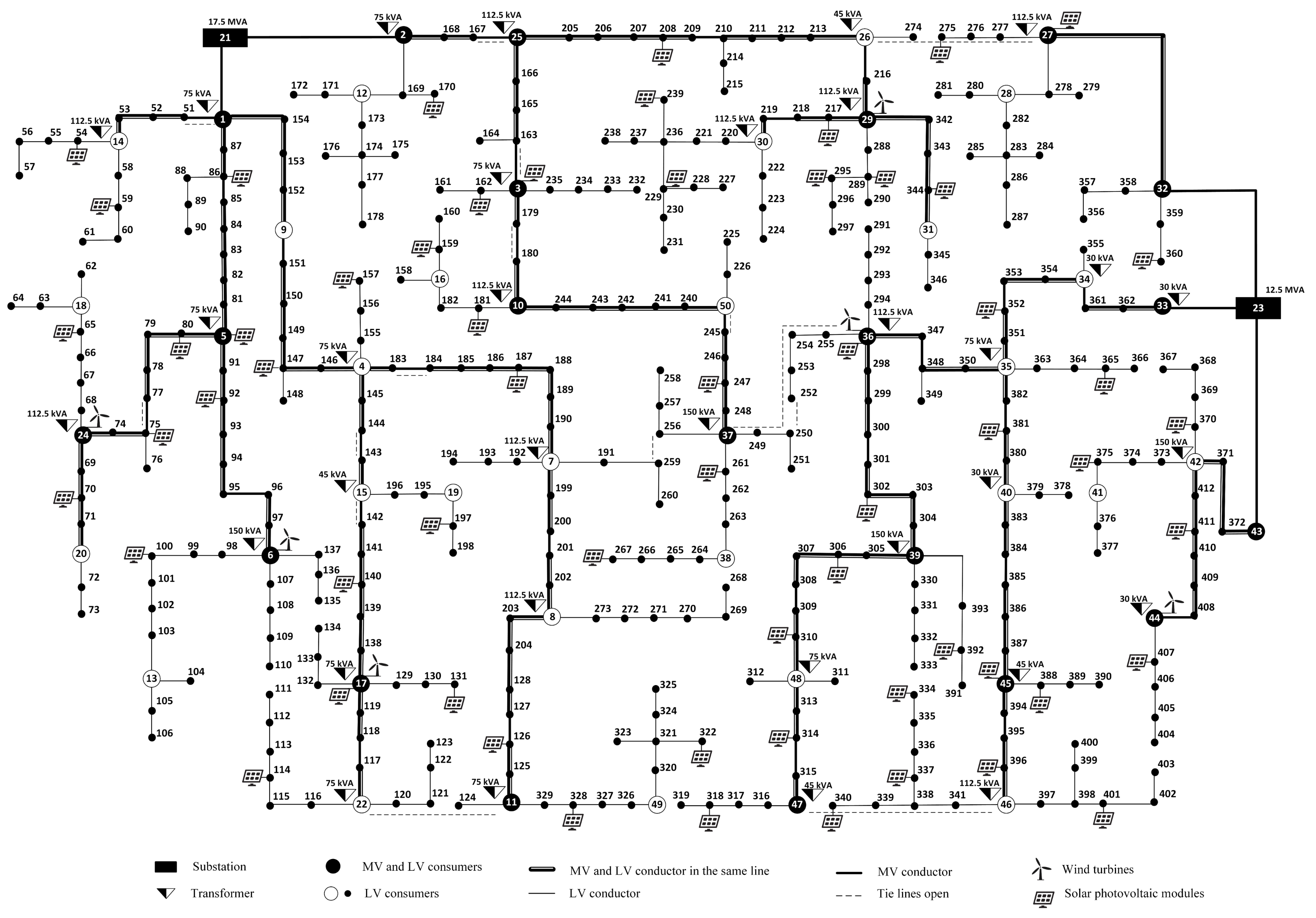

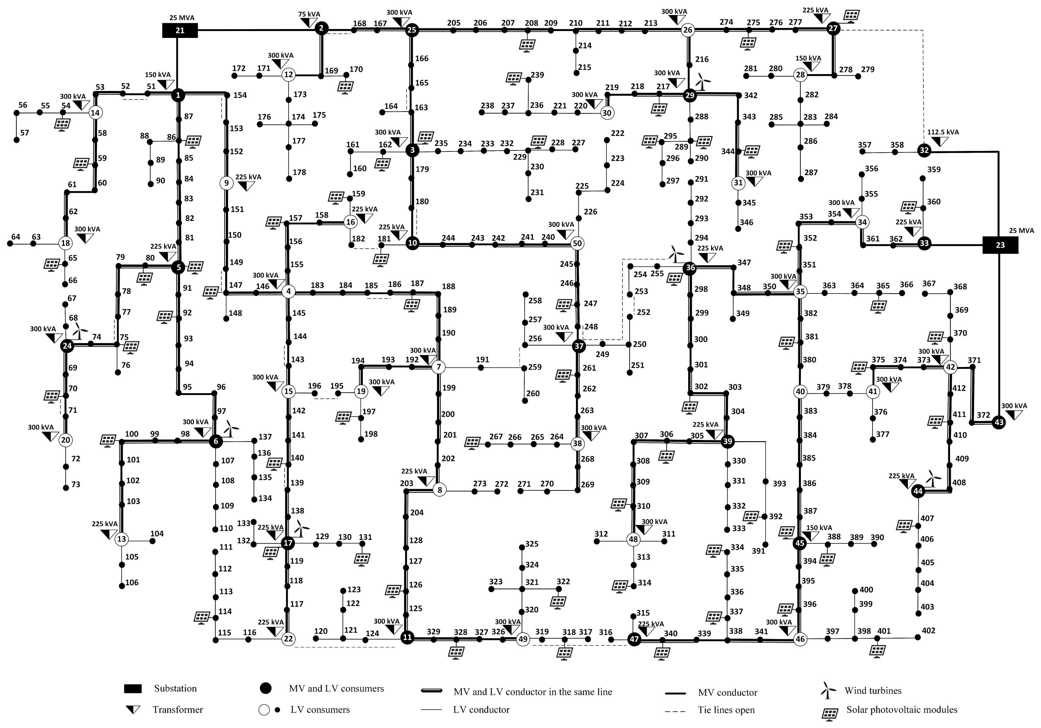
Figure A2.
Solution C.
Figure A2.
Solution C.
References
- Viral, R.; Khatod, D.K. Optimal planning of distributed generation systems in distribution system: A review. Renew. Sustain. Energy Rev. 2012, 16, 5146–5165. [Google Scholar] [CrossRef]
- El-Khattam, W.; Bhattacharya, K.; Hegazy, Y.; Salama, M.M.A. Optimal investment planning for distributed generation in a competitive electricity market. IEEE Trans. Power Syst. 2004, 19, 1674–1684. [Google Scholar] [CrossRef]
- Singh, R.K.; Goswami, S.K. Optimum allocation of distributed generations based on nodal pricing for profit, loss reduction, and voltage improvement including voltage rise issue. Int. J. Electr. Power Energy Syst. 2010, 32, 637–644. [Google Scholar] [CrossRef]
- Muñoz-Delgado, G.; Contreras, J.; Arroyo, J.M. Multistage Generation and Network Expansion Planning in Distribution Systems Considering Uncertainty and Reliability. IEEE Trans. Power Syst. 2016, 31, 3715–3728. [Google Scholar] [CrossRef]
- Montoya-Bueno, S.; Muñoz, J.I.; Contreras, J. A Stochastic Investment Model for Renewable Generation in Distribution Systems. IEEE Trans. Sustain. Energy 2015, 6, 1466–1474. [Google Scholar] [CrossRef]
- Acharya, N.; Mahat, P.; Mithulananthan, N. An analytical approach for DG allocation in primary distribution network. Int. J. Electr. Power Energy Syst. 2006, 28, 669–678. [Google Scholar] [CrossRef]
- Gözel, T.; Hocaoglu, M.H. An analytical method for the sizing and siting of distributed generators in radial systems. Electr. Power Syst. Res. 2009, 79, 912–918. [Google Scholar] [CrossRef]
- Hung, D.Q.; Mithulananthan, N.; Bansal, R.C. Analytical Expressions for DG Allocation in Primary Distribution Networks. IEEE Trans. Energy Convers. 2010, 25, 814–820. [Google Scholar] [CrossRef]
- Atwa, Y.M.; El-Saadany, E.F.; Salama, M.M.A.; Seethapathy, R. Optimal Renewable Resources Mix for Distribution System Energy Loss Minimization. IEEE Trans. Power Syst. 2010, 25, 360–370. [Google Scholar] [CrossRef]
- Ghosh, S.; Ghoshal, S.; Ghosh, S. Optimal sizing and placement of distributed generation in a network system. Int. J. Electr. Power Energy Syst. 2010, 32, 849–856. [Google Scholar] [CrossRef]
- El-Zonkoly, A.M. Optimal placement of multi-distributed generation units including different load models using particle swarm optimisation. IET Gener. Transm. Distrib. 2011, 5, 760–771. [Google Scholar] [CrossRef]
- Borges, C.L.T.; Falcão, D.M. Optimal distributed generation allocation for reliability, losses, and voltage improvement. Int. J. Electr. Power Energy Syst. 2006, 28, 413–420. [Google Scholar] [CrossRef]
- Celli, G.; Ghiani, E.; Mocci, S.; Pilo, F. A multiobjective evolutionary algorithm for the sizing and siting of distributed generation. IEEE Trans. Power Syst. 2005, 20, 750–757. [Google Scholar] [CrossRef]
- Hedayati, H.; Nabaviniaki, S.A.; Akbarimajd, A. A Method for Placement of DG Units in Distribution Networks. IEEE Trans. Power Deliv. 2008, 23, 1620–1628. [Google Scholar] [CrossRef]
- Rau, N.S.; Wan, Y.-H. Optimum location of resources in distributed planning. IEEE Trans. Power Syst. 1994, 9, 2014–2020. [Google Scholar] [CrossRef]
- El-Khattam, W.; Hegazy, Y.G.; Salama, M.M.A. An integrated distributed generation optimization model for distribution system planning. IEEE Trans. Power Syst. 2005, 20, 1158–1165. [Google Scholar] [CrossRef]
- Zheng, Y.; Dong, Z.Y.; Meng, K.; Yang, H.; Lai, M.; Wong, K.P. Multi-objective distributed wind generation planning in an unbalanced distribution system. CSEE J. Power Energy Syst. 2017, 3, 186–195. [Google Scholar] [CrossRef]
- Naderi, E.; Seifi, H.; Sepasian, M.S. A Dynamic Approach for Distribution System Planning Considering Distributed Generation. IEEE Trans. Power Deliv. 2012, 27, 1313–1322. [Google Scholar] [CrossRef]
- Khalesi, N.; Rezaei, N.; Haghifam, M. DG allocation with application of dynamic programming for loss reduction and reliability improvement. Int. J. Electr. Power Energy Syst. 2011, 33, 288–295. [Google Scholar] [CrossRef]
- Banerjee, B.; Islam, S.M. Reliability based optimum location of distributed generation. Int. J. Electr. Power Energy Syst. 2011, 33, 1470–1478. [Google Scholar] [CrossRef]
- Falaghi, H.; Singh, C.; Haghifam, M.; Ramezani, M. DG integrated multistage distribution system expansion planning. Int. J. Electr. Power Energy Syst. 2011, 33, 1489–1497. [Google Scholar] [CrossRef]
- Singh, D.; Singh, D.; Verma, K.S. Multiobjective Optimization for DG Planning with Load Models. IEEE Trans. Power Syst. 2009, 24, 427–436. [Google Scholar] [CrossRef]
- Placement of distributed generators and reclosers for distribution network security and reliability. Int. J. Electr. Power Energy Syst. 2005, 27, 398–408. [CrossRef]
- Keane, A.; O’Malley, M. Optimal allocation of embedded generation on distribution networks. IEEE Trans. Power Syst. 2005, 20, 1640–1646. [Google Scholar] [CrossRef]
- Alkaabi, S.S.; Zeineldin, H.H.; Khadkikar, V. Adaptive planning approach for customer DG installations in smart distribution networks. IET Renew. Power Gener. 2018, 12, 81–89. [Google Scholar] [CrossRef]
- Billinton, R.; Karki, R. Maintaining supply reliability of small isolated power systems using renewable energy. IEE Proc. Gener. Transm. Distrib. 2001, 148, 530–534. [Google Scholar] [CrossRef]
- Rupolo, D.; Pereira Junior, B.R.; Contreras, J.; Mantovani, J.R.S. Medium- and low-voltage planning of radial electric power distribution systems considering reliability. IET Gener. Transm. Distrib. 2017, 11, 2212–2221. [Google Scholar] [CrossRef]
- Yosef, M.; Sayed, M.M.; Youssef, H.K.M. Allocation and sizing of distribution transformers and feeders for optimal planning of MV/LV distribution networks using optimal integrated biogeography based optimization method. Electr. Power Syst. Res. 2015, 128, 100–112. [Google Scholar] [CrossRef]
- Paiva, P.C.; Khodr, H.M.; Dominguez-Navarro, J.A.; Yusta, J.M.; Urdaneta, A.J. Integral planning of primary-secondary distribution systems using mixed integer linear programming. IEEE Trans. Power Syst. 2005, 20, 1134–1143. [Google Scholar] [CrossRef]
- Fletcher, R.H.; Strunz, K. Optimal Distribution System Horizon Planning; Part I: Formulation. IEEE Trans. Power Syst. 2007, 22, 791–799. [Google Scholar] [CrossRef]
- Fletcher, R.H.; Strunz, K. Optimal Distribution System Horizon Planning; Part II: Application. IEEE Trans. Power Syst. 2007, 22, 862–870. [Google Scholar] [CrossRef]
- Amjady, N.; Attarha, A.; Dehghan, S.; Conejo, A.J. Adaptive Robust Expansion Planning for a Distribution Network with DERs. IEEE Trans. Power Syst. 2018, 33, 1698–1715. [Google Scholar] [CrossRef]
- Zhang, C.; Xu, Y.; Dong, Z.Y. Probability-Weighted Robust Optimization for Distributed Generation Planning in Microgrids. IEEE Trans. Power Syst. 2018, 33, 7042–7051. [Google Scholar] [CrossRef]
- Zare, A.; Chung, C.Y.; Zhan, J.; Faried, S.O. A Distributionally Robust Chance-Constrained MILP Model for Multistage Distribution System Planning with Uncertain Renewables and Loads. IEEE Trans. Power Syst. 2018, 33, 5248–5262. [Google Scholar] [CrossRef]
- Gazijahani, F.S.; Salehi, J. Robust Design of Microgrids with Reconfigurable Topology Under Severe Uncertainty. IEEE Trans. Sustain. Energy 2018, 9, 559–569. [Google Scholar] [CrossRef]
- Taylor, J.A. Convex Optimization of Power Systems; Cambridge University Press: Cambridge, UK, 2015; Volume 1. [Google Scholar]
- Delbem, A.C.B.; de Carvalho, A.; Policastro, C.A.; Pinto, A.K.O.; Honda, K.; Garcia, A.C. Node-Depth Encoding for Evolutionary Algorithms Applied to Network Design. In Genetic and Evolutionary Computation– GECCO 2004; Deb, K., Ed.; Springer: Berlin/Heidelberg, Germany, 2004; pp. 678–687. [Google Scholar]
- Mladenovic, N.; Hansen, P. Variable Neighborhood Search; Kluwer Academic Publishers: Berlin, Germany, 2003; Volume 1, pp. 145–184. [Google Scholar]
- Cheng, C.S.; Shirmohammadi, D. A three-phase power flow method for real-time distribution system analysis. IEEE Trans. Power Syst. 1995, 10, 671–679. [Google Scholar] [CrossRef]
- MV/LV Test System. Available online: https://drive.google.com/open?id=1Tba34jHNUk1S7MY4EFaHBsM1sli9lJ9j (accessed on 16 October 2019).

© 2020 by the authors. Licensee MDPI, Basel, Switzerland. This article is an open access article distributed under the terms and conditions of the Creative Commons Attribution (CC BY) license (http://creativecommons.org/licenses/by/4.0/).