The Response of US Macroeconomic Aggregates to Price Shocks in Crude Oil vs. Natural Gas

Abstract

Price fluctuations in crude oil and natural gas, as important sources of energy, have a remarkable influence on our economies and daily lives. Therefore, it is extremely important to react appropriately and to formulate appropriate policies or strategies to reduce the expected negative effects of fluctuations. However, as Kilian suggested, not all oil price shocks are similar; price increases can have diverse impacts on the real price of oil, depending on the underlying determinants of the price fluctuation. Therefore, economists, policymakers, and investors need to decompose real price shocks and evaluate the responses of macroeconomic aggregates to different types of shocks. In this study, we investigate and compare the different effects crude oil and natural gas price shocks have on US real GDP and CPI levels, utilizing a two-stage method based on a structural vector autoregression (SVAR) model proposed by Kilian. We found that a crude oil specific demand shock made larger contributions to the real price of oil than a natural gas specific demand shock did to the real price of gas, and that specific demand shocks in crude oil and natural gas markets had different effects on US CPI inflation and had similar effects on the real US GDP level.

1. Introduction

Researchers have studied crude oil for many years because it is of major interest as a significant but limited resource. In addition, the crude oil index plays an important role among economists, policymakers, and investors, because fluctuations in either its price or its production have a remarkable impact on the world economy and stock markets. On the contrary, as a relatively environmentally friendly resource and a key fuel for the electrical power and industry sectors, natural gas has attracted increasing attention. Evidence for this increasing attraction comes from the fact that the consumption of natural gas has risen to a share of 23% of total energy resources, and is the fastest-growing fossil fuel among energy resources [1]. Another fact is that the demand for natural gas increased by 4.6% in 2018, accounting for almost half of all energy resource demand growth [2]. Thus, it is not difficult to conclude that fluctuations in the prices of crude oil and natural gas greatly influence economic activity and daily life.

Researches had shown that there is a correlation between US economic growth and exogenous oil shocks. For instance, Hamilton [3,4] and Hooker [5] proposed that after oil price increases, there were recessions in the US economy. However, as proposed by Kilian [6], depending on the underlying causes, such as supply shocks, aggregate demand, or precautionary demand, price fluctuations have varying dynamic effects on real prices, and hence on the economy. Other studies have agreed; for instance, Kling [7] reported that the association is obvious between crude oil price increases and declines in the stock market. However, Kilian and Park [8] reported that US real stock returns reacted differently to oil price shocks, depending on the origins driving the oil price shocks. Other research has also analyzed the macroeconomic effects of oil market fluctuations. Oladosu et al. [9] adopted a quantitative meta-regression model to simulate the oil price elasticity of GDP in US and their results revealed that the estimated US GDP elasticity was negative, and particularly smaller than about 10 years ago. Jan van de Ven and Fouquet [10] identified the impact of energy shocks on economic activity using data from the United Kingdom for 310 years and their study indicated that the influences of supply shocks declined due to the partial shift from coal to crude oil, and that it is possible to reduce vulnerability and increase resilience by substituting renewable energy sources for traditional energy sources. Ju et al. [11] used data from 1980 to 2014 to investigate the macroeconomic performance of oil price shocks by adopting three methods, namely, empirical covariance, robust covariance, and support vector machine methods, and the results implied that the outlier performances of GDP, CPI, and the unemployment rate are consistent with the oil price shock process. Correspondingly, some literature investigated the relationship between natural gas price shocks and macroeconomic aggregates. Nick and Thoenes [12] extended the structural vector autoregression (SVAR) model and analyzed the effects of different fundamental influences on the price of natural gas in the German market. Their results revealed that in the short-term, the price of natural gas tends to be affected by some factors, such as temperature, inventory, and supply insufficiencies, and, by contrast, in the long-term the price tends to be influenced by the overall economic climate and the substitutional relationship between crude oil and coal. Zhang et al. [13] used a computable general equilibrium model to investigate the macroeconomic effects of natural gas prices in China and their results showed that when natural gas prices increase, the CPI would increase and GDP would decrease. In addition, research has also emphasized the transmission effect of oil demand and supply shocks on the natural gas market. For example, Jadidzadeh and Serletis [14] analyzed the effects of supply-demand shocks stemming from the global oil market on the real price of natural gas and found that oil supply-demand shocks accounted for approximately 45% of the fluctuation in the price of natural gas.

This study’s first objective is to decompose shocks to the real price of crude oil and natural gas into three components: (1) oil/gas supply shocks, (2) global aggregate demand shocks, and (3) specific or precautionary demand shocks. Its second objective is to evaluate important differences in how US macroeconomic aggregates, such as CPI and real GDP growth, react to various oil shocks underlying the real price of crude oil and natural gas. The third objective of this study is to compare its results with Kilian’s results regarding crude oil in 2009, in order to determine whether conditions have changed since 2007. Our data cover the period from 1973:1 to 2019:6, whereas Kilian [6] only had data up to 2007:12. Its fourth objective is to compare the impacts on crude oil and natural gas of different types of shocks to US macroeconomic aggregates. We expect this study to have implications for market operators and investors.

Because one of the objectives of our study is to compare our results with Kilian’s work, and because we used the same approach as Kilian [6], there is a necessity to demonstrate the similarities and discrepancies between the two works. We used the same methodology and variables as in Kilian’s work. However, because the importance and the potentiality of natural gas has gradually increased, we added natural gas to our study to check the effects of each structural shock on the real price of oil and gas and compare their effects on the US macroeconomic aggregates; in contrast, Kilian’s work focused on the crude oil market. Another difference is that our sample period of crude oil is longer than Kilian’s to verify if there are any changes after 2007.

Our findings in this study are threefold. First, by constructing an SVAR model to quantify the responses to one-standard-deviation structural shocks, we found that there were differences between the effects on crude oil and natural gas in the response patterns of real economic activity due to precautionary demand shocks. Second, by decomposing historic real prices to check the cumulative contribution from each demand and supply shock to the real price, we found that the cumulative effect of precautionary demand shocks was varying in degree between crude oil and natural gas; specifically, the cumulative contribution of an oil-specific demand shock to the real oil prices is larger than the cumulative contribution of a gas-specific demand shock to the real gas prices. Third, by utilizing the regression model to investigate how oil and gas demand and supply shocks that underlie the real price of oil and gas influence US macroeconomic aggregates, we found that precautionary demand shocks on crude oil and natural gas have different effects on CPI inflation and had similar effects on real GDP growth. Both oil- and gas-specific demand shocks led to a small, but statistically insignificant, reduction of the US GDP level. Oil-specific demand shocks tended to cause a large and statistically significant increase in CPI inflation; by contrast, gas market-specific demand shocks led to a small and statistically insignificant increase in the US CPI level. This result implied policymakers should react differently to gas-specific demand shocks and oil-specific demand shocks.

The remainder of this paper is organized as follows. Section 2 provides a detailed description of the data and introduces the econometric model, a two-stage method based on the SVAR model proposed by Kilian [6]. Section 3 identifies the structural shocks that drive the real price of crude oil and natural gas. We quantify the historical evolution of these shocks and the response to these shocks from production, real activity, and the real price of crude oil and natural gas. We decompose the real price of crude oil and natural gas over time to assess the respective cumulative contribution of each shock to real prices. Finally, we analyze the effects of those shocks on US macroeconomic aggregates. Section 4 concludes the study.

2. Materials and Methods

2.1. Data

Table 1. Data descriptions and sources.

Variable	Sample Period	Frequency	Description	Data Source
$\Delta opro{d}_t$	1973:1–2019:6	monthly	Percentage change in global crude oil production	IEA 2
$l\_re{a}_t$	1973:1–2019:6	monthly	Logarithmic real economic activity index (Kilian index)	Lutz Kilian website [15]
$l\_rp{o}_t$	1973:1–2019:6	monthly	Log real price of crude oil 1	Federal Reserve Bank
$\Delta gpro{d}_t$	1994:1–2019:6	monthly	Percentage change in global natural gas production	IEA 2
$l\_rp{g}_t$	1994:1–2019:6	monthly	Log real price of natural gas 1	Federal Reserve Bank
gdp_gr	1973:1–2019:6	quarterly	Real US GDP growth	OECD
cpi	1973:1–2019:6	quarterly	US CPI	OECD

¹ Real price means price which is deflated by US CPI. ² Data from the International Energy Agency.

describes the datasets we utilized and their sources. These datasets included crude oil production, gas production, a real economic activity index (the Kilian index available on his website), crude oil prices, natural gas prices, and US real GDP, deflated using US CPI (Kilian [6]).

We collected data from Bloomberg, Thomson Reuters, and OECD Stat. These datasets include the crude oil spot price (West Texas Intermediate, WTI) and the natural gas spot price (Henry Hub). $l\_rp{o}_t$ defers to the real price of crude oil expressed in log terms. $l\_rp{g}_t$ defers to the real price of natural gas expressed in log terms. Regarding the dataset of the Kilian index, we collected the data from the Lutz Kilian website. From Kilian (2009), the Kilian index is a detrended real freight rate index constructed as a measure of monthly global real economic activity, which could imply the variation of worldwide real economic activity and capture the shifts in the demand for industrial commodities throughout international markets [6,15] (see Appendix A for details). In this study, $l\_re{a}_t$ defers to the Kilian index; because the minimum of the Kilian index is −161.643, we added 196 to every data point and expressed the series in log terms. We collected production data for oil and gas from the International Energy Agency (IEA), and calculated the change rate of oil/gas production in percentage terms to reflect the percentage change of worldwide oil/gas production. $\Delta opro{d}_t$ refers to the percentage change in global crude oil production, and $\Delta gpro{d}_t$ refers to the percentage change in global natural gas production. US real GDP growth and US CPI data was collected from the Organization for Economic Co-operation and Development (OECD); because data for the US real GDP growth rate is unavailable at a monthly frequency, we adopted the quarterly frequency when we downloaded the US real GDP growth rate and US CPI datasets. The sample period for crude oil data was from January 1973 to June 2019, but the natural gas sample was limited by the available data period of January 1994 to June 2019.

The descriptive statistics and stationarity tests for the variables are shown in

Table 2. The results of unit root tests for the variables.

	$\Delta \mathit{o}\mathit{p}\mathit{r}\mathit{o}{\mathit{d}}_{\mathit{t}}$	$\mathit{l}\_\mathit{r}\mathit{e}{\mathit{a}}_{\mathit{t}}$	$\mathit{l}\_\mathit{r}\mathit{p}{\mathit{o}}_{\mathit{t}}$	$\Delta \mathit{g}\mathit{p}\mathit{r}\mathit{o}{\mathit{d}}_{\mathit{t}}$	$\mathit{l}\_\mathit{r}\mathit{p}{\mathit{g}}_{\mathit{t}}$	gdp_gr	cpi
Mean	0.00086	5.24667	3.34438	0.00270	1.25432	0.67169	153.274
Maximum	0.06714	5.95382	4.84602	0.05266	2.56832	3.86425	255.310
Minimum	−0.09432	3.53681	1.20789	−0.04827	0.32930	−2.16381	42.7000
Std. Dev.	0.01502	0.28056	0.72775	0.01415	0.48039	0.77499	61.5513
Unit root test t-stat.	−25.426	−4.356	−2.893	−15.103	−2.473	−9.62668	−10.238
Unit root test Prob.	0.000	0.000	0.047	0.000	0.123	0.000	0.000

. This table indicates the mean, maximum, minimum, and standard deviation of each variable. (Although the log of the real price of natural gas may have a unit root, we checked the stability condition of the SVAR system and found that the system is stationary; more details are provided in Appendix B.)

2.2. Methodology

Based on the two-stage method proposed by Kilian [6], first we identified the structural shocks by estimating the SVAR model and decomposing the structural shocks. Second, we constructed a regression model to investigate how the structural shocks affected US macroeconomic aggregates such as real GDP growth and CPI inflation. This methodology is widely used in investigations related to oil and natural gas price shocks. For instance, Sim and Zhou [16] applied a structural VAR model and a quantile regression model to examine the relationship between oil prices and US stock returns. Yoshizaki and Hamori [17] utilized the same model to analyze the reaction of economic activity, inflation, and exchange rates to oil prices shocks. Ahmed and Wadud [18] also used a structural VAR model to identify the role of oil price shocks on the Malaysian economy and monetary responses.

2.2.1. The SVAR Model

Consider an SVAR model based on a monthly data set for crude oil, $o_t=\left(\Delta opro{d}_t,re{a}_t,rp{o}_t\right)$, where $\Delta opro{d}_t$ represents the percentage change in global crude oil production, $re{a}_t$ represents an index of real economic activity, and $rp{o}_t$represents the real price of crude oil. In addition, consider an SVAR model for natural gas, $g_t=\left(\Delta gpro{d}_t,re{a}_t,rp{g}_t\right)$, where $\Delta gpro{d}_t$ represents the percentage change in global natural gas production, $re{a}_t$ represents an index of real economic activity, and $rp{g}_t$represents the real price of natural gas.

Thus, the representation of the SVAR model of crude oil is:

$${\mathit{A}}_0{\mathit{o}}_t=\mathbf{\alpha }+{\displaystyle \sum }_i^{24}{\mathit{A}}_i{\mathit{o}}_{t-i}+{\mathbf{\epsilon }}_t$$

(1)

where ${\mathbf{\epsilon }}_t$ represents the vector of mutually and serially uncorrelated structural innovations. Although the lag length indicated by Akaike’s information criterion was 14, we decided to use 24, as also used by Kilian, because we used monthly data series in the model. Using 24 lags avoids the dynamic misspecification problem [6]. When the error terms are related, they have a common component that cannot be recognized by any particular variable, thus, we performed an adjustment to make the error terms orthogonal by structural decomposition. We assumed that ${\mathit{A}}_0^{-1}$ has a recursive structure; therefore, we can decompose the errors ${\mathit{e}}_t$ according to ${\mathit{e}}_t={\mathit{A}}_0^{-1}{\mathbf{\epsilon }}_t$:

$${\mathit{e}}_t=\left(\begin{array}{c}{e}_t^{\Delta oprod}\\ e_t^{rea}\\ e_t^{rpo}\end{array}\right)=\left[\begin{array}{ccc}{a}_{11}& 0& 0\\ a_{21}& a_{22}& 0\\ a_{31}& a_{32}& a_{33}\end{array}\right]\left(\begin{array}{c}{\epsilon }_t^{oilsupplyshock}\\ {\epsilon }_t^{aggreagatedemandshock}\\ {\epsilon }_t^{oil-specific demandshock}\end{array}\right)$$

(2)

Based on Equation (2), we have three structural shocks to be identified, namely an oil supply shock, an aggregate demand shock, and an oil-specific demand shock. As noted by Kilian [6], an oil supply shock is designed to capture unexpected innovations to international oil output. An aggregate demand shock, which is driven by the global business cycle, is designed to identify the unexpected innovations to global economic activity. Finally, an oil-specific demand shock, or precautionary demand shock, which is driven by increasing uncertainty in the oil market, is designed to identify the exogenous shifts in precautionary demand.

It must be noted that, as Equation (2) shows, in the first row of ${\mathit{A}}_0^{-1}$, the restriction $a_{12}$ = $a_{13}$ = 0 implies that innovations to global oil production can only be explained by the oil supply shocks; in the middle row, the restriction $a_{23}$ = 0 indicates that innovations to worldwide economic activity can be explained by oil supply and aggregate demand shocks rather than an oil-specific demand shock. The restriction of the last row shows that all of the three shocks could have effects on the real price of crude oil.

Therefore, we can obtain the structural residuals by estimating from Equations (1) and (2). Here we can plot the structural residuals to observe the changing composition of the structural shocks over time. Then, we can check the dynamic response pattern of the endogenous variables to various structural shocks by imposing a one-standard-deviation structural shock.

Similarly, the representation of the SVAR model of natural gas is:

$${\mathit{A}}_0{\mathit{g}}_t=\mathbf{\beta }+{\displaystyle \sum }_i^{24}{\mathit{A}}_i{\mathit{g}}_{t-i}+{\mathbf{\omega }}_t$$

(3)

We can also decompose the errors ${\mathit{w}}_t$ according to ${\mathit{w}}_t={\mathit{A}}_0^{-1}{\mathbf{\omega }}_t$ to identify the structural shocks:

$${\mathit{w}}_t=\left(\begin{array}{c}{\omega }_t^{\Delta oprod}\\ {\omega }_t^{rea}\\ {\omega }_t^{rpo}\end{array}\right)=\left[\begin{array}{ccc}{a}_{11}& 0& 0\\ a_{21}& a_{22}& 0\\ a_{31}& a_{32}& a_{33}\end{array}\right]\left(\begin{array}{c}{\omega }_t^{gassupplyshock}\\ {\omega }_t^{aggreagatedemandshock}\\ {\omega }_t^{gas-specific demandshock}\end{array}\right)$$

(4)

2.2.2. Regression Model

The purpose of this step is to investigate how the structural shocks estimated from the structural VAR model in Section 2.2.1 influence the US macroeconomic aggregates, such as CPI inflation (${\pi }_t$) or real GDP growth ($\Delta y_t$). The effects are identified by the following regressions:

$$\Delta y_t={\alpha }_j+{\displaystyle \sum }_{i=0}^{12}{\varphi }_{ji}{\widehat{\zeta }}_{jt-i}+u_{jt}$$

(5)

$${\pi }_t={\delta }_j+{\displaystyle \sum }_{i=0}^{12}{\psi }_{ji}{\widehat{\zeta }}_{jt-i}+v_{jt}$$

(6)

$${\widehat{\zeta }}_{jt}^o=\frac{1}{3}{\displaystyle \sum }_{i=1}^3{\widehat{\epsilon }}_{j,t,i}, j=1,2,3$$

(7)

$${\widehat{\zeta }}_{jt}^g=\frac{1}{3}{\displaystyle \sum }_{i=1}^3{\widehat{\omega }}_{j,t,i}, j=1,2,3$$

(8)

In this regression model, $u_{jt}$ and $v_{jt}$ refer to errors; ${\varphi }_{ji}$ and ${\psi }_{ji}$ represent the impulse response coefficients, respectively; ${\widehat{\epsilon }}_{j,t,i}$denotes the estimated residual for the $j_{th}$ structural shock in the $i_{th}$ month of the $t_{th}$ quarter in the crude oil data; and ${\widehat{\omega }}_{j,t,i}$ denotes the estimated residual for the $j_{th}$ structural shock in the $i_{th}$ month of the $t_{th}$ quarter in the natural gas data. Furthermore, we determined the number of lags to be 12 quarters as also used by Kilian [6].

3. Results

3.1. Identifying Structural Shocks

Figure 1, Figure 2, Figure 3 and Figure 4 summarize the empirical results of the SVAR model based on Equations (1)–(4) from Section 2. After obtaining the model estimates, we can calculate the structural residuals.

3.1.1. Quantifying the Evolution of Crude Oil and Natural Gas Demand and Supply Shocks

Figure 1 plots the time path of the structural shocks estimated by the model.

Figure 1 reveals that, at any point in time, the real price of crude oil was reacting to multiple shocks, the combination of which evolved:

• In 2008, the oil side results were characterized by a sharp plummet due to the global aggregate demand shock associated with the 2008 financial crisis. In 2008, the oil-specific structural demand shock also led to a sharp fall associated with the dramatic increase in the price of crude oil. Accordingly, the demand for natural gas increased, leading to a substantial and positive gas-specific structural demand shock.
• One point to note is that because the time periods for the crude oil and natural gas structural shocks did not overlap, it is inappropriate to conclude that the amplitude and frequency of crude oil structural shocks were greater than those of natural gas structural shocks.

3.1.2. Responses to One-Standard-Deviation Structural Shocks

Figure 2 plots the responses of global oil and gas production, real economic activity, and the real price of oil and gas to a one-standard-deviation structural innovation.

Figure 2 reveals how global oil and gas production, real economic activity, and the real price of oil and gas responded to demand and supply shocks, respectively, in the crude oil and natural gas markets.

First, the empirical results for crude oil are as follows: Concerning oil supply shocks, we can interpret from the graph that positive oil supply shocks, in which production rose, caused a sharp increase, followed by a reversal of the increase to its initial level within the first quarter. At the same time, one-standard-deviation oil supply shocks on the real price of oil and real economic activity are statistically insignificant at all observed time horizons observed.

Regarding the effect of an aggregate demand expansion on real global economic activity, we can interpret from the graph that a positive aggregate demand shock caused a transitory but substantial increase that reached its maximum in period 2, followed by a gradual decline until the 8th month, and an increase again after 9 months. At the same time, a one-standard-deviation aggregate demand shock caused a very stable and statistically significant increase in the real price of oil.

The series of graphs showing the “(oil) response to an oil-specific demand shock” reveal that oil-specific demand increases had an immediate, large, persistent, and positive effect on the real price of crude oil in the first 2 months, which thereafter gradually declined but remained positive and highly statistically significant. At the same time, these shocks also triggered a statistically significant increase in real economic activity in the first 3 months, followed by a decrease that remained statistically significant until the 9th month. This compares to the results from Kilian [6], in which the statistical significance lasted until the 12th month. Regarding this difference, we estimate that the influence of specific demand shocks on global economic activity is shorter than it was before 2009, which provides evidence for the phenomenon that, as the new economic environment changes rapidly, the economic cycle shortens.

To summarize the crude oil results, aggregate demand shocks had a positive effect on both real global economic activity and the real price of crude oil. Precautionary demand shocks caused a relatively longer and positive effect on the real price of oil, and led to small, transitory increases in real economic activity. These results are generally the same as those reported by Kilian [6], except that Kilian’s work showed that oil supply shocks caused a partially statistically significant and small decline in the real price of oil, and caused an extremely small increase in real economic activity, while our results showed that the shocks on the real price and the real economic activity are statistically insignificant.

Second, the empirical results of natural gas are as follows: Concerning natural gas supply shocks, positive supply shocks where production rose caused small but sharp increases, followed by a return to its initial level within the first quarter. At the same time, a one-standard-deviation natural gas supply shock caused a partially statistically significant decline in the real price of natural gas in the first 3 months, and caused a negligible increase in real economic activity.

Regarding the effect of an aggregate demand expansion on real global economic activity, we can interpret from the graph that a positive aggregate demand shock caused a transitory and highly significant increase that reached its maximum level in the 2nd month, followed by a gradual decline until the 8th month, and an increase again after 9 months. This result is similar to the result of the crude oil model. Aggregate demand shocks also caused a very stable and statistically significant increase in the real price of natural gas.

The last natural gas graph reveals that gas-specific demand increases have an immediate, noticeable, stable, and statistically significant positive effect on the real price of natural gas that gradually declines after the 3rd month but remains positive. At the same time, these shocks also triggered extremely small increases in real economic activity, followed by declines and then small increases that were statistically insignificant by the 10th month. This result suggests that precautionary demand shocks to natural gas hardly affected real economic activity.

To summarize the natural gas results, aggregate demand shocks had a positive effect on real global economic activity and the real price of natural gas. Precautionary demand shocks caused a relatively shorter, positive effect on the real price of natural gas.

Comparing the results between crude oil and natural gas reveals that they are similar, with minor differences. The major distinction relates to the different effects on real economic activity that result from precautionary demand shocks to crude oil versus natural gas.

3.1.3. The Cumulative Effect of Oil and Gas Demand and Supply Shocks on the Real Prices of Oil and Gas

According to the results of a historical decomposition of the data sets, the respective cumulative contributions of demand and supply shocks to the real prices of crude oil and natural gas are plotted in Figure 3.

Figure 3 reveals the respective cumulative contributions of oil and gas demand and supply shocks to the real prices of oil and gas.

First, the empirical results for crude oil are as follows: The top graph implies that real oil supply shocks have historically made relatively small contributions to the real price of crude oil. The biggest contributions have been oil market-specific demand shocks. While aggregate demand shocks led to long swings in real global economic activity, oil market-specific demand shocks were the primary reasons for relatively sharp and defined increases or decreases in the real price of oil. This result is consistent with the results investigated above, and provides further evidence for the proposition that precautionary demand shocks cause relatively immediate increases in real prices. Furthermore, the shocks cause relatively small but stable increases in real economic activity.

To summarize these results for crude oil, precautionary demand shocks made the greatest contributions to the real price of oil. Our results for crude oil are approximately similar to Kilian [6], but one concern is that, during the period 1985–2000, Kilian’s study showed a negative cumulative effect of an aggregate demand shock on the real price of crude oil, while the effect in our study was extremely close to zero.

Second, the empirical results for natural gas are as follows: The first graph shows that real gas supply shocks have historically made relatively small contributions to the real price of natural gas. The largest contributions were due to global aggregate demand shocks and specific demand shocks in the oil market. However, aggregate demand shocks displayed a long-term and relatively smooth movement in the real price of natural gas. In contrast, gas market-specific demand shocks accounted for the sharply defined increases and decreases. This result implies the same suggestion that we already stated above regarding crude oil.

To summarize the natural gas results, the cumulative contribution of precautionary and aggregate demand shocks accounted for a large proportion of the real price of natural gas. From these empirical results for natural gas, attention should be paid to the fact that, during the years of financial crises in 1998 and 2008, the degree of the cumulative effect of the precautionary demand shocks was different; specifically, the cumulative contribution of the oil-specific demand shock to the real price of oil is larger than the cumulative contribution of the gas-specific demand shock to the real price of gas. This issue remains open for investigation in the future.

Comparing these two results, the major difference between oil and gas was the cumulative effect of precautionary demand shocks on their real prices.

3.2. Effects on the US Economy

Based on estimations from Equations (5)–(8), Figure 4 plots the responses of US real GDP and CPI to each of the three shocks defined previously.

The results in Figure 4 reveal important differences in how oil and gas demand and supply shocks that underlie the real prices of oil and gas affect US macroeconomic aggregates such as US real GDP growth and CPI inflation.

First, the empirical results for crude oil are as follows: The graphs of the (oil)-cumulative response of US real GDP/CPI levels to an oil supply shock imply that oil supply shocks created a partially statistically significant decrease in US real GDP from its initial level and a rise in the 3rd year. The effect on US real GDP was negative for all 16 quarters; however, the two standard error bands were statistically significant for only half a year, compared to the two years reported in Kilian [6]. In contrast, the corresponding effects on the CPI level were mostly statistically insignificant, and displayed a declining tendency.

The graphs of the (oil)-cumulated response of the US real GDP/CPI levels to an aggregate demand shock indicate that unanticipated aggregate demand shocks increased US real GDP statistically significantly in the first year, and then caused the GDP level to decline below its initial level in the 2nd year, with the decrease becoming statistically significant again after the 3rd year. In contrast, the corresponding effects on the level of CPI indicated a persistent, gradual increase that was statistically significant at all time horizons observed, whereas in Kilian’s results it became statistically significant only after the 3rd quarter [6].

Finally, unanticipated oil-specific demand shocks lowered US real GDP gradually, and the reduction was statistically insignificant at all observed time horizons. In contrast with this result, Kilian [6] showed that the decline reached its maximum in the 3rd year, and implied statistical significance in the 3rd year of under one standard error band. It should be noted that Kilian’s results were also statistically insignificant under two standard error bands. Meanwhile, these shocks led to a sustained, gradual, and statistically significant increase in the US CPI level, which is consistent with Kilian’s results [6].

To summarize the results for crude oil, our first result was that oil supply shocks led to transitory reductions in the US real GDP level, and barely affected the CPI level. Second, aggregate demand shocks had positive effects on US GDP growth during the first year and stimulated immediate increases in the CPI level, which is a different result from Kilian [6]. Kilian found that aggregate demand shocks caused delays in the rise of the CPI level for 3 quarters. Third, oil-specific demand shocks led to increases in the CPI inflation level and barely affected the US real GDP level.

Second, the empirical results for natural gas are as follows: The graphs of the (gas)-cumulative response of US real GDP/CPI level to a gas supply shock imply that the responses of the US real GDP and CPI levels to gas supply shocks are relatively small and statistically insignificant.

The graphs of the (gas)-cumulative response of US real GDP/CPI levels to an aggregate demand shock reveal that unanticipated aggregate demand shocks caused extremely small, statistically insignificant increases in the US real GDP level within 2 quarters, and then caused the real GDP level to decline below its initial level after the 3rd quarter, with the decrease becoming partially statistically significant after the 3rd year. In contrast, the corresponding effect on the level of CPI showed a sustained, gradual increase, and was statistically significant for all 16 quarters.

The graphs of the (gas)-cumulative response of US real GDP/CPI levels to a gas-specific demand shock indicate that unanticipated gas-specific demand shocks reduced the US real GDP level gradually, slightly, and statistically insignificantly. In contrast, these shocks led to sustained, gradual, but statistically insignificant increases in the US CPI level.

To summarize the results for natural gas, our first result was that gas supply shocks barely affected the level of US real GDP or CPI. Second, aggregate demand shocks caused a gradual decline in US real GDP growth that was partially statistically significant, but stimulated an immediate and statistically significant increase in the CPI level. Third, gas-specific demand shocks hardly affected the US real GDP and CPI inflation levels.

To compare these two results, the major difference was that precautionary demand shocks in crude oil and natural gas had different effects on CPI inflation. Oil market-specific demand shocks tended to statistically significantly increase the CPI inflation level greatly; in contrast, gas market-specific demand shocks led to a small and statistically insignificant increase in the CPI inflation level. Another point is that aggregate demand shocks in the oil market increase and then lower the US real GDP level significantly for the most part, whereas aggregate demand shocks in the gas market led to insignificant decreases in the US real GDP level for the most part.

4. Conclusions

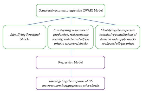
This paper investigated the response of US macroeconomic aggregates to price shocks in crude oil and natural gas markets using a two-step approach: firstly decomposing the price shocks to identify the structural shocks using a structural VAR model, and secondly, showing the response patterns of macroeconomic aggregates corresponding to each structural shock using a regression model.

Our main findings in this study are threefold. First, we found that there was a difference in the effects on real economic activity due to precautionary demand shocks from crude oil versus natural gas. Second, the cumulative contribution of oil-specific demand shocks to real oil prices is larger than the cumulative contribution of gas-specific demand shocks to real gas prices. Third, precautionary demand shocks had different effects on CPI inflation, depending on whether they were due to crude oil or natural gas. Therefore, economists, policymakers, and investors must decompose real prices of these important energy sources that have such significance in the economy and our daily lives. Finally, the most noteworthy of our findings is that oil market-specific demand shocks lead to statistically significant increases in the US CPI level, however, gas market-specific demand shocks barely affect the US CPI level. This result implies policymakers should react differently to gas-specific demand shocks and oil-specific demand shocks.

The similarities and differences between our empirical results and those of Kilian [6] can be summarized as follows. Firstly, comparing the results which showed the responses of global oil/gas production, real economic activity, and the real price of oil/gas to structural innovation reveal that they are alike with minor differences. The major distinction is the different effects on real economic activity that result from precautionary demand shocks to crude oil versus natural gas. Another point is that the statistically significant lasting period of influence from oil-specific demand shocks on global economic activity were shorter than they were prior to 2009, as the results from Kilian [6] showed. Secondly, comparing the results of the historical decomposition of real prices, our results for crude oil are approximately similar to Kilian, but one concern is that, during the period 1985–2000, Kilian’s study showed a negative cumulative effect of an aggregate demand shock on the real price of crude oil, while the effect in our study was extremely close to zero [6]. Thirdly, comparing the result of effects of respective shocks on the US macroeconomy, the empirical results are very similar with minor differences. The results of oil supply shocks on GDP showed that the two standard error bands were statistically significant for only half a year, compared to the two years reported in Kilian [6], which was explained by the one standard error band. Because of the different adoption of the standard error band, unanticipated oil-specific demand shocks led to a statistically insignificant reduction in US real GDP for all observed time horizons, whereas Kilian’s results implied statistical significance in the 3rd year [6].

Compared to previous literature, namely Zhang et al. (2017) [13], the similarities and discrepancies should be noted. Because not all natural gas price shocks cause GDP to decrease and the CPI to increase, when natural gas price increases originate from increasing uncertainty of the energy market, GDP would decline, and the CPI would rise. However, when natural gas price shocks are due to exogenous supply shocks, GDP would not always decrease, while the CPI would decline, which is a different outcome from that relating to aggregate shocks and specific demand shocks.

In this paper, the empirical evidence may have some implications for economists, policymakers, and investors albeit their self-evidence. Because our empirical results showed that the response patterns vary depending on the causes of the price fluctuations, not only for the crude oil market, but also the natural gas market, economists should take this into account when they construct their models for researching about oil/gas price shocks. Regarding the policy-making implications, especially for government monetary authorities such as central banks, there is a need to identify the underlying determinants that drive the price increases to make appropriate policy. For example, when the oil or gas price increase stems from an exogenous supply shock, there is almost no need to undertake any countermeasures because these kinds of shocks have a minimal effect on the macroeconomic aggregates. In contrast, with supply shocks, in which the price increases because of surging uncertainty in the oil market, thereby stimulating an increase in precautionary demand, monetary authorities should consider whether countermeasures should be undertaken to retard ongoing inflation; there is almost no need to take such countermeasures into account in the case of the gas market. Another implication concerns aggregate demand shocks: policymakers should distinguish where the aggregate demand shocks originated i.e., the crude oil market or the natural gas market. If the source of the shock lies in the oil market rather than the gas market, the corresponding responses should take into consideration prevention of a reduction of the GDP level over the long-run. As for the long-term investment implications, firstly, the investors must distinguish the origins of the oil/gas price fluctuation because the response pattern of each shock is different and requires distinct investment adjustments. Secondly, investors should pay attention to global aggregate demand shocks, and the specific demand shock rather than supply shocks, when they reconsider their investment structure, because precautionary demands shocks make a greater contribution to real price fluctuations than exogenous supply shocks. Because of developing environmental awareness, the demand for natural gas is gradually increasing and growing in importance in energy markets, thus implying that investors should take natural gas as an alternative investment choice for their portfolio adjustment when turbulence occurs in crude oil markets.

Despite our findings, this investigation has several limitations. First, the range of the dataset of natural gas prices is from 1994, which makes it impossible to compare the cumulative effect of demand and supply shocks between crude oil and natural gas during the period 1973–1993. Second, we adopted the Kilian Index (Kilian [6]); however, whether the Kilian Index is an adequate reflection of overall economic activity after 2009 is beyond the scope of this study. Because the driving forces and factors which influence global economic activity may have changed after 2009, there may now be a more appropriate index. Third, as mentioned above, during the period 1985–2000, Kilian’s study showed a negative cumulative effect of an aggregate demand shock on the real price of crude oil, while the effect in our study was extremely close to zero. The proper explanation for this outcome remains unknown and requires further research.

Therefore, in our future research, first, we plan to identify a more appropriate index to reflect overall global economic activity, and compare the results with those based on the Kilian Index. Second, as noted in Section 3.1.3, the cumulative contribution of an oil-specific demand shock to real prices is larger than the cumulative contribution of a gas-specific demand shock. Thus, we intend to identify the underlying determinants or causes of this issue. Third, in order to effectively apply our results to the policy-making process and inform appropriate monetary policy, we propose to extend the results by a machine learning approach to forecast price fluctuations corresponding to various kinds of uncertainty conditions, namely financial crises, wars, emergencies, disasters, etc. Fourth, the approach of Kilian [6], followed herein, did not include analysis of cointegration; thus, we plan to expand the analysis within the framework of cointegration. Finally, assessing the effects of oil/gas price shocks on other major countries’ macroeconomic aggregates is also worthy of extending the current investigation in future research.