Modelling of Polymeric Shell and Tube Heat Exchangers for Low-Medium Temperature Geothermal Applications

Abstract

Improvements in using geothermal sources can be attained through the installation of power plants taking advantage of low and medium enthalpy available in poorly exploited geothermal sites. Geothermal fluids at medium and low temperature could be considered to feed binary cycle power plants using organic fluids for electricity “production” or in cogeneration configuration. The improvement in the use of geothermal aquifers at low-medium enthalpy in small deep sites favours the reduction of drilling well costs, and in addition, it allows the exploitation of local resources in the energy districts. The heat exchanger evaporator enables the thermal heat exchange between the working fluid (which is commonly an organic fluid for an Organic Rankine Cycle) and the geothermal fluid (supplied by the aquifer). Thus, it has to be realised taking into account the thermodynamic proprieties and chemical composition of the geothermal field. The geothermal fluid is typically very aggressive, and it leads to the corrosion of steel traditionally used in the heat exchangers. This paper analyses the possibility of using plastic material in the constructions of the evaporator installed in an Organic Rankine Cycle plant in order to overcome the problems of corrosion and the increase of heat exchanger thermal resistance due to the fouling effect. A comparison among heat exchangers made of commonly used materials, such as carbon, steel, and titanium, with alternative polymeric materials has been carried out. This analysis has been built in a mathematical approach using the correlation referred to in the literature about heat transfer in single-phase and two-phase fluids in a tube and/or in the shell side. The outcomes provide the heat transfer area for the shell and tube heat exchanger with a fixed thermal power size. The results have demonstrated that the plastic evaporator shows an increase of 47.0% of the heat transfer area but an economic installation cost saving of 48.0% over the titanium evaporator.

1. Introduction

Climate change, rising pollution, and the fossil fuel depletion encourage many countries to push towards renewable-based energy conversion systems [1]. In particular, the European Union energy policy gives a high priority to the increasing use of renewable energy sources (RESs), because of their strong contribution to the diversification of energy supply, the improvement of the security of energy systems, the minimization of greenhouse effects and social and economic cohesion. In 2014 the European Union (EU) agreed to implement strategies and targets (revised in 2018) to move toward a low carbon economy. One of the pillars of EU policy in energy and environmental matters consisted of the RESs share increase in final energy consumption by at least 32.0% in 2030 compared to the 1990 level [2]. The attainment of the EU renewables target is ensured by the governance system based on national and local energy planning. Indeed, in recent years, it can be observed that a proliferation of ambitious commitments and policies in the RESs field adopted by national, regional, and local governments aimed to achieve EU goals [3]. Moreover, the support policies and strategies offer useful instruments to encourage renewable energy use and to ensure the full exploitation of RES’s potential in territorial areas where the energy policies’ actions are in force [4].

According to Eurostat [5] renewable energies covered 17.5% of final EU energy consumption in 2017. It has been estimated that the main renewable energy options which will contribute to the additional EU potential in 2030 are: wind power (239 TWh), transport biofuels (218 TWh), solar thermal in industry and buildings (117 TWh), biomass in industry and buildings (105 TWh), and solar photovoltaic (93.0 TWh) [6]. Unfortunately, the widely used and most promising RESs (such as solar and wind) are not programmable. Their availability varies throughout hours and seasons and, as a consequence, their use has to be accurately designed in conjunction with management strategies such as load shifting and energy storage. Thus, one of the possible pathways to mitigate the criticalities of this uncertainty is the exploitation of more flexible and stable RESs such as geothermal and biomass energy sources. In particular, geothermal energy is an abundant renewable source with significant potential. The geothermal reservoirs could be employed in direct use such as in district heating systems, in indirect use to produce electricity, and in cogeneration systems for the combined production of power, heating, and cooling energy [7]. The hot water reservoirs in low deep sites are used for direct scopes and/or district heating systems. Native American, Chinese, and Ancient Roman people adopted hot mineral springs for cooking and bathing; currently these could be used for thermal scope, heating, and domestic hot water. Geothermal energy provides heat requirements to buildings by means of district heating systems. Surface hot water is directed to buildings in the intermediate circuit. For example, in Reykjavik (Iceland), a district heating system supplies thermal energy to most of the buildings. On the other hand, the use of geothermal energy in industrial fields concerns gold mining, food dehydration, and milk pasteurizing. One of the most widespread industrial application of geothermal energy is represented by the dehydration of vegetables and fruit drying [8]. As concerns the electricity production from geothermal sources, traditional geothermal power plants exploit steam or water at high temperatures (150 to 370 °C). Geothermal power plants are usually located near reservoirs within one or two miles of the Earth’s surface.

Otherwise, geothermal sources are mostly available worldwide at medium and low enthalpy. In past years, geothermal energy has primarily been used in zones with a volcanic activity where there was a near sub-surface heat availability. Whereas, in recent decades geothermal energy usage has spread in many regions of the world thanks to the possibility of drilling to depths of several kilometres. In developed countries geothermal energy supply is especially widespread due to their flourishing economic means and industrial advances, as well as their availability of know-how and expertise. Besides, geothermal energy can be useful in developing countries to solve the energy access problems [9]. In Asia, only China owns 8.00% of world’s geothermal resources and it has 27.8 MW of geothermal installed power generation [10]. In Canada and Australia there is a large availability of geothermal resources at 100 °C near the land surface [11,12]. In South Africa (Main Karoo Basin region) a geothermal potential has been recently addressed, finding a geothermal gradient ranging from 24.5 °C/km to 28.2 °C/km at 3500 m depth [13].

On the other hand, in many countries geothermal sources have remained unused because of the acceptability problems of geothermal installations. Meller et al. [14] have identified the precondition for public acceptability of geothermal power plants, and they have analysed the social response to novel geothermal activity. The aim of their study has been to develop technological and scientific options by means of sociological studies for the responsible use of geothermal resources. Indeed, the participation of the public into geothermal projects should go further with communication and awareness-raising measures. By respecting the research rules and the development steps of technological solutions it is necessary for an open approach aimed to include governance structures. In some European countries (such as Germany, France, and Italy) the social response to geothermal projects evidences the reticence of the public and relevant stakeholders to eventual geothermal development in all considered countries. In addition to these issues, the high cost of geothermal installations and the regulatory uncertainty have jeopardized the diffusion of energy conversion systems based on low and medium enthalpy geothermal sources.

This is an Italian case in which the massive presence of geothermal sources (at high, medium, and low temperatures) is not completely exploited even if its potential has been recognised since the 1980s [15]. Interesting geothermal areas had been found in the southern Alps region at a temperature of 80–120 °C and a depth of about 3000 m [16]. In the transition zone between the chain and the basin of the Po plain, a certain heat flow anomaly (80.0 mW/m²) attributable to a geothermal gradient has been discovered. This heat flow is 21.3% higher than the Italian heat flow mean value (63.0 mW/m²) [17]. Moreover, a great heat flow anomaly affects the Mediterranean and central/southern Tyrrhenian Sea (>150.0 mW/m²). Intensive volcanic activity occurs on the Aeolian and Pantelleria islands (in Sicily) and in the Phlegraean Fields area (near Naples, South of Italy), resulting in geothermal fluid temperatures of 100–150 °C located near the Earth’s surface [18]. Despite this large availability, the only Italian geothermoelectric power plants are installed in Tuscany, characterised by high-temperature geothermal sources covering a power equal to 915 MW. These power plants are all traditional flash steam technologies that can use only geothermal high temperature fluids letting the low-medium resources go unused [19,20].

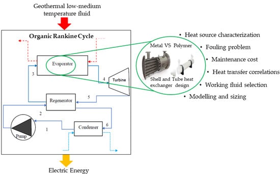
The major possibility of employing the low-medium enthalpy reservoirs for geothermoelectric applications is represented by binary cycles such as the Rankine Cycle with organic working fluids (ORC) [21]. Its layout is the same as an ordinary Rankine cycle, with the main difference being that in the ORC an organic fluid is used instead of water. The liquid-vapour phase change of an organic fluid occurs at a temperature lower than the phase change of water-steam, allowing for the use of low-medium temperature sources. In addition, the use of an organic fluid results in further advantages related to the thermo-physical proprieties of the fluid. The major used fluids in ORC systems are characterized by a positive slope of the vapour saturation curve which permits the avoidance of both superheating at the inlet of the turbine and condensation during the expansion process.

Among the different sources for an ORC, the most used and promising are biomass, sun, geothermal brines, and exhaust gases from industrial processes and engines. ORC plants can be characterized by their wide size range from a few kW_el (in residential cogeneration applications) up to tens of MW_el (in large power plants uses). As regards geothermoelectric plants based on ORC systems, worldwide only 16.0% of geothermal power plants are based on ORC technology such as those in Italy [21]. In particular, ORC power plants activated by geothermal sources number about 337, and these represent 19.2% of total ORC plants feeding by different sources. Geothermal ORC power plants cover 2021 MW_el representing 74.9% of the total power installed for the ORC systems. These data highlight that the geothermal ORC plants have higher size than other ORC plants fed by different RESs, and their medium power is 6.00 MW_el for a single plant [22].

The rising interest in ORC power plants is demonstrated by several works conducted in recent years to investigate their performances in different applications.

In [23,24] a binary ORC power plant for the use of medium-low enthalpy geothermal reservoirs is analysed firstly in a thermodynamic investigation/optimization, and secondly from an economic aspect. In [23] a Matlab code is defined to find the optimal match cycle parameters, configuration, and fluid taking into account geothermal waters in the temperature range of 120–180 °C. Thermodynamic optimization results show that the highest plant efficiencies are obtained for fluids that present a range of 0.88–0.92 of the ratio between critical working fluid temperature and inlet geothermal temperature and a supercritical cycle with a reduced pressure between 1.10 and 1.60 bar. Meanwhile, in the economic optimization these values are slightly lower and the advantages of supercritical cycles usage are less present.

In [24] an ORC powered by diesel engine waste heat recovery with different selected working refrigerant fluids such as R123, R134a, R245fa, and R22 is modelled and optimized. The optimization results, conducted by means of a genetic algorithm, show that the R123 is the best working fluid in both an economical and a thermodynamic sense for a defined value of output power. The optimum result of R123 determines the 0.01%, 4.39%, and 4.49% improvement for the yearly cost compared to R245fa, R22, and R134a, respectively. As regards thermodynamic optimization, the percentages of efficiency increase using R123 and other fluids (R245fa, R22, and R134a) are 1.01%, 12.79%, and 10.6%, respectively.

Regarding the geothermal applications of ORC systems, many studies have been aimed to assess the performance of the cascade geothermal plants based on ORC systems [25], and the performance of this technology through numerical [26,27,28,29] and experimental [30] works has been evaluated.

The cascade geothermal plants based on ORC systems coupled with other components, such as absorption heat pumps and heat exchangers for heat recovery, were analysed in many studies. In [25] Pastor-Martinez et al. have compared different polygeneration systems activated by low and medium geothermal sources (80–150 °C). The systems consist of an ORC (to produce electricity), an absorption heat pump (to provide cooling energy), and a heat exchanger (for heat recovery) arranged in different cascade configurations, with parallel or series geothermal fluid use. The study considers two possible plants in two different temperature ranges. For the first case, from 80 to 111 °C, the polygeneration arrangement presents the highest exergetic performance in the hybrid arrangement for parallel-series configuration, and it reaches the exergy efficiencies varying from 42.8% to 50.1%. Instead, the second one ranges from 110–150 °C, and awards a series cascade configuration achieving exergy efficiencies from 51.4% to 52.9%. In [26,27,28] other simulation studies integrate the desalinization water system to improve the polygeneration system layout using the geothermal fluid in cascade allowing a re-injection of the fluid at a lower temperature. The hybrid multi-purpose plant consists of an ORC powered by a low-medium temperature geothermal source and by solar energy from parabolic collectors. The geothermal water is first employed to activate the ORC loop, then to supply heating needs at about 85–90 °C (in winter), or space cooling (in summer) using a single-effect absorption chiller. At the end of the cycle, the geothermal water is used to feed a multi-effect distillation system. In this process the seawater is turned into freshwater. The results determine an energy efficiency of the ORC plant equal to 11.6% and a simple payback of 4.47 years. Another simulation study [29] is based on a zero-dimensional model of an ORC that allows for the investigation of the effects on the main output parameters (heat exchangers efficiency, ORC power output, ORC first law efficiency) by only changing the heat transfer coefficients correlations of the vapour generator available in literature. Two ORC plants both activated by a medium-temperature geothermal source supplying a constant thermal load are analysed in the study. The first case study regards an ORC module with a size of 1.20 MW_el fed by a geothermal fluid with a temperature of 160 °C and 7.00 bar and using n-pentane. The second ORC plant uses R245fa providing 8.00 kW_el and it is activated by a geothermal fluid at 95.0 °C and 3.00 bar. The first plant shows an electric efficiency of about 14% for all correlations investigated, while the second plant obtains an electric efficiency ranging from 7.00–10.0%. In [30], a real ORC plant in Huabei (China) shows the possibility for providing geothermoelectric energy from different thermal fluids in an aggressive environment. The plant with 500 kW_el employs fuel oil from an abandoned well using an intermediate circuit with an efficiency between 4.00–5.00% and consequently the output power of the turbine varies from 160–60.0 kW_el.

Even if ORC technology is very promising in low enthalpy geothermal applications, it is affected by a problem common to all technology exploiting geothermal sources. Geothermal fluids are often very aggressive (depending on geothermal sites) and they cause surface fouling, corrosion, and scaling over the heat exchanger (HEX) surface in which the heat transfer occurs through the working fluid evaporation. The scale formations threaten the heat transfer between geothermal and organic fluids, and they have also an impact on HEX performance in terms of flow velocity and pressure drop. Thus, they force the plant to turn off in order to clean or replace the HEX [31,32,33]. This issue causes an operating cost increase; indeed, it has been estimated that the impact of the HEX cost on the total plant investment costs ranges from 20.0% to 30.0% [34]. The HEX used in an ORC system is traditionally a metallic shell and tube type heat exchanger that has a high cost and low resistance to corrosion [35]. In [36] a mathematical model of the shell and tube heat exchanger (STHEX) is proposed for the capture and predicting fouling trends on both the shell and tube sides. The literature review is typically focused on fouling inside the tubes, and instead fouling on the shell side is not usually considered. In this work, instead, it has been demonstrated that fouling deposition on the shell side may be significant. It determines the not-equal heat transfer, growing pressure drops, and flow path modifications. Different solutions have been investigated to solve the fouling problems.

In [37] a study has been conducted to improve the corrosion-erosion features of carbon steel by using a multilayer composite coat for carbon steel plates. This solution is adopted to obtain better tribological behaviours and a lower wear rate of coatings than the untreated steel. In this application the nickel is linked with chromium to form Cr₂O₃ which allows us to use the material until 1200 °C. In particular the material use is ensured for temperatures lower than 800 °C thus, it could be used in both geothermal plant components and gas combustion applications. These coatings, however, produce very dense layers with a porosity under 0.500–1.00%. In [38] the performance of the HEX ceramic prototype has been evaluated. It is able to achieve a heat transfer of up to 6.00 kW and an effectiveness of up to 97.0%. It could operate at high temperatures and in harsh environments exceeding also the performance of a comparable metal HEX.

Another alternative path that can be followed is the replacement of the metallic HEX in geothermal ORC with a plastic (polymer) heat exchanger (PHEX). Indeed, a PHEX in ORC systems activated by geothermal sources ensures a higher inhibition of the scale depositions and the corrosion resistance limiting the maintenance periods for chemical or mechanical and/or hydrodynamic washing affecting the carbon steel HEX. Moreover, PHEX investments and maintenance costs are lower than those of a HEX with the same useful life cycle. Even if it is possible to consider the advantage of a PHEX for aggressive environment applications it is necessary to underline that the market for these components is thin for high working temperatures and pressures. The low operating temperature is compatible with geothermal sources, but the low pressure of exercise is not performing for organic fluids used in ORC systems. Thus, some advances are still required for the widespread use of plastic heat exchangers, but great improvements are expected in their market to justify the investigation on PHEX performance in innovative applications such as in ORC plants. This is the main topic of this work and in the following section the available literature information regarding PHEXs operating and design conditions in comparison with HEXs have been collected and summarised; in addition, the motivation and aims of the paper have been discussed too.

2. Polymeric Heat Exchanger: State of Art and Aim of the Study

Currently, the used materials for HEXs are metallic alloys, such as 70.0% Cu, 30.0% Ni, or titanium, with high thermal conductibility but with high corrosion and fouling resistances, especially in aggressive environments [39,40]. The types of fouling occurring in a HEX could be different, such as the precipitation of solid deposits in a fluid on the heat transfer surfaces (that can be cleaned by chemical treatment) or corrosion and other chemical fouling. The growth of algae in hot fluids can be a cause of contaminations in the heat exchangers. The biological fouling that the algae may determine can be avoided by chemical techniques. Moreover, in geothermal applications, the chemical aggressive composition of geothermal brines (strictly depending on geothermal site) determines the fouling on the HEX’s surface. All these problems cause the deterioration of material, the worsening of heat transfer efficiency, the increase of pressure losses due to friction, the reduction of crossing flow section, and the need for HEX replacement and cleaning. As a consequence, it may be necessary to employ a larger, and thus more expensive, HEX to achieve the required heat transfer performance when fouling takes place. All of these categories of fouling can be reduced by using plastic pipes instead of metal ones or by coating metal pipes with glass. Regarding polymer heat exchangers, their main advantages are: low cost, low weight, anti-corrosion, antifouling, manufacturing simplicity, electrical insulation, high chemical resistance, high modelling, and excellent elasticity (depending upon the working temperatures) [41,42]. The low PHEXs’ costs result in a decrease of up to 20% on power plant investment costs in which a titanium HEX evaporator is replaced by a PHEX one by considering the same life cycle [34]. Thus, the PHEX’s opportunities are evident in small-size applications and when the specific unitary cost is high. Indeed, with reference to a metal HEX’s cost in Figure 1, the investment cost of a common metal HEX against its heat transfer area is plotted starting from data available in literature for different heat exchangers’ geometries [43]. In Figure 1, the x-axis is stopped at 120 m² because it is the maximum size of the heat transfer area for the plate heat exchanger available from the market data comparable to other models. In addition, a HEX’s maintenance cost for 20 years of its life cycle is equal to 10.0–11.0% of the initial investment. Therefore, PHEXs offer an interesting alternative to the high cost of metal heat exchangers concerning both the investment and the maintenance costs, especially in aggressive operating conditions.

Another advantage of PHEXs is that they are already available on the market in multiple polymeric plastic materials (such as Ethilene Chloro TriFluoroEthylene (ECTFE); polyEthylenete TetraFluoroEthylene (ETFE); polyEthylene of high and low density (PEHD/PELD); PolyVinilChloride (PVC), etc.) and different manufacturing companies already produce PHEX worldwide: TMW (La Serre, France) [44], Polytetra (Bietigheim-Bissingen, Germany) [45], Aetna plastic (Valley View, United States of America) [46], HeatMatrix Group B.V. (Geldermalsen, Netherlands) [47], Fluorotherm (Parsippany, United States of America) [48], Ametek (Berwyn, United States of America) [49], Kansetu (Osaka, Japan) [50], and Calorplast (Krefeld, Germany) [51]. The most widespread geometries of PHEXs produced by the aforementioned companies are plate and shell and tube heat exchangers; only in particular cases is it possible to find immersion, hollow plates, or tube plate PHEXs. In addition to these benefits, PHEXs show also some critical issues that can be summarised as follows [52]:

• the most relevant parameter for HEXs’ design is the global heat transfer coefficient (UA) that takes into account the convective, conductive, and fouling resistances. The plastic thermal conductivity is usually equal to 1.00% of the thermal conductivity of metallic materials [53,54]. This fact determines a penalization of the heat transfer performance; thus, a higher heat transfer surface area is requested.
• the PHEX has low structural strength and poor stability in terms of mechanical resistance at high temperatures or pressures. Indeed, the limits of PHEXs are the working couple of pressure and temperature that the material can support. At high temperatures, the maximum operating pressures of the commercial devices are often incompatible with the operating pressures of organic fluids defined for ORC market applications [34].

  Table 1. Operating temperatures and pressures for different polymer materials.

  Plastic Materials	Working Temperature (°C)	20	40	60	80	100	120	140
  PFA	Rupture pressure (bar)	59.98	47.99	38.96	29.99	19.99	12.00	6.00
  	Max working pressure (bar)	10.00	8.00	6.48	5.03	3.52	2.00	1.03
  PVDF	Rupture pressure (bar)	79.98	55.02	49.99	39.99	29.99	22.41	17.44
  	Max working pressure (bar)	12.00	10.00	7.52	6.00	4.48	3.52	2.96
  PP/PE	Rupture pressure (bar)	24.96	18.00	14.00	8.00	-	-	-
  	Max working pressure (bar)	8.00	6.00	4.00	2.00	-	-	-

  shows a summary of the optimal working temperature and pressure values for each plastic material available for shell and tube exchangers. It is important to underline that the maximum operating temperatures could be higher when the pressure is reduced and vice versa. In general, it should be noted that the materials most resistant to high temperatures (>100 °C) are Perfluoroalkoxy alkanes (PFA) and polyvinylidene difluoride (PVDF) which, however, have lower thermal conductivity (about half) than PE and PP. The limit for the PE polymers is under 100 °C for the hot fluid considered. Over this value of temperature, it is necessary for the use of a polymer with a higher mechanical resistance. In particular, from market analysis, it has been found that it is easy to reach operating temperatures close to 100 °C by improving the composition of polymers; for example, by adopting high density PE (PEHD) as suggested by the manufacturer [51].

PHEX’s problems have been investigated by researchers in recent years by means of simulative and experimental applications. For instance, in [55] the authors have demonstrated through an experimental analysis that PHEXs conductive resistance (that is proportional to the inverse of thermal conductivity) amounts only to 3.00% of the total thermal resistance (including fouling, convective, and conductive resistance). Moreover, the percentage weight of conductive resistance on total thermal resistance is strictly linked to the value assumed by convective and fouling resistances which depend on many factors such as the thermodynamic condition of the fluid and the Reynolds numbers (by velocity definition) of the fluid that crosses the PHEX [56]. Other authors have found that an enhancement of the polymer heat transfer coefficient can be obtained by filling the polymeric matrix with high conductivity additives or by controlling its crystallinity [57]. In support of these theories in [58] it is experimentally shown that the specific volumetric heat transfer coefficient of a PHEX in polyamide filled with carbon fibres is 1.65 times higher than that produced with a polyamide only. On the other hand, even if polymers constituting PHEXs have a low mechanical resistance, they can deform elastically meaning that they return to their original form after thermal or mechanical stress. Moreover, PHEXs’ low structural strength results in a light weight. Indeed, in [59] it has been estimated that the metal HEXs have many drawbacks related to their weight, and PHEXs ensure up to 62.2% of weight reduction.

PHEXs’ applications have been recognised as particularly suitable in different fields as seawater heat exchangers, solar water systems, heat recovery applications, and for the desalination industry in a corrosive environment [60]. PHEXs can also represent a good solution for ORC applications, since ORC systems are characterized by aggressive/low temperature heat sources and a high specific cost, so the heat exchanger’s cost has a great weight in the overall cost of such technology. Despite this opportunity, there is a gap in the literature review concerning the PHEX use in ORC exploiting geothermal brine. To the best of authors’ knowledge, only Gomez et al. [34] have conducted a simulative analysis to investigate the possible replacement of a titanium HEX with a PHEX in low size Organic Rankine Cycles for geothermal applications to reduce plant investment costs. They have conducted a thermodynamic analysis of a 20 kW_el RORC plant according to the currently available data on market for shell and tube PHEXs. Then, the authors compared a PHEX and a metallic HEX from an economic point of view finding that for a plant availability for 5000 h of functioning in a year and a discount rate of 10%, a cost of the generated electricity equal to 94.8 $/MWh for a plastic solution and 118.9 $/MWh for a titanium HEX can be obtained.

In this context, the main aim of this work is to determine whether it is possible to employ PHEXs as an alternative to conventional metallic HEXs in an ORC-based plant using a geothermal source. The work wants to define the advantages and disadvantages of HEX replacement considering the main design proprieties, such as the heat exchanger’s surface area, the overall heat exchange coefficient, and also economic aspects. The novelty of this work concerns the development of a one-dimensional mathematical numerical model of a polymeric STHEX based on discrete elements for geothermal ORC applications. Thus, unlike other works in the literature review, PHEX is not modelled as a “black-box” accounting only for the inlet and outlet fluids’ operating conditions, but the heat transfer inside tubes is modelled considering PHEXs’ conductive, convective, and fouling resistances too. The study is based on a MATLAB algorithm with a REFPROP interface able to provide the value of design characteristics such as the heat transfer area, the length of tubes, and the heat transfer coefficient in a shell and tube heat exchanger configuration. A sensitive analysis is carried out varying the inlet temperature of geothermal brine using literature correlations in the worst fouling condition.

3. ORC Configuration with PHEX in a Geothermal Plant and Working Fluid Selection

The most common applications provide the use of a STHEX in geothermal ORC systems because it can be cleaned easily. Among all heat exchangers, STHEXs are the most widespread heat exchangers covering 65.0% of the market in different applications [61]. The common practice considers the allocation of fluids with the maximum predisposition to scale in the side of tubes to facilitate the cleaning of the component. However, the fluid on the side of the shell can also be subjected to fouling. In such cases, the neglect of fouling effects in the shell-side may lead to great errors in the analysis of the data [36]. In this paper a shell and tube PHEX is considered as an evaporator in a geothermal ORC plant. The possibility of component cleaning is neglected due to its higher fouling resistance, whereas it is considered with the opportunity of PHEX replacement according to its low cost. Thus, this work considers the organic fluid flowing inside the tubes and the geothermal hot brine is confined in the shell, resulting in a counter-cross flow heat exchanger. This choice leads to two advantages:

• it is more economically convenient to build high pressure pipes (in which the organic working fluid with the higher pressure is flowing) than the high-pressure shell [56];
• the pipe-side heat transfer coefficient is superior to shell side coefficient thanks to the presence of boiling organic fluid in the pipes [62].

The considered plant, in a regenerative ORC configuration (RORC), is represented in Figure 2. It is composed of a pump, turbine, regenerator, condenser, and evaporator that provides the interaction between the two fluids: the hot vector fluid (geothermal brine) and the organic working fluid. Geothermal fluid is taken from the aquifer and then it is pre-treated. The geothermal fluid considered in this work refers to the Phlegrean Fields area (south of Italy). The choice of the hot fluid temperature derives from a previous analysis conducted by Carlino et al. in [63] from which it has been possible to evaluate the geothermal gradient. By analysing the census relating to the area of interest an average value of the well surface temperatures has been considered excluding temperatures below 70 °C (temperature typically used for reinjection). The temperature of the pre-treated hot resource used in this analysis is about 95 °C, compatible with the ORC manufacturer data request [64]. In particular, the Phlegrean Fields area is heavily affected by medium-low enthalpy geothermal sources [65]. It has been demonstrated that near Pozzuoli there are many zones interested by geothermal source availability with a temperature near 90 °C. Different studies have typically analysed the chemical composition of geothermal fluid at high deep sites and temperatures (~200–300 °C) [63,66], and have also presented data on flow rates and tempering available in the Campania region such as the geothermal brine chemistry characteristic. Furthermore, few literature data show the chemical composition at lower temperature conditions despite the studies evidencing the high variability of the geothermal source in Campania. However, in the Phlegrean Fields area the geothermal sites show various temperature gradients (20–180 °C/km) and temperature profiles, different flow rates, and heat flow density (from 20 to 140 mW/m²) [67]. Some data about the chemical-physical composition of geothermal water at low temperatures in Phlegrean Fields are reported in

Table 2. Chemistry composition of geothermal fluid for low-medium temperature sources.

Geothermal Fluid Properties	H. Tennis #1	H. Tennis #2
T (°C)	88.9	85
ph (–)	7.41	7.2
TDS (ppm)	5390	-
Na+ (ppm)	1540	1295
K+ (ppm)	455	407
Ca2+ (ppm)	38.7	58.1
Mg2+ (ppm)	1.3	4.9
Sr2+ (ppm)	0.4	0.9
Li+ (ppm)	-	0.96
Rb+ (ppm)	-	1.41
NH4+ (ppm)	-	23.5
Cl– (ppm)	1536	1380
HCO3–(ppm)	753	699
SO42– (ppm)	1040	1136
F– (ppm)	-	3.5
SiO2 (ppm)	-	183.5
Al3+ (ppm)	-	0.5
B (ppm)	-	44.8

. The data derive from studies conducted in Phlegraean Fields before 1980 [68], during the period 1990–1999 [69,70]. In some of these studies information about the possible change in geothermal fluid composition and temperature after the bradyseism both in the fumaroles and thermal waters are reported. In addition, it has been evidenced that the shallow water system is locally activated by a deep hydrothermal element, generating in the form of boiling pools and wells the hot waters at the surface with temperatures around 90 °C. In Table 2 the chemical composition of geothermal fluids suitable for our simulation data set according to their temperature and chemical composition compatible with a heat exchanger and ORC considered system is reported. Both the columns (H. Tennis #1 and H. Tennis #2) are referred to H. Tennis well for two different periods [64,69]. Nevertheless other geothermal sites at low-medium temperatures are available in Phlegrean Fields, but because of their extreme sulfate and ammonium composition prevalence, higher presence of Fe and SiO₂, and extremely low pH, they are not considered [66,67,68]. In fact, they could require further analyses for numerical simulation because of their large quantities of silica, iron, aluminum, and sulfate could induce massive precipitations of minerals in the PHEXs. According to the literature the prevalent elements are Na, Cl, and total dissolved solids (TDS). In this work the geothermal fluid in the water dominated condition is simulated by using the REFPROP library which allows us to evaluate the thermodynamic properties of pure water. This approximation is endorsed by a previous analysis which allowed for the estimation of the variation of the thermodynamic properties of geothermal fluid with respect to pure water for the Phlegrean Fields site in the case of the temperature of the source at 94 °C. The results showed that the thermodynamic parameters variation (estimated by means of a software capable of integrating the salinity of the water) is not appreciable and, therefore, does not affect the hot fluid heat transfer coefficient. The geothermal brine aggressive chemical composition determines corrosion and depositions of suspension solid particles on the heat exchanger surface. In order to consider these disadvantages in heat transfer efficiency, the fouling resistances are included in the design methodology of the heat exchanger. In addition, fouling conditions are closely related to the depth of the extraction site, the withdrawal temperature, the dominant water or steam condition, and the thermo-physical characteristics of the fluid in the geographical area of interest. Therefore, the treatment that the geothermal fluid undergoes before entering the evaporator has not been simulated.

Regarding the organic fluid, a lot of works have been conducted to choose the best fluid with optimum thermo-physical, economic, and environmental properties in coupling with a low-medium temperature source [71,72]. In particular, the working fluid selection depends on the heat source temperature and the condenser cooling fluid temperature as well as on the ORC size. Some analyses show that the organic fluids characterized by high critical temperature allow for the obtainment of a higher ORC cycle efficiency, but this condition is verified only for the fluids with high reduced pressure. Indeed, the high critical temperature determines substantial expansion ratios and low condensing pressures making these fluids suitable for low-temperature applications [73]. Besides, they allow for the avoidance of the technical problems related to low evaporation pressure [74], the obtainment of an acceptable pinch point temperature difference [75], and low costs associated with the exergy destruction even if they are strongly influenced by the amount of working fluid used [76,77]. Moreover, the use of fluids with a molecular weight greater than that of water can improve the isentropic efficiency of the turbine and it may allow for the use of single-stage expander reducing the plant costs [78].

Thus, the pentafluoropropane (R245fa) is the organic fluid chosen in this application. It is suitable for different heat transfer applications such as low-temperature refrigeration, passive cooling devices, ORC for heat recovery, and in sensible heat transfer. The R245fa is useful for its special compatibility with widespread materials of construction as metals, elastomers, and plastics. It is also assessed for its good properties concerning human safety, health, and environmental aspects as toxicity, flammability characteristics, exposure limits, global warming potential, and safe product handling [79]. Calise et al. [80] have demonstrated that R245fa is the fluid with the best performance (in terms of heat exchange efficiency and environmental pollution) among other organic fluids in geothermal applications when geothermal brine temperature is lower than 170 °C.

The design of the PHEX is based on the manufacturer data of an ORC system available on the market [51].

4. Methodology

This section aims to elaborate a numerical algorithm for the shell and tube ORC evaporator design carrying out a comparison among different materials for HEX construction such as PEHD, carbon steel, and titanium. The model has been developed considering the nominal thermal power (${\dot{Q}}_{obj}$) of the STHEX provided by an ORC manufacturer [63]. The numerical model is based on physical equations developed in a MATLAB/REFPROP environment [81,82]. The physical equations presented here are equal for all the analysed materials while the parameters used in the equations vary from one STHEX material to another. Moreover, the correlations for evaluating the heat transfer coefficient used to determine the heat transfer rates are linked to the working fluid phase (single-phase or two phases) and to its position (shell or tube). The flow chart of the numerical algorithm developed and implemented in a Matlab code is reported in Figure 3. At the initial step the fixed parameters are allocated, and thermodynamic (

Table 3. ORC nominal data [63].

Parameters	Value
Critical Temperature R245fa (°C)	154.05
Primary Thermal Power (kWth)	450
Condensation water Temperature (°C)	33.0
Outlet Pressure Condensation (bar)	1.00
Flow rate working fluid R245fa (kg/s)	2.65
Flow rate geothermal brine (kg/s)	13.4
Inlet Evaporator Temperature hot fluid (°C)	94.0
Inlet Turbine Temperature working fluid (°C)	85.0
Outlet Turbine Temperature (°C)	60.0
Generator Cooling Water Temperature (°C)	<40.0

) and geometric (

Table 4. Shell and tube heat exchanger data.

Parameters	Symbol	Value
Inlet diameter tube (m)	di	6.00 × 10−3
Thickness diameter tube (m)	st	6.00 × 10−4
Shell diameter (m)	Ds	0.180
Shell limit diameter (m)	Dlimit,s	0.200
Max total length HEX (m)	Lt	6.00
Number of rows (-)	nrow	3.00
Number of tubes for each row (-)	nt,bank	117
Fouling resistance tube side (R245fa) (m2K/W)	Rt,f	1.00 × 10−4
Fouling resistance shell side (water) (m2K/W)	Rs,f	2.64 × 10−4

) parameters are assigned as well as the thermal conductivity variable for each investigated material. At the first step of integration (j = 1), R245fa temperature (T_t,o, tube side) is set equal to its outlet temperature indicated by constructor, while the temperature of hot geothermal brine (T_s,i) is set equal to the hot source temperature required from the evaporator (since the evaporator is a HEX in counter-flow configuration). The mass flow rates in the tube side ($\dot{{\mathrm{m}}_{\mathrm{t}}}$) and shell side ($\dot{{\mathrm{m}}_{\mathrm{s}}}$) are allocated too, according to values reported in Table 3. Then, in each iteration step the heat transfer coefficients (Equations (3)–(15)), the overall heat transfer coefficient (Equation (2)), and the elementary thermal power (Equation (1)) are evaluated. At step j+1, the geothermal brine temperature in the shell side (T_s (j+1)) and the specific working fluid enthalpy in the tube side (h_t (j + 1)) are evaluated. Enthalpy at the tube side is obtained from REFPROP software.

This procedure must be repeated until the heat power target is achieved (${\dot{Q}}_{obj}$). Finally, the total evaporator length L and the total heat exchanger surface (A) can be evaluated for each investigated material.

4.1. Model Equations

The proposed configuration for counter-flow STHEX is shown in Figure 4. The working fluid (R245fa) flows in the tubes (with a total length named L_t and a diameter called d_i) while geothermal hot water crosses the shell with a diameter indicated as D_s and a length called L_S.

The Matlab model is developed to define the STHEX area needed to obtain the fixed evaporator thermal power for each selected material.

The STHEX modelling depends on the following assumptions:

• steady-state conditions are considered for the the heat exchanger operations;
• the temperature of both working and hot fluids, at the exit and inlet of the section, is unvariant in the cross-sectional areas of the shell and the tube;
• the heat losses from the external heat exchanger surface to the surroundings are not considered;
• thermo-physical properties are integrated on a suitable infinitesimal element (dL) of tube with a fixed length of 5 mm;
• no variation in potential and kinetic energies of the flowing streams are taken into acoount;
• the plastic material able to withstand the operating pressures of the working fluid is considered;
• the pressure drops across tube side of heat exchanger are overlooked.
• the geometric condition fixes the tube banks rotated at 45°.

MATLAB model calculates the infinitesimal thermal power for each dL in every iteration using Equation (1). The calculation process stops when the sum of the infinitesimal thermal power ($\delta \dot{Q})$is equal to the nominal thermal power of the evaporator (${\dot{Q}}_{obj}$). The infinitesimal temperature difference (dT) between geothermal and R245fa fluids in each dL is evaluated using REFPROP library starting from two thermodynamic properties of fluids. The overall heat transfer coefficient (U) is evaluated as the reciprocal of the thermal resistance (R) in each dL defined as expressed in Equation (2).

$$\delta \dot{Q}=\underset{0}{\overset{\mathrm{L}}{{\displaystyle \int }}}\frac{\mathrm{dT}·\mathrm{dA}}{\mathrm{R}}\mathrm{dL}$$

(1)

$$\mathrm{U}=\frac{1}{\mathrm{R}}=\frac{1}{{\mathrm{R}}_{\mathrm{s}}+{\mathrm{R}}_{\mathrm{s},\mathrm{f}}+{\mathrm{R}}_{\mathrm{w}}+{\mathrm{R}}_{\mathrm{t}}+{\mathrm{R}}_{\mathrm{t},\mathrm{f}}}=\frac{1}{\frac{1}{{\mathrm{a}}_{\mathrm{s}}}+\frac{1}{{\mathrm{a}}_{\mathrm{s},\mathrm{f}}}+{\mathrm{R}}_{\mathrm{w}}+\frac{1}{{\mathrm{a}}_{\mathrm{t}}}+\frac{1}{{\mathrm{a}}_{\mathrm{t},\mathrm{f}}}}$$

(2)

Thermal resistance considers the convective heat transfer process in the tube (R_t) and shell (R_s) side, fouling in the tube (R_t,f) and shell (R_s,f), and conductive heat transfer through wall material (R_w).

The correlations used to calculate the resistances in the shell and tubes are described in the following subsections. Additionally, the fouling resistances both in the shell and tube’s side are constant and they depend upon the fluid.

4.2. Shell-Side Model Equations

The heat transfer convective coefficient into the shell side can be obtained considering the fluid in static condition assimilated to liquid water at a temperature range defined by the manufacturer. The convective coefficient for the shell side ${\mathsf{\alpha }}_{\mathrm{s}}$ depends on the Nusselt number (Nu), the diameter of shell (D_S) and thermal conductivity (${\mathrm{k}}_{\mathrm{s}}$) as reported in following Equation (3):

$${\mathsf{\alpha }}_{\mathrm{s}}=\frac{Nu·{\mathrm{k}}_{\mathrm{s}}}{{\mathrm{D}}_{\mathrm{s}}}$$

(3)

where the Nusselt number is calculated according to Equation (4) in laminar condition [83] and to Equation (5) for turbulent regime [84].

$$Nu=1.04·{\mathrm{Re}}^{0.4}·{\left(\frac{\mathrm{Pr}}{{\mathrm{Pr}}_w}\right)}^{0.36}$$

(4)

$$Nu=0.023·{\mathrm{Re}}^{0.8}·{\mathrm{Pr}}^n$$

(5)

In Equation (4) t Pr_w is the Prandtl number value on the wall. In Equation (5) n parameter assumes the value 0.300 if the shell side fluid is the cold one or 0.400 if it is the hot fluid. The Reynolds (Re) and Prandtl (Pr) numbers are defined as in Equations (6) and (7), respectively:

$$\mathrm{Re}=\frac{\dot{\mathrm{m}}·\mathrm{D}}{\mathsf{\mu }·\mathrm{A}}$$

(6)

$$\mathrm{Pr}=\frac{\mathsf{\mu }·c_p}{\mathrm{k}}$$

(7)

where $\dot{\mathrm{m}}$ represents the mass flow rate, D is the diameter, A is the area, $\mathsf{\mu }$ is the dynamic viscosity, c_p is the specific heat at constant pressure, and k the thermal conductivity. Generally, ${\mathsf{\alpha }}_{\mathrm{s}}$ is multiplied by a corrective factor J that considers different parameters such as the number of baffles and their configuration, dispersion, and losses in shells and deflectors, and losses in the nozzles and temperature gradients that could cause accumulations. The presence of the baffles which cut the diameter by 20.0%–45.0% allows for support and prevents vibrations and vortices in the pipes. In this work as suggested by the literature, J is equal to 0.60 [56].

4.3. Tube Side Model Equations

For the tube side of STHEX the organic working fluid (R245fa) chosen for the simulation is in phase-transition; therefore, it is not advisable to consider it as a liquid for all tubes length. It is necessary to distinguish if the fluid is in two-phase or single-phase condition for convective heat transfer coefficient (${\mathsf{\alpha }}_{\mathrm{t}}$) evaluation. In a single phase condition, the equation used is Equation (5). In a two-phase condition α_t corresponds to ${\mathsf{\alpha }}_{\mathrm{tp}}$ expressed by the correlation of Gungor-Winterton [85] reported in Equation (8). It takes into account two contributions: a convective boiling term (${\mathsf{\alpha }}_{\mathrm{cb}}$) and a nucleate boiling term (${\mathsf{\alpha }}_{\mathrm{NB}}$).

$${\mathsf{\alpha }}_{\mathrm{tp}}=\mathrm{S}·{\mathsf{\alpha }}_{\mathrm{NB}}+\mathrm{E}·{\mathsf{\alpha }}_{\mathrm{cb}}$$

(8)

where α_NB term is calculated from Cooper correlation [86] (Equation (9)):

$${\mathsf{\alpha }}_{\mathrm{NB}}=55·{\mathrm{pr}}^{0.12-0.2·{\log }_{10}\mathrm{Rp}}·{(-{\log }_{10}\mathrm{pr})}^{-0.55}·{\mathrm{M}}^{-0.5}·{\mathrm{q}}^{0.67}$$

(9)

M is molecular weight of the substance, pr represents the ratio between the operating pressure and critical pressure and q is the heat flow.

α_cb term in Equation (8) is calculated from the Dittus–Boelter correlation that is employed to calculate the heat transfer of liquid only in the tubes (Equation (10)) [87]:

$${\mathsf{\alpha }}_{\mathrm{cb}}=0.023·\frac{{\mathrm{k}}_{\mathrm{t}}}{{\mathrm{d}}_{\mathrm{i}}}·{{\mathrm{Pr}}_{\mathrm{t}}}^{1/3}·{{\mathrm{Re}}_{\mathrm{t}}}^{0.8}·{\left(\frac{{\mathsf{\mu }}_{\mathrm{t}}}{{\mathsf{\mu }}_{\mathrm{t},\mathrm{w}}}\right)}^{0.14}$$

(10)

where k_t is thermal conductivity, and μ_t and μ_t,w are the viscosity in the tube and wall, while Pr_t and Re_t are Prandt and Reynolds numbers, respectively, referred to the tube side as well, as k_t is the thermal conductivity of tube.

S (Equation (8)) shows the suppression factor of a nucleate boiling term that takes into account the decrease of fluid layer thickness as the vapour quality grows. E (Equation (8)) is the enhancement factor of the convective boiling process due to the increase of flow velocity when the vapour quality increases. The heat transfer coefficient is strongly and positively influenced by the vapour quality [88] and also by the frictional pressure gradient [89].

E and S factor are defined as in Equations (11) and (12), respectively:

$$\mathrm{E}=1+24000·\left({\mathrm{Bo}}^{1.16}\right)+1.37·{\frac{1}{{\mathrm{X}}_{\mathrm{tt}}}}^{0.86}$$

(11)

$$\mathrm{S}=\frac{1}{1+1.15·{10}^{-6}·{\mathrm{E}}^2·{\mathrm{Re}}_{\mathrm{l}}^{1.17}}$$

(12)

In Equation (12) Reynolds number is referred to liquid condition (l).

In Equation (11) two dimensionless numbers are considered: the Martinelli parameter (X_tt) and the Boling number (Bo) defined in Equations (13) and (14), respectively:

$${\mathrm{X}}_{\mathrm{tt}}=(\frac{1-\mathrm{x}}{\mathrm{x}}{)}^{0.9}·{(\frac{{\mathsf{\rho }}_{\mathrm{v}}}{{\mathsf{\rho }}_{\mathrm{l}}})}^{0.5}·{(\frac{{\mathsf{\mu }}_{\mathrm{v}}}{{\mathsf{\mu }}_{\mathrm{l}}})}^{0.1}$$

(13)

$$\mathrm{Bo}=\frac{\mathrm{q}}{{\mathrm{G}}_{\mathrm{t}}{\mathsf{\lambda }}_{\mathrm{l},\mathrm{v}}}$$

(14)

where x is the title, 𝜌_l, 𝜌_v are density in liquid and vapour condition, λ represents the latent heat and G_t is the flow rate in the tube.

4.4. Case Study

As before mentioned, the PHEX design is based on the manufacturer’s data of an ORC system available on the market that delivers 30.0 kW_el with a primary power input equal to 450 kW_th.

In Table 3 the ORC module parameters that were considered for the modelling and simulation analysis are reported.

The geometrical construction data of the STHEX are referred to the schedule of PHEX company and they are listed in Table 4, while in

Table 5. Thermal Conductivity of simulated Materials.

Material	kw (W/mK)
PE	0.510
Titanium	16.0
Inox Steel	20.0
Carbon Steel	47.0

the thermal conductivity of simulated materials (kw) are showed.

5. Results

The numerical algorithm has been employed with the aim of returning the heat transfer area (A) at the manufacturer’s conditions for each considered material. The evaporator area needed to provide the required electric output, for the simulated ORC system is higher in the case of plastic material with respect to the other ones. In particular, the increase percentage between A of PHEX and HEX in carbon steel amounts to 48.5%. The percentage decreases to 47.5% and 47.0% if the PHEX’s area is compared to area of a HEX made of inox steel and titanium, respectively. The difference among the area values is mainly due to the conductive and fouling resistance since the convective coefficients are similar for each material. In Figure 5 the values of the overall heat transfer coefficients and the heat transfer area of STHEX in plastic and metal materials are shown. As expected, PHEX provides the lowest value of U (88.5 W/m²K) and its contemporary needs the highest A (524 m²).

STHEX length and the heat transfer coefficient are summarized in

Table 6. Simulation results data.

STHEX Length and the Heat Transfer Coefficient	PEHD	Titanium	Inox Steel	Carbon Steel
L (m)	12.2	6.44	6.39	6.26
UA (W/K)	7.6	14.4	14.5	14.8

for all considered materials. The length as well as the heat transfer area (Figure 5) are evaluated by summing the values in each iteration step, while UA and U values are calculated in each iteration. Table 6 and Figure 5 average values of UA and U weighted on the infinitesimal area are listed, respectively.

The purchase cost (PC) evaluation for STHEX made of common steel materials (inox steel and carbon steel) is carried out by means of a literature correlation (Equation (15)) suitable for evaporators at high-pressure conditions [90]:

PC = 190 + 310 A

(15)

On the other hand, the evaluation of plastic and titanium STHEX costs have been conducted through a market analysis. The comparison is based on PC neglecting the maintenance and cleaning cost. In Figure 6 PCs for a PHEX (green bar) and metal materials (orange bars) are showed. The purchase cost of a STHEX in plastic material (27,597€) is significantly lower than a titanium STHEX (56,155€) while it is higher than a STHEX in inox steel (14,595€) and carbon steel (14,265€). Nevertheless, the economic comparison aimed to evaluate PC saving is relevant only between PHEX and HEX in titanium since in these two cases,the life cycle of two components are equal [91] and it is possible to neglect the cleaning cost for both STHEXs. Thereby, the percentage reduction of PC between PHEX and titanium STHEX is 48.0%. This reduction can have a significant weight for ORC plant investment costs since the unitary specific cost of the overall system is high.

In Figure 7 the convective heat transfer coefficient for the tube α_t, Figure 7a), for the shell α_s, Figure 7b) and overall heat transfer coefficient (U, Figure 7c) are shown as a function of heat exchanger length. These trends result from simulations in a MATLAB/REFPROP environment.

Since STHEX is in counter flow configuration, at L equal to 0 m (that represents the end of length integration) the geothermal brine is in inlet condition in the shell and the organic fluid is in the outlet condition of tubes side.

As reference to α_t (Figure 7a) at the integration start point of the evaporator (L = 0 m) the organic fluid in tubes is in satured vapour condition. Subsquently, α_t increases assuming a bell curve shape, and in this condition the organic fluid is in a two-phase state. As a matter of fact, in the two-phase condition the convective heat exchanger coefficient (α_cb) is characterized by two contributes (a convective boiling term α_NB and a nucleate boiling term α_NB) as reported in Equation (8). After that, α_t decreases and the curves becomes flat near the exit of the evaporator when the R245fais in the liquid condition (the condition of inlet state in STHEX) and the convective heat transfer coefficient is calculated through (Equation (10)). α_t curves for all metal materials have the same trend and are very similar; indeed, they are almost overlapping. α_t curve for plastic material has a larger bell, even if it shows the same trend of the metal materials’ α_t curves. For this reason, if an L value is assigned, α_t value in metal STHEXs is very different from the α_t value of PHEX (for example for L = 5 m α_t is equal to 4024 W/m²K and 3601 W/m²K for PHEX and titanium, respectively). α_s (Figure 7b) shows a decreasing trend and it is proportional to the geothermal brine temperature; therefore, during the fluid cooling the efficiency of heat exchange is down. At the evaporator integration starting point (L = 0) geothermal fluid has a high temperature, and so also α_s is high. Then it decreases with the increase of length for all materials. α_s stops at L = 12.2 m for PHEX because it is the needed length to ensure the required ORC electric output. In Figure 7 R_w, α_s,f, and α_t,f are not shown even if they are accounted for in the overall heat exchanger coefficient evaluation according to Equation (2). They are constant along whole STHEXs and they are calculated as following: R_w depends upon k_w of each material reported in Table 5, while α_s,f and α_t,f are the reciprocal of R_s,f and R_t,f evaluated for the geothermal brine and R245fa, respectively, according to values listed in Table 4. The overall heat transfer coefficient Figure 7) follows α_t trend for all materials since this term has the higher weight in Equation (2). Among metal materials the carbon steel STHEX has the highest U for a fixed L value since it shows the greatest k_w. PHEX has the lowest U for along whole evaporator.

Sensitivity Analysis

The Figure 8 reports the purchase cost and the needed heat transfer area value for a STHEX made of PEHD and titanium by varying the inlet temperature of geothermal brine in the range 94–99 °C. The temperature range for this sensitivity analysis is chosen considering the temperature availability of geothermal brine in selected sites and the possible operating couple temperature-pressure in polymeric heat exchanger applications. These values of inlet temperature allow the use of the same correlation (Equations (3)–(7)) for the shell side of the main case analysed. In Figure 8 the values in red points and red bars correspond to the inlet geothermal fluid temperature provided by the manufacturer (94 °C). The PC and the heat transfer area diminishes with the increment of inlet temperature of geothermal sources in both PEHD and titanium evaporators.

In particular, the reduction of the heat transfer area for each degree of geothermal brine inlet temperature increase is higher for the PEHD evaporator than the titanium one. Vice versa, referring to PC the cost reduction is more rapid for the titanium than the PEHD evaporator. For example, by going from T = 95 °C to T = 96 °C the reduction of PC amounts to 2633€ for PHED and to 5612€ for titanium. Considering the same temperature range, the heat transfer area reduction is equal to 8.4 m² for the PHED evaporator and 4.7 m² for the titanium STHEX. In particular, the installation of the titanium STHEX evaporator in an ORC plant is responsible of an extra-cost equal to 28,558€ with respect to the PHED one when the inlet temperature of geothermal brine is 94.0 °C. This extra-cost ranges from 25,578€ to 17,799€ when the inlet temperature changes in the range of 95.0–99.0 °C. On the other hand, the heat transfer area growth by using a PHED evaporator instead of a titanium one varies from 41.6 m² to 29.8 m², when the inlet temperature of geothermal fluid goes from 94 °C to 99 °C.

6. Conclusions

Organic Rankine Cycle technologies are employed worldwide in different fields. Among other applications, this work is focused on ORC plants using a geothermal source. Such systems are affected by different issues: a corrosive heat source, low exercise temperatures, and high specific costs, thus evaporator cost has a great weight on the overall plant costs. These problems can be making possible the using of plastic evaporators instead of traditional ones made of metal materials with a high cost and a low corrosion resistance.

For these reasons in this work a one-dimensional model of a heat exchanger used as an evaporator in an ORC available on market, has been realized. The design modelling is grounded on physical equations describing the organic and geothermal fluid behaviours. The choice of installation site for the ORC plant (Phlegrean Fields, South of Italy) and the definition of working fluid have been conducted according to an analysis of the chemical composition of geothermal brine available in the chosen installation area.

The numerical model implemented in the MATLAB/REFPROP environments has been used to define the design properties of the plastic evaporator used to replace a metal one in the selected ORC plant. Furthermore, a comparison between plastic evaporator geometrical parameters and costs with those of evaporators made of titanium, inox steel, and carbon steel, has been carried out. The main outcomes of the simulation analysis can be summarised as following:

• it has been found that the plastic evaporator should have an area higher than 47% with respect to the titanium evaporator area to ensure the same ORC performance.
• As regards economic comparison between polymeric and metal evaporators, it has been highlighted that a plastic evaporator ensures a cost saving of EUR 28,558 with respect to titanium evaporator costs.
• The overall heat exchanger coefficients (depending upon convective, conductive and fouling resistance) have been evaluated for all considered evaporators and their variation as a function of evaporator length are shown. The plastic evaporator has an overall heat exchange coefficient lower than all metal evaporators along whole heat exchangers length. The carbon steel evaporator shows the higher overall heat exchanger coefficient due to its greater thermal conductivity.

As a general consideration, this work assesses that the plastic evaporators used in geothermal ORC plant can, therefore, be chosen nowadays as an encouraging technological option in order to reduce costs in small size plants. The analysis results can also be used to design the plastic evaporator for other ORC plants available on the market. Furthermore, the use of an ORC plant activated by a geothermal source allows us to address three goals:

• the use of the geothermal sources at low enthalpy that have not exploited yet according to their potential availability;
• the exploitation of geothermal brine to produce electric energy by means of an ORC system especially where it is not feasible to use a geothermal source for space heating because of the low heating demands in warm climatic zone (such as the Phlegrean Fields area);
• the diffusion of distributed systems activated by RESs that can reach a broad acclaim from society than the large plants, achieving, therefore, the RESs’ sustainable exploitation linked to their social acceptability.

In future works, a sensitivity analysis varying the evaporator thermal power or its geometry and fluid distribution could be conducted in order to analyse the effect of the replacement of a metal evaporator with a plastic one in these new cases. In addition, the numerical model of a plastic heat exchanger can be used to design other ones exploited in direct geothermal ways too, such as the thermal heating networks.