Traction Power Substation Load Analysis with Various Train Operating Styles and Substation Fault Modes

Abstract

The simulation of railway systems plays a key role in designing the traction power supply network, managing the train operation, and making changes to timetables. Various simulation technologies have been developed to study the railway traction power network and train operation independently. However, the interactions between the load performance, train operation, and fault conditions are not fully understood. This paper proposes a mathematical modeling method to simulate the railway traction power network with a consideration of a multi-train operation, driving controls, under-voltage traction, and substation fault modes. The network voltage, power load demands, and energy consumption according to the existing operation are studied. The hotspots of the power supply network are identified based on an evaluation of the train operation and power demand. The impact of traction power substation (TPSS) outage and a short circuit on the power supply network have been simulated and analyzed. The simulation results have been analyzed and compared with those of a normal operation. A case study based on a practical metro line in Singapore is developed to illustrate the power network evaluation performance.

1. Introduction

Due to the increasing passenger flow demand and environmental concerns, upgrading the railway traction power supply system and energy-efficient train control is becoming an important aspect of train operations. The traction power supply network system plays a key role in maintaining the sustainability of train operations. A number of studies have proposed and developed different solutions for calculating and simulating the railway power supply network system from different theoretical points of view to understand traction power flow. Chymera proposed a new simulation model to calculate the tram power supply system, in order to allow a detailed drive model to be included in a light rail system [1]. Chang introduced a comprehensive modeling method for the DC railway system with induction motor driven trains [2]. Goodman applied a diakoptics approach to DC railway power supply network solutions [3,4]. Cai developed a complex DC-fed traction power network with a multibranched lines model, which can simulate return circuits to consider stray current [5]. A railway network with controllable power electronic devices was solved by the current injection power flow algorithm and tested in a complex case study [6]. Based on Thévenin’s equivalent, the power flow analysis was improved to achieve fast convergence, allowing the optimized organization of train operations [7].

With the introduction of regenerative trains in modern metro systems, energy evaluation of the traction power supply network has become more complex, requiring a more accurate model to solve the power flow [8]. The technologies of energy efficiency improvement in DC railway systems have been reviewed in [9]. The energy efficiency of the network with regeneration has been evaluated, and the energy consumption could be reduced by around 30% using a Monte Carlo algorithm [10]. By analysing the power characteristics of regenerative braking, the medium-voltage feedback system was proposed to feed regeneartive energy back to the AC grid [11]. Inverting substations have been implemented in some metro networks to improve the receptivity of regenerative braking power. A hybrid simulation method of an inverting substation has been proposed in [12]. The control strategies of inverters can be optimized according to the train operation characteristics. The power limitation, trigger voltage, and virtual internal resistance of inverting substations have been optimized to reduce the global costs of investment and energy by 16.8% [13]. The integration of reversible substations and photovoltaics (PV) has been illustrated to improve the utilization of regenerative and renewable energy [14]. Ye developed a simualtion model to identify the optimal operation control for improving the network capacaity [15]. Lu implemented different exact algorithms and exhaustive searching methods to identify the optimal single train operation trajectory and power management strategies for minimizing the energy consumption [16,17]. Bocharnikov and Chang developed different novel approaches to calculate the most appropriate train coasting style [18,19,20,21]. Howlett implemented Pontryagin theory to identify the optimal train control with a relatively small compuataion time [22,23]. The author developed an approach to help the train driver identify an optimal control strategy for reducing the train’s energy consumption. This approach has been applied in daily services and achieved satisfying results [24,25].

As train services are becoming more frequent, the railway power system is receiving a higher demand and facing ever more pressure to provide stability and a reliable power supply. Chen presented a fault tree analysis to evaluate railway power systems and identified the maintenance impact on the overall system reliability [26]. An improved sequential Monte Carlo method has been used to realize a quantitative reliability evaluation of metro traction power systems [27]. Huh proposed a superconducting fault current limiter to reduce the impact of voltage unbalance on the Scott transformer [28]. Huang from Taiwan Railway Administration carried out a series of experiments and tests to understand the reasons why short-circuit current was present on their railway lines [29,30]. Besides power quality analysis, fault allocation technologies are becoming more important for rail operators to facilitate maintenance progress. Cho proposed a novel fault-location scheme to be used in Korean railway lines with special autotransformer feeding systems [31,32]. Wang developed fault sectionalization and an error compensation solution to locate the catenary fault on the railway power supply system. Moreover, the solution has been verified in site trials and achieved positive results [33]. For DC traction power systems, Jin also implemented a 600 Hz harmonic ripple fault detection approach to identify single pole-to-earth faults in the London Underground fourth-rail power supply system [34]. Park proposed a probe unit to detect the first single ground fault in metro systems [35,36].

However, most of the previous works have only focused on one of the railway subsystems (e.g., transformer, power short circuit, etc.). In practice, the performance of the railway power supply network is affected by several factors, including the train operation status, substation power load, and transmission line status. Therefore, it is necessary to develop a holistic railway network model with both a train kinematic model and power network system to facilitate understanding of the train power supply correctly and accurately. In this paper, train motion modeling is introduced, followed by a power network calculation solution. The paper then proposes a fault identification method to solve four common power supply faults. Finally, a case study based on a Singapore metro line is presented. The calculated fault identification result is compared with practical data, which proves that the proposed method achieves a great accuracy and efficiency.

2. Modeling Formulation

2.1. Train Modeling

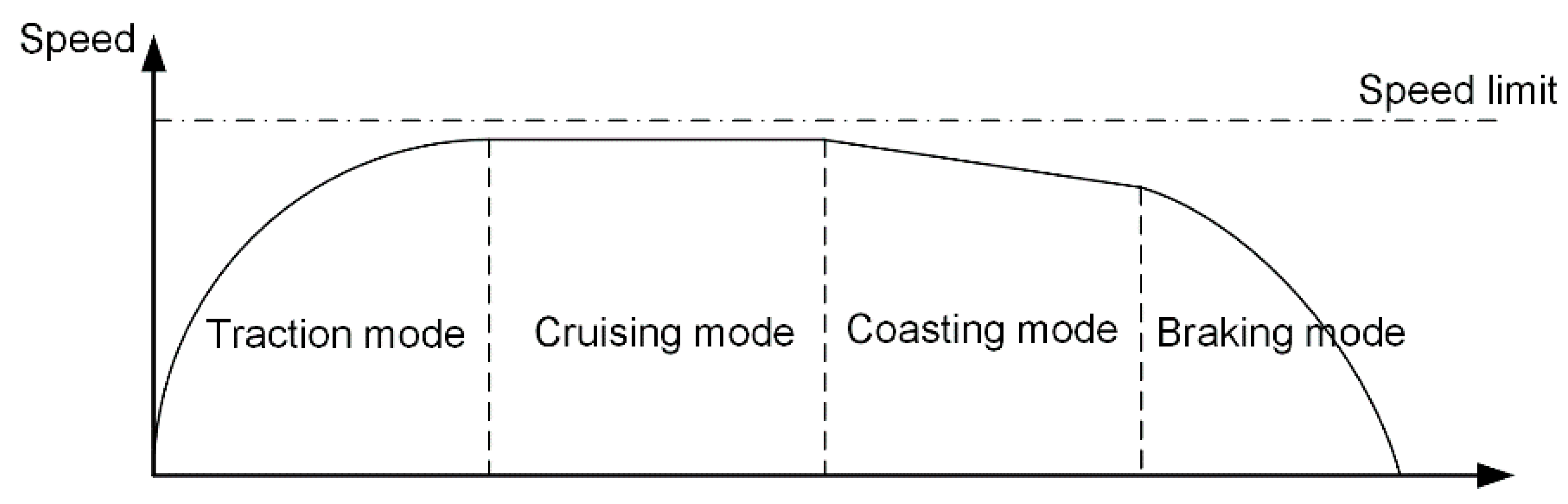
2.1.1. Train Kinematics

Train kinematics modeling can be developed using Lomonossoff’s equations as the general equations of vehicle motion. The equations are based on Newton’s second law of motion, and are subject to the train and route constraints [10,37].

$$\{\begin{array}{c}{M}_{eff}\frac{d^{2}s}{d{t}^2}=F\left(v\right)-F_{grad}-R_{cu}\left(v\right)-R_{mo}\left(v\right)\hfill \\ F_{grad}=M_{rs}gsin\left(\theta \right)\hfill \\ R_{cu}\left(v\right)=\frac{A}{RAD}{M}_{rs}g\hfill \\ R_{mo}\left(v\right)=a+b\left|v\right|+c{v}^2\hfill \end{array}$$

(1)

where s, t, and v represent the train position, time, and speed, respectively; F is the traction/braking force; R_mo is the train resistance (known as the Davis equation) with the constants a, b, and c [38]; R_cu is the curve resistance; A is a constant number, which is set at 600 in this study; RAD is the curve radius; g is the gravitational acceleration; F_grad is a component force of the weight (θ is the slope angle); and M_rs is the train mass. Typical train traction and resistance characteristics are shown in Figure 1. The data comes from rolling stock manufacturing and will be used for the case study in Section 4.

The train motion can be further described based on the time state, as shown in Equation (2):

$$\{\begin{array}{c}\dot{s}=v\hfill \\ M_{rs}\dot{v}=u_f{F}_{tr}\left(v\right)+u_b{F}_{br}\left(v\right)+R_{mo}\left(v\right)+R_{cu}\left(v\right)+F_{grad}\left(s\right)\hfill \\ F_{ad}= u{M}_{rs}g\end{array}$$

(2)

where F_tr(v) and u_f are the traction effort and the corresponding control signal, respectively; F_br(v) and u_b are the braking effort and the control signal, respectively; and F_ad is the adhesion traction, which is the friction between the steel rail and the train drive wheels. It is important to note that the train traction effort applied on the track should be smaller than the adhesion traction, otherwise the wheel will start to slip. u is the adhesion coefficient, which depends on the train speed and track environment, as shown in Figure 2.

2.1.2. Driving Controls

Based on the equation discussed in the previous section, four typical train movement modes can be produced, as shown in

Table 1. Control signals in the four movement modes.

Movement Mode	uf	ub	Equations
Traction	1	0	$M_{tr}\dot{v}=F_{tr}\left(v\right)+R_{mo}\left(v\right)+R_{cu}\left(v\right)+F_{grad}\left(s\right)$
Cruising	1	0	$M_{tr}\dot{v}=F_{tr}\left(v\right)+R_{mo}\left(v\right)+R_{cu}\left(v\right)+F_{grad}\left(s\right)=0$
Coasting	0	0	$M_{tr}\dot{v}=R_{mo}\left(v\right)+R_{cu}\left(v\right)+F_{grad}\left(s\right)$
Braking	0	1	$M_{tr}\dot{v}=F_{br}\left(v\right)+R_{mo}\left(v\right)+R_{cu}\left(v\right)+F_{grad}\left(s\right)$

and Figure 3. For example, when the train is operating in the traction mode, the signal (u_f) is 1. The traction power is then generated to increase the train speed until reaching the speed restrictions. When the train speed is small, the output traction effort is constant. After the output power reaches its maximum value, the traction effort keeps decreasing, as shown in Figure 1. However, in practice, a reduced traction effort is usually applied to the train to improve passenger comfort, especially in off-peak services. In the cruising mode, the traction power is only reduced to overcome the motion resistance, in order to keep the train running at a constant speed.

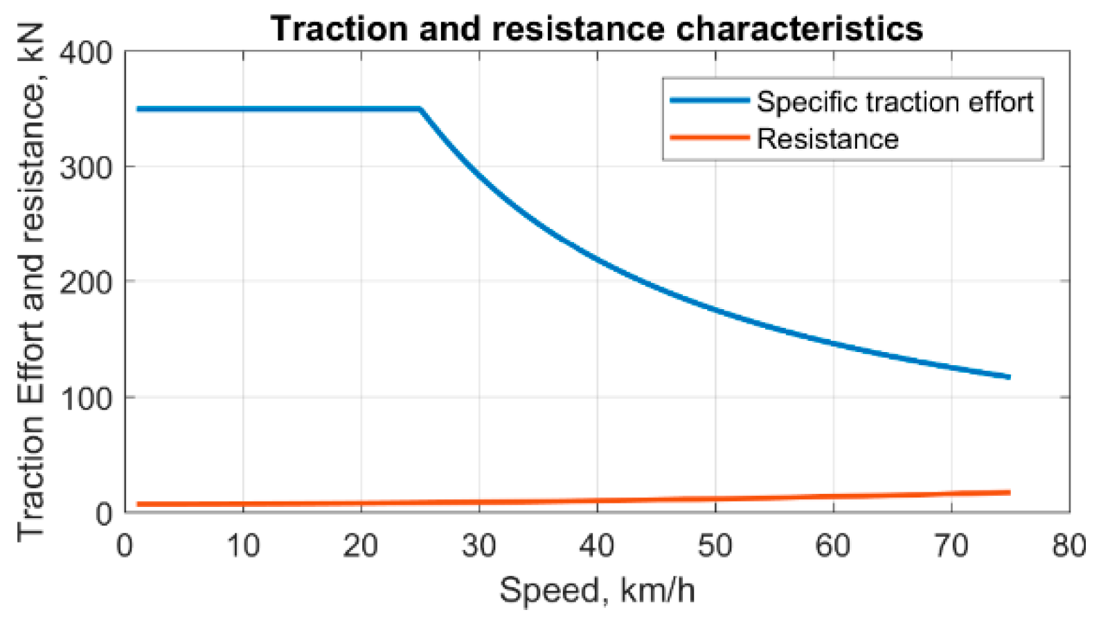
2.1.3. Train Power Demand

The train mechanical power demand can be determined by the traction controls, which can be calculated by Equation (3), where $P_{me}$ is the train mechanical power, $F_{tr}$ is the instantaneous tractive effort, and $v$ is the train speed. The electric traction power of the train ($P_{el}$) can be expressed by (4), where $\eta$ is the efficiency of power chain conversion between mechanical and electrical power (assumed as 85% in this paper). The mechanical power is positive when the train is in traction mode, while it is negative when the train is braking.

$$P_{me}=F_{tr}\times v$$

(3)

$$P_{el}=\{\begin{array}{cc}\frac{P_{me}}{\eta }& if P_{me}\ge 0\\ P_{me}\times \eta & if P_{me}<0\end{array}$$

(4)

Besides the electric traction power demand, the air conditioning and lighting on the train require electric auxiliary power. The auxiliary power can be high in the summer or winter due to a higher demand for cooling or heating devices, respectively. The total train power demand ($P_{train\_demand}$) can be calculated by summing the electric traction power demand and auxiliary power ($P_{aux}$) using Equation (5). The train power demand is a dynamic value in the time domain, which is an input of the model of the traction power network.

$$P_{train\_demand}=P_{el}+P_{aux}$$

(5)

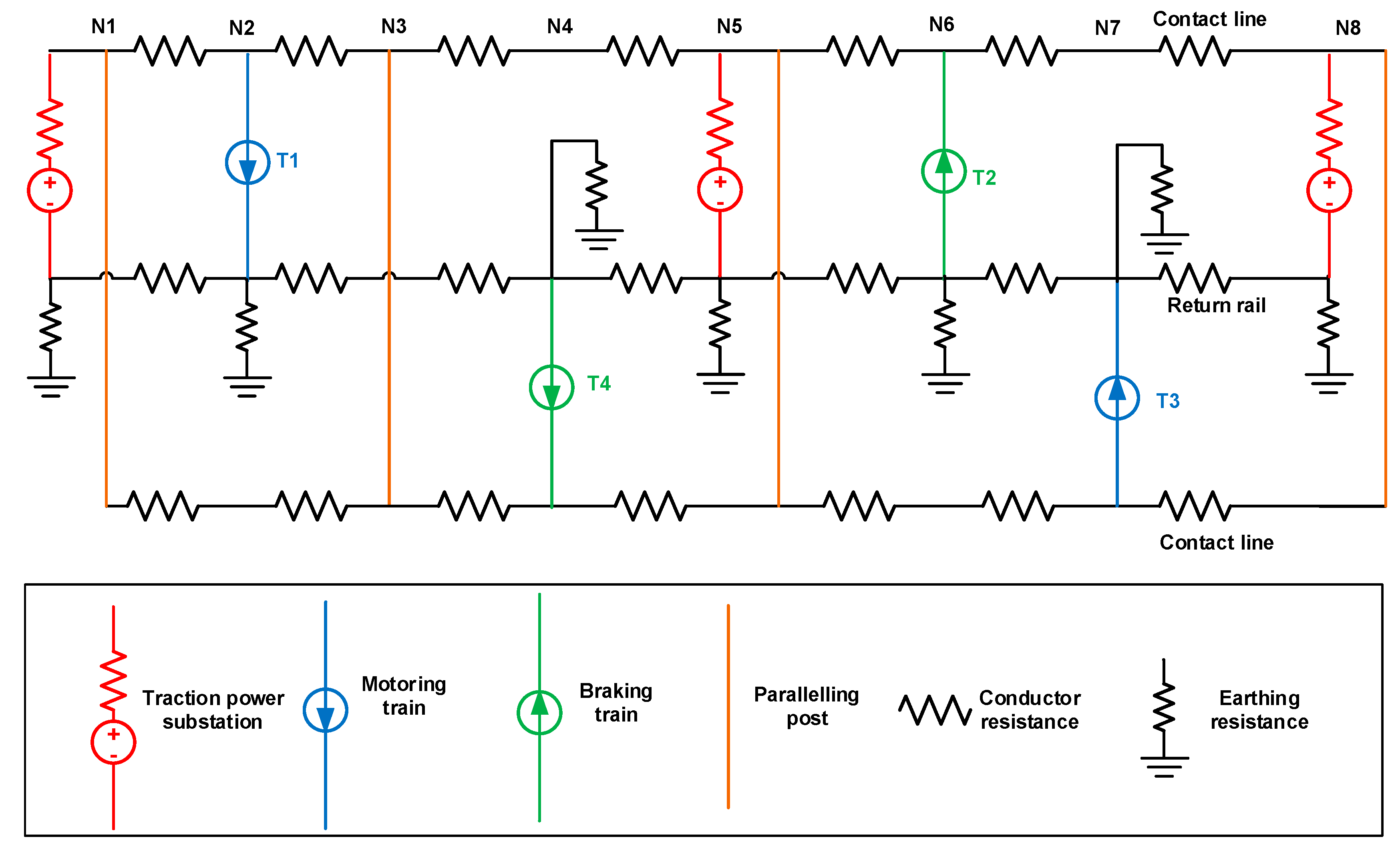
2.2. Traction Power Network Modeling

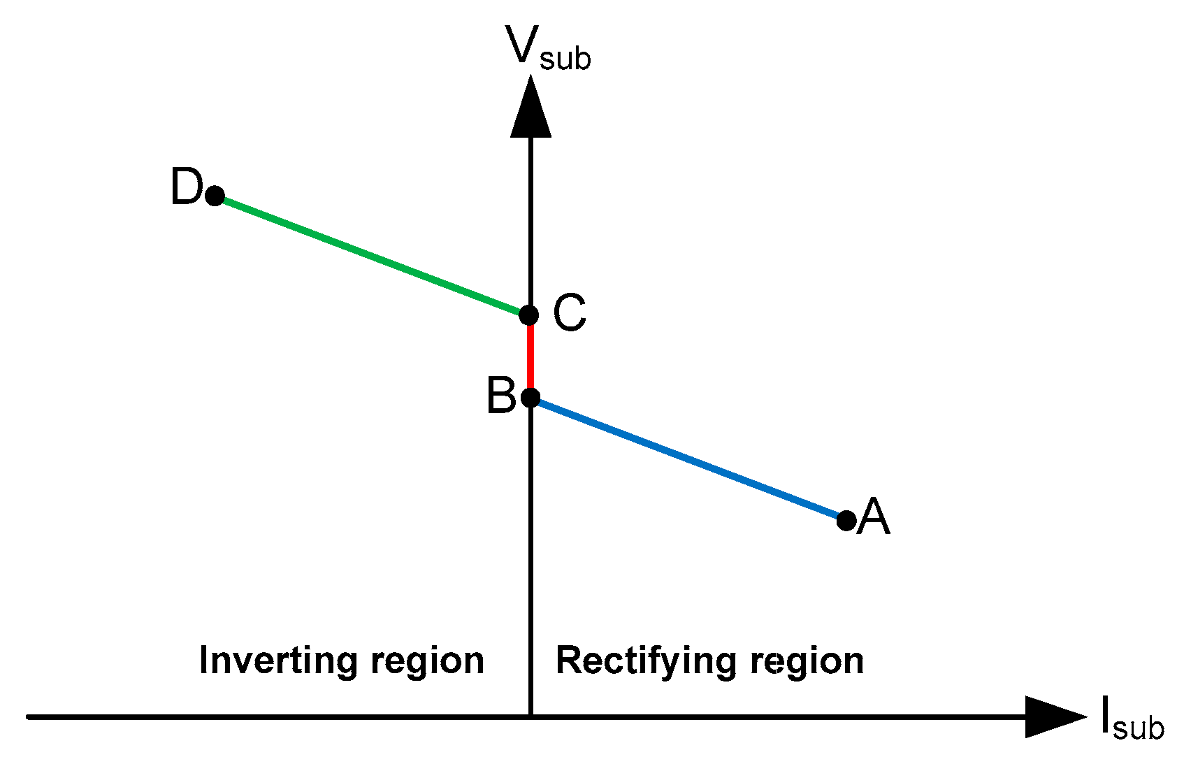
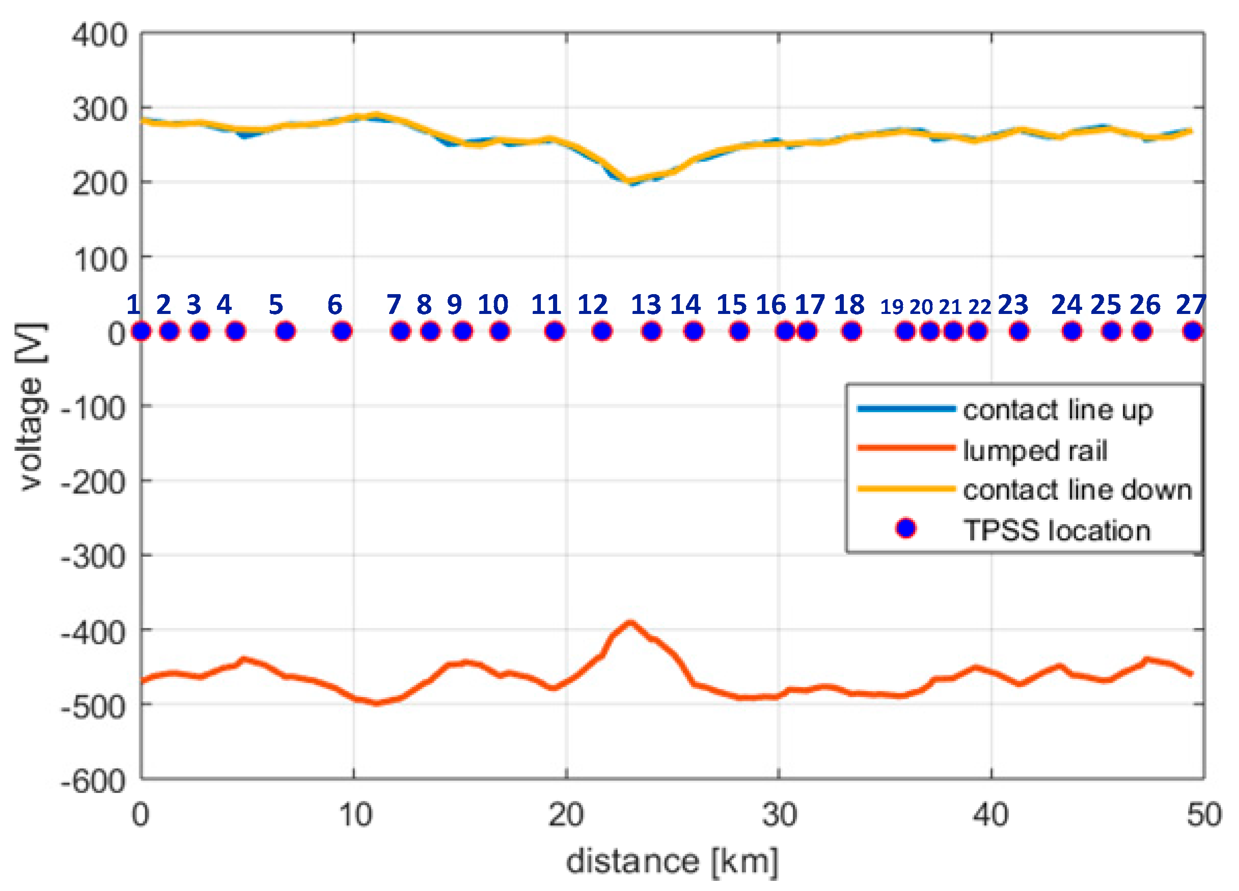
2.2.1. Traction Power Substation

In the DC railway traction power supply network, a traction power substation (TPSS) is used to power trains. Some modern DC railway systems implement both rectifiers and inverters in the TPSS. The rectifier converts AC power to DC power to supply trains requiring traction power, while the inverter converts DC power to AC power and transmits regenerative braking power from trains back to the AC network.

The rectifier output voltage normally decreases when the load power or load current vary [39]. In this simulation, the output voltage characteristic of the TPSS is simplified by a piecewise function, as shown in Figure 4. The rectifier output voltage curve shown as ‘A-B’ can be calculated using Equation (6). $r_{rec}$ is a virtual resistance, which represents the decreasing characteristics of the rectifier voltage, but does not dissipate any resistive power losses. The value of $r_{rec}$ is derminated by the rated power and current of the rectifier. The inverter used in a railway substation can be based on a thyristor or IGBT, where the output voltage can be fully controlled to follow a fixed slope like ‘C-D’ in Figure 4. The inverter output voltage can be derived using Equation (7), where $r_{inv}$ represents the slope rate, but does not dissipate power losses. $r_{inv}$ can be modified by the control strategies of the inverter to meet the requirement of power receptivity. The trigger voltage of the inverter is shown at point ‘C’, which is normally higher than the no-load voltage of the rectifier at point ‘B’ to avoid current circulation between the rectifier and inverter.

$$V_{rec}=V_{noload}-r_{rec}\times I_{rec}$$

(6)

$$V_{inv}=V_{trigger}-r_{inv}\times I_{inv}$$

(7)

2.2.2. Power Network Circuit

The traction power network consists of substations, the contact line, return rails, and multiple trains. Figure 5 illustrates an equivalent circuit of a railway traction power network. A paralleling post is represented by a conductor connecting the contact lines on the up and down tracks. The paralleling post can improve the line voltage and reduce transmission power losses. The contact lines are modeled by conductor resistors split by trains, substations, and parallel posts. The return rails on both tracks can be lumped for simplification, which reduces the computing time with a reasonably low error [40]. The resistance of the contact line and lumped rail is determined by the length and resistivity of the conductor given by (8), where ${\rho }_c$ and ${\rho }_r$ are the resistivity of the contact line and return rail per track, respectively. The resistance is split by trains and substations. When trains move, the resistance of the network will be changed according to the location of trains. Based on train motion modeling, the location of trains can be obtained and the length of resistance between trains and substations can be calculated. The earthing resistance is connected with every substation and train.

$$\{\begin{array}{c}{R}_c=L\times {\rho }_c\\ R_r=L\times \frac{{\rho }_r}{2}\end{array}$$

(8)

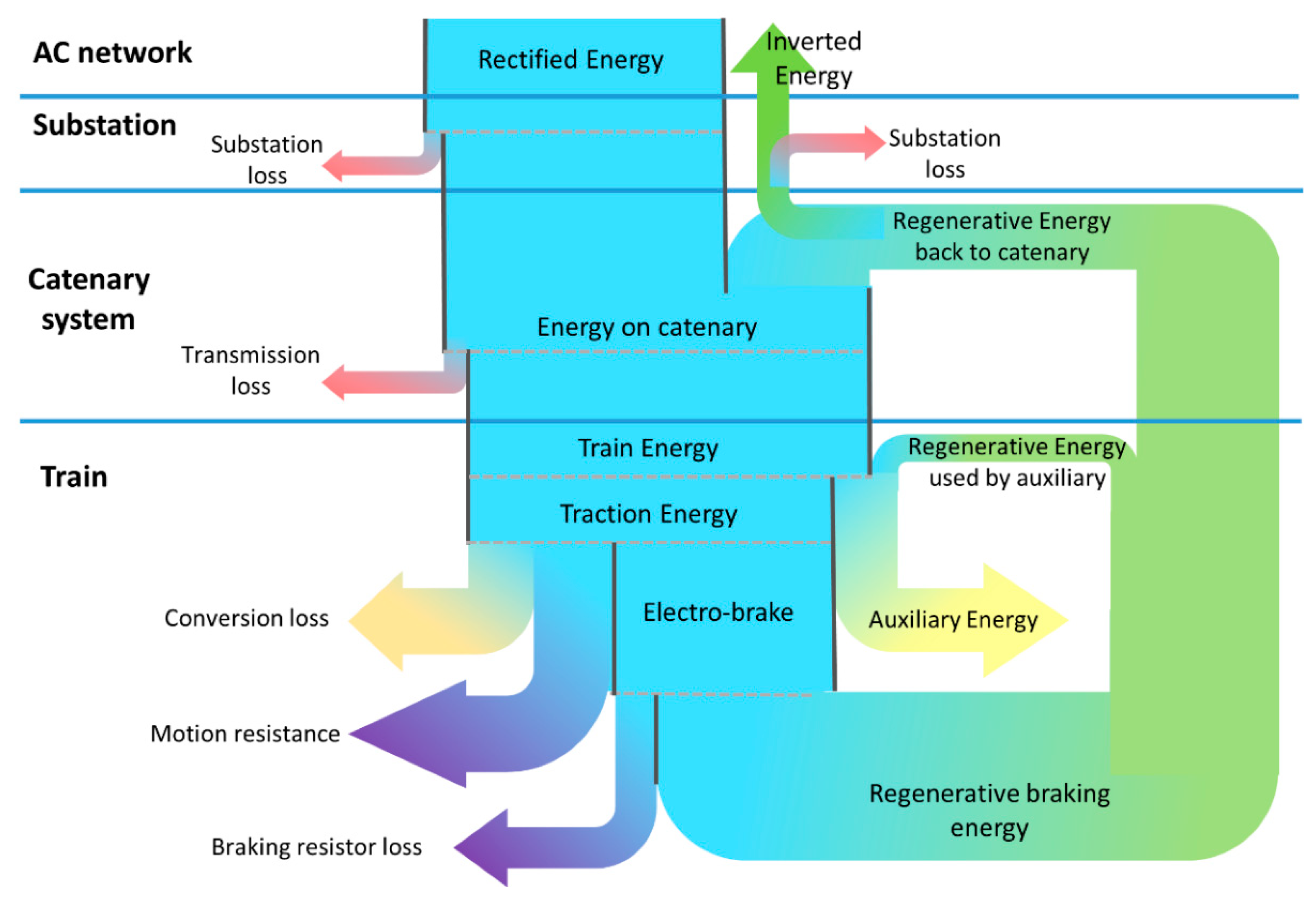
2.3. Energy Flow and Evaluation

By integrating the train and traction power network modeling, the energy flow through the whole network can be evaluated and analyzed. The energy flow of railway systems can be divided into four levels, as shown in Figure 6.

The railway energy is fed from the AC electricity grid. The traction substation energy is rectified from the AC network and the surplus regenerative braking energy can be inverted back to the AC network. Therefore, the global system energy consumption ($E_s$) can be calculated using Equation (9), where $E_{rec}$ is the energy from the rectifier and $E_{inv}$ is the energy from the inverter.

$$E_s=E_{rec}-E_{inv}$$

(9)

Electricity through rectifiers and inverters can generate substation losses ($E_{sl}$). The rectifier power efficiency (${\eta }_{rec}$) and inverter power efficiency (${\eta }_{inv}$) are assumed to be constants in this paper, with values of 97% and 95%, respectively. Therefore, the substation losses can be calculated using Equation (10).

$$E_{sl}=E_{rec}\times (1-{\eta }_{rec})+E_{inv}\times \left(1-{\eta }_{inv}\right)$$

(10)

The electricity from substations is transmitted to the DC catenary system to supply moving trains. The current through conductor rails generates transmission loss ($E_{tl}$), which is determined by the resistance of the conductor rail ($r_{conductor}$) and the current passing through it using Equation (11).

$$E_{tl}=\int r_{conductor}\times i^{2}dt$$

(11)

The train energy ($E_{tr}$) from the DC catenary system is used for the traction and auxilary system. Part of the traction energy is dissipated by onboard converters and motion resistance. The train obtains kinetic energy, which is finally dissipated by braking systems. The train energy can be expressed in (12), where $E_{cl}$ is the conversion loss, $E_{mr}$ is the energy required to overcome motion resistance, $E_{eb}$ is energy for the electro-braking system, and $E_{aux}$ is energy for the auxilary system.

$$E_{tr}=E_{cl}+E_{mr}+E_{eb}+E_{aux}$$

(12)

Part of the energy for the electro-braking system can be regenerated and reused by the auxiliary system directly or transmitted back to the catenary system. However, too much regenerative power can increase the train voltage. To protect the train from overvoltage, the surplus electro-braking energy is dissipated by the braking rheostat. To evaluate the efficiency of regenerative braking energy, the regeneration efficiency (${\eta }_{reg}$) is defined using Equation (13), where $E_{reg}$ is the useable regenartive braking energy and $E_{eb\_r}$ is the energy dissipated by the braking rheostat.

$${\eta }_{reg}=\frac{E_{reg}}{E_{eb}}=\frac{E_{reg}}{E_{eb\_r}+E_{reg}}$$

(13)

From the railway system level, the energy flow should be consistent with the energy conservation equation shown in (14), where the global system energy consumption is equal to the sum of substation loss, transmission loss, and train energy deduced by the regenerative braking energy. The system energy flows have complicated relationships with each other. A comprehensive evaluation of the infrastructure parameters and operation controls is normally required to identify the energy flow characteristics of a practical railway line.

$$E_{rec}-E_{inv}=E_{sl}+E_{tl}+E_{tr}-E_{reg}$$

(14)

3. Fault Identification

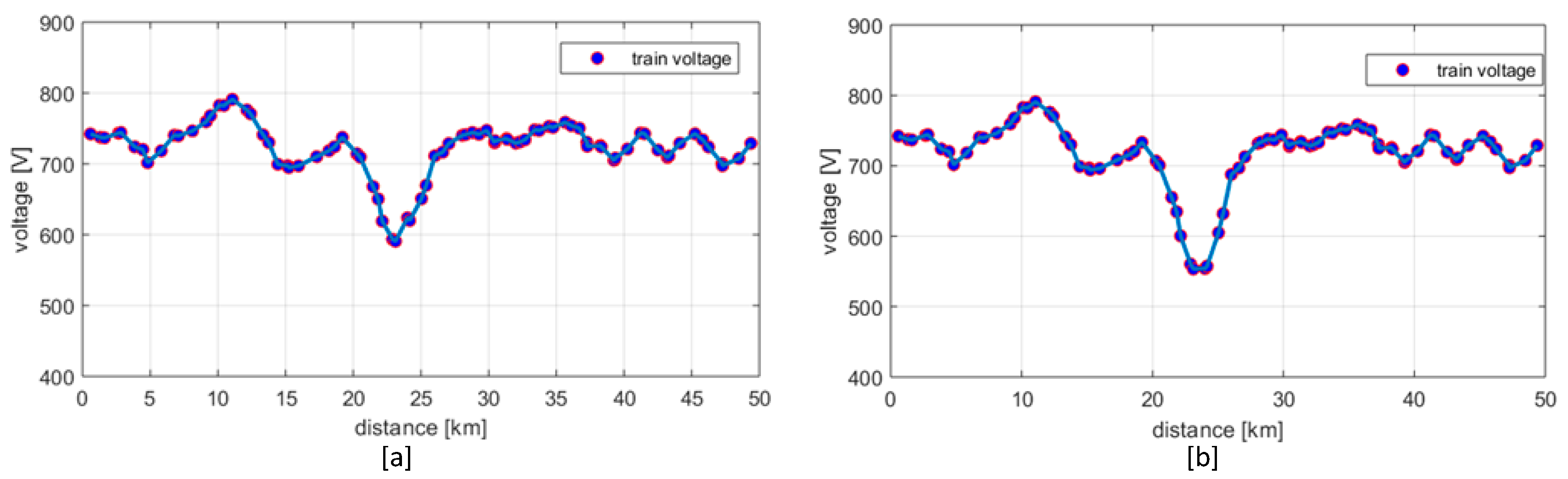
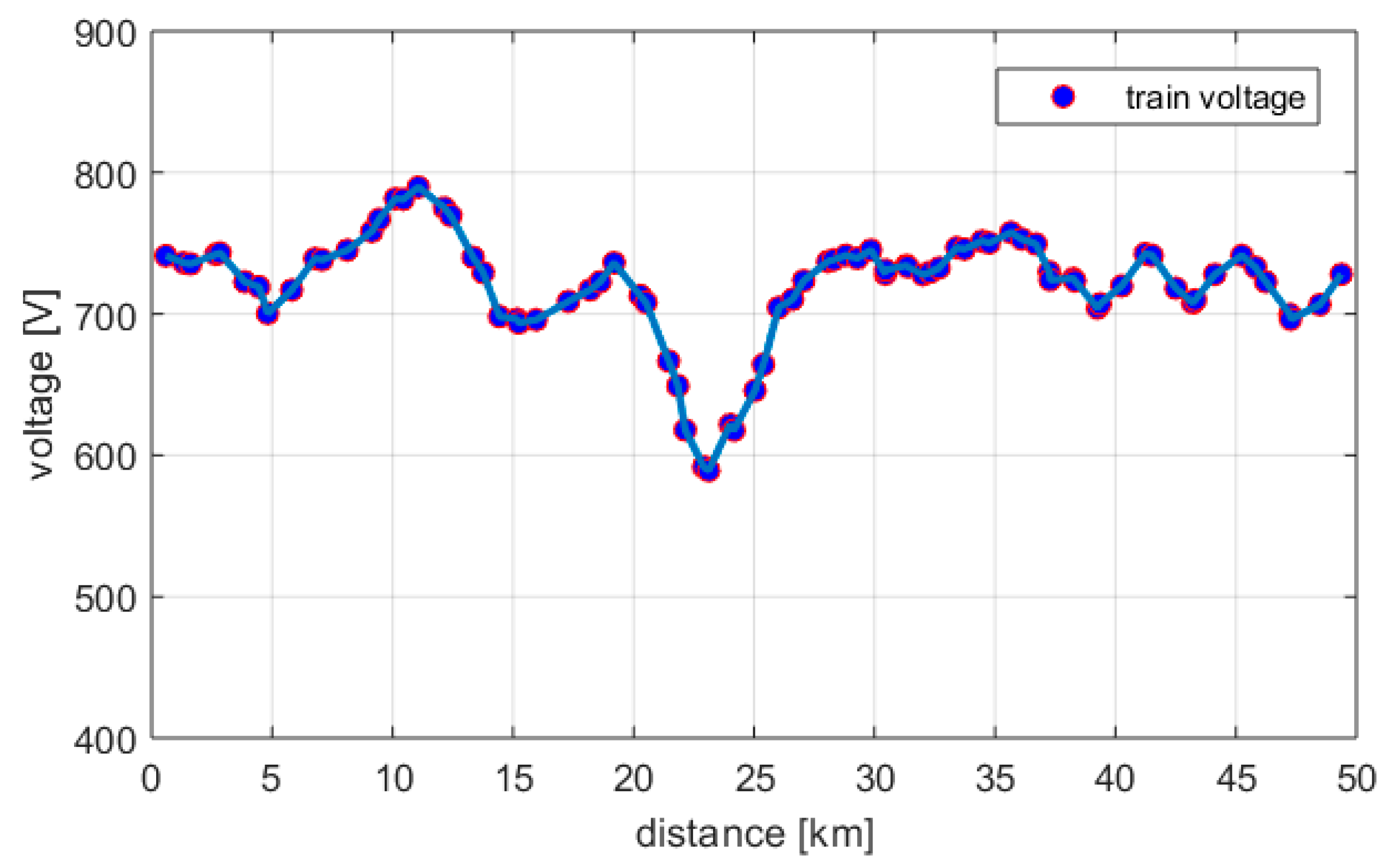
3.1. Under-Voltage Traction

When the train power demand is known, the electric circuit of the traction power network can be solved using power flow analysis algorithms. The train voltage and current can be obtained, which is consistent with Equation (15).

$$P_{train}=I_{train}\times V_{train}$$

(15)

Trains normally collect enough power from the traction power network to meet the traction demands. However, sometimes, the traction power demand might not be fully supplied due to the low network voltage when the traction power network is weak. In order to protect the train traction devices and power networks, the control devices on-board will adapt the train power demand. To study the train and network load performance, a comprehensive representation of the train model is required.

The British Standard in Railway Applications-Power Supply and Rolling Stock introduces the maximum allowable train current against the train voltage, as shown in Figure 7 [41]. The train traction modes can be categorized into three regions according to the pantograph voltage levels. In region 1, the train voltage is lower than the lowest non-permanent voltage Vmin. The train only receives the energy to supply the auxiliary system, and not the train traction system. In region 2, the train voltage is between Vmin and aVn, where $V_n$ is the nominal voltage of the system and $a$ is the knee point factor, which is lower than 1 (normally between 0.8 and 0.9). In this region, the under-voltage traction mode is activated. The train traction current is limited, which means that the train cannot receive the maximum traction power. In region 3, the train voltage is higher than Vn, where the train is in the normal traction mode. The maximum traction power of the train can be fully supplied from the power network. Taken from the British Standard in Railway Applications-Supply Voltages of Traction Systems [42], the voltage characteristics, including under-voltage and over-voltage levels for DC railway systems, are specified in

Table 2. Permissible voltage limits for DC railways [42].

DC Railway Voltage Level (V)	Lowest Non-Permanent Voltage Vmin (V)	Rated Voltage Vn (V)	Highest Non-Permanent Voltage Vmax (V)
600	400	600	800
750	500	750	1000
1500	1000	1500	1950

. In this paper, the under-voltage traction mode is considered in the substation load analysis to evaluate the traction power supply capability.

3.2. Rail Potential

For DC railway power systems, trains collect current from the overhead line or third rail and then return the current by the running rails. The return current will increase the rail potential, which is determined by the train traction power and location. To understand the rail potential, the earthing resistance is considered in the simulation. The earthing leakage resistance coefficient ($C_e$) for the railway network is around 10 Ω·km. For the lumped rail network in Figure 5, the earthing resistance is calculated by (16).

$$R_e=\frac{2\times C_e}{L}$$

(16)

3.3. TPSS Outage

A traction power substation (TPSS) can be switched off when there is a fault current or during maintenance. The railway traction power network should supply enough power to trains when one of the substations is switched off. To switch off one substation in the simulation, the rectifier resistance ($r_{rec}$) in (6) is set to a large value, which is 1 MΩ in this paper. Therefore, the output current from the rectifier substation is limited to zero.

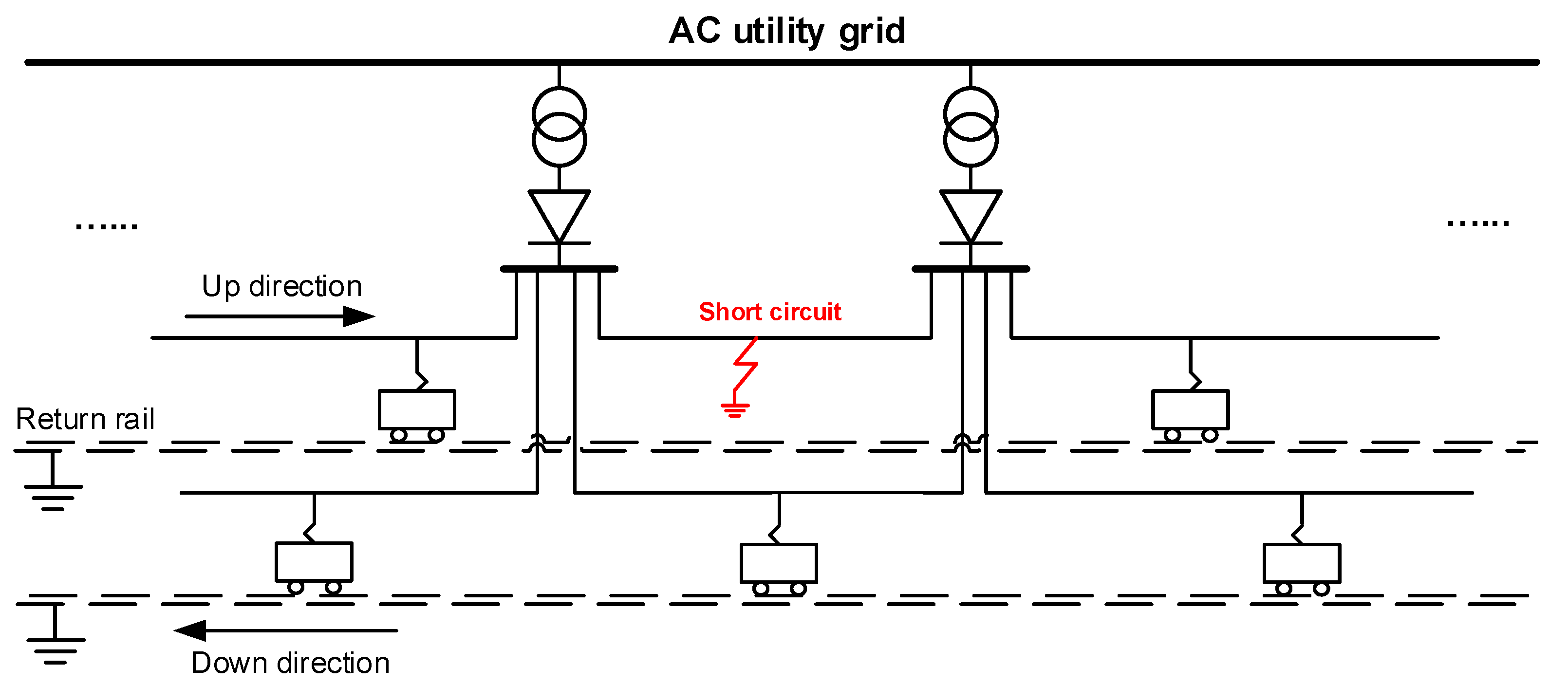
3.4. Short Circuit

A short-circuit fault has a significant impact on the rail power network. Figure 8 presents the topology of a short-circuit fault, which connects the contact line with the earth. To study the impact of a short-circuit fault, a small resistance is inserted into the network circuit in Figure 5. The value of the short-circuit resistance will also affect the performance of the traction power supply.

4. Case Studies

4.1. Simulation Parameters

A mathematical simulation was developed in a MATLAB script based on the methods illustrated in the previous section. In order to evaluate and identify the developed method, a case study was carried out based on a metro line in Singapore. The line is 51 km long, with 32 passenger stations and 27 substations. In total, 26 of all substations are implemented with rectifiers for the traction power supply and 10 of them are implemented with inverters. TPSS-2 is only implemented with an inverter without a traction power supply. The rated power for the traction substation is 4 MW, except for TPSS-6, which has been upgraded to 6 MW. The dwell time and terminal time are 40 and 200 s, respectively. The rolling stock uses a DC 750 V third rail power supply system with a regenerative braking system. The train characteristics are shown in

Table 3. Train characteristics.

Parameters	Value/Equation
Train mass with passengers, tonnes	301
Train formation	3M3T
Train length, m	148
Rotary allowance	0.08
Train Resistance, N/tonne	3.49 + 0.039 v + 0.00066 v2 (v: km/h)
Maximum traction and braking power, kW	2518
Maximum operation speed, km/h	80
Maximum traction effort, kN	351

.

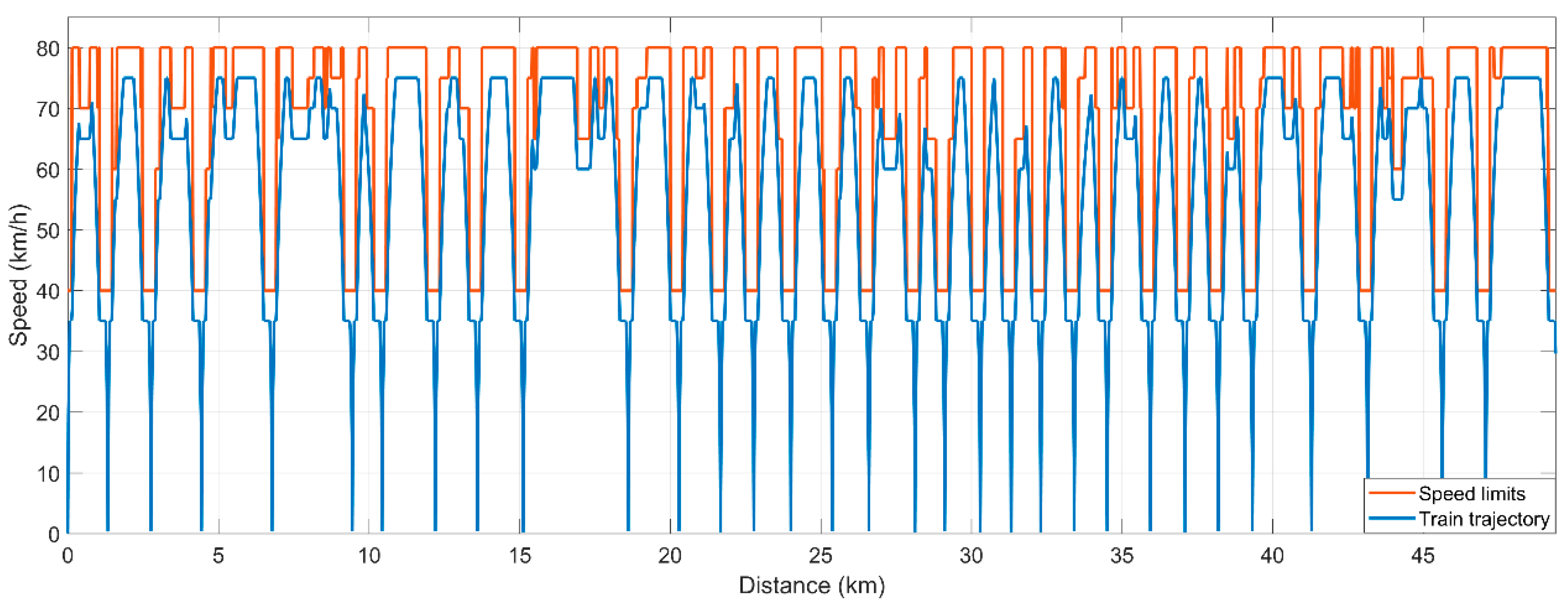
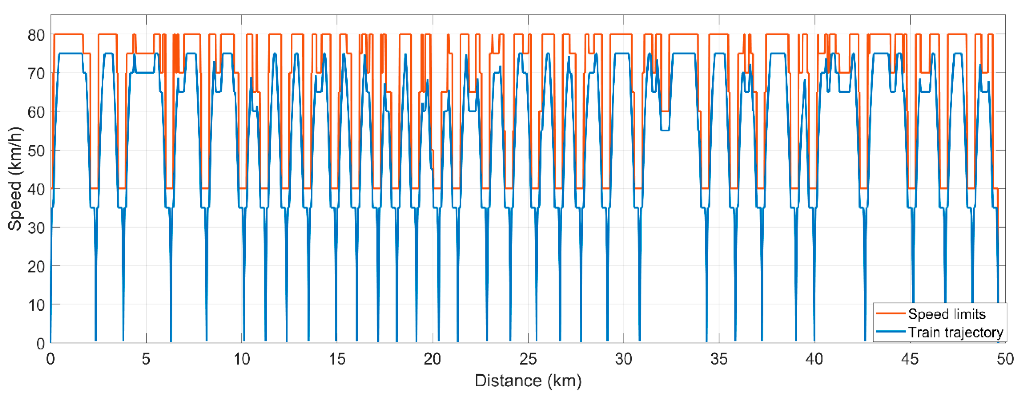
4.2. Train Motion Simulation Results

Based on the train traction characteristics and line data shown above, the train motion simulation results are presented in Figure 9 and Figure 10. The single journey times for the up-direction operation and down-direction operation are 4917 and 4958 s, respectively. It can be observed that the train does not apply the coasting mode throughout the journey, in order to achieve a smaller journey time and greater line capacity. Furthermore, the train maximum operation speeds are always 5 km/h slower than the line speed restrictions, in order to reduce the possibility of activating the automatic train protection (ATP) system by mistake.

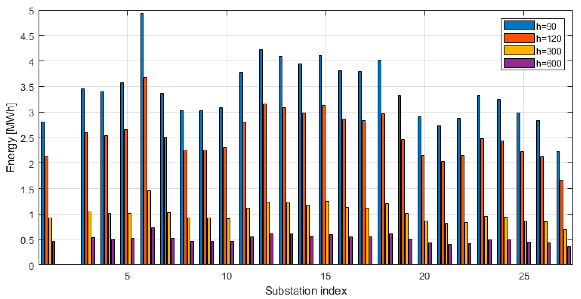
4.3. Energy Consumption with a Normal Operation

The simulation results of energy consumption will be analyzed in this section. In this case study, the speed restriction along stations was 40 km/h. Since the multi-train operation was repeated every headway period, the energy consumption during the headway period was compared, as shown in

Table 4. Energy consumption of the 40 km/h case study.

Scenario Index	1	2	3	4	5	6	7	8	9	10
Auxiliary Power (kW)	0	0	0	0	0	480	480	480	480	480
Headway (s)	90	100	120	300	600	90	100	120	300	600
Es (kWh)	802	796	825	840	845	2221	2221	2214	2199	2191
Erec (kWh)	816	803	859	957	1066	2221	2221	2215	2209	2224
Einv (kWh)	−14	−8	−34	−117	−222	0	0	0	−10	−34
Esl (kWh)	25	24	28	35	44	67	67	66	67	69
Efl (kWh)	16	13	17	12	10	84	73	67	33	21
Etl (kWh)	48	46	65	74	74	74	72	81	72	74
Etr_demand (kWh)	1507	1507	1507	1507	1507	1507	1507	1507	1507	1507
Etr (kWh)	1507	1507	1506	1507	1507	1476	1489	1479	1507	1507
Eeb (kWh)	796	796	796	796	796	796	796	796	796	796
Ereg (kWh)	794	795	791	788	790	796	796	796	796	796
Eaux (kWh)	0	0	0	0	0	1316	1316	1316	1316	1316
ηreg	100%	100%	99%	99%	99%	100%	100%	100%	100%	100%
Time of under-voltage (s)	0	0	8	0	0	312	192	250	3	0
Time of train running (s)	9900	9900	9900	9900	9900	9900	9900	9900	9900	9900

. The results show a comparison of 10 scenarios with different auxiliary powers (0 or 480 kW) and headways (90, 100, 120, 300, and 600 s). The energy consumption results denote the following:

• When the auxiliary power is 0 kW, there is some energy inverted by substations. The inverted energy increases when the headway increases. When the headway is short, most regenerative braking energy is used by motoring trains in DC systems;
• When the auxiliary power is 480 kW, not much energy is inverted by substations. The inverted energy when the headway is 90, 100, and 120 s is zero, and the inverted energy increases a little when the headway is 300 and 600 s. This is because the train auxiliary uses a lot of regenerative braking energy;
• The time interval is 1 s in the simulation. When the headway is 90 s, there are 110 trains in the network. Therefore, there are 9900 train seconds in the simulation of each scenario. The time of under-voltage means the amount of time when the under-voltage traction mode occurs. When the auxiliary power is zero, the time of under-voltage is very low. However, when the auxiliary power is 480 kW, under-voltage happens 312 times during the operation. The time of under-voltage decreases when the headway increases;
• The regenerative energy efficiency is very high for all of the scenarios, and is between 99% and 100%. This denotes that nearly all of the electro-braking energy can be reused;
• The total system loss is the sum of the substation, feeder, and transmission loss. The loss accounts for around 10% of the total substation energy consumption.

The energy consumption for the one-hour operation was calculated by a simulation. Four cases with different headway times (90, 120, 300, and 600 s) were compared and the results are shown in Figure 11. The energy consumption of each TPSS during the 1 h operation results denote the following:

• The total energy consumption of all TPSS decreases with the headway time;
• The maximum energy consumption occurs at TPSS-6 for the cases which are shown in red. This denotes that TPSS-6 could consume more energy than others for most cases. This is consistent with the fact that the rated tractive power of TPSS-6 is 3 MW × 2, which is higher than other the TPSS;
• The second highest energy consumption occurs at TPSS-12 for the cases;
• The energy consumption of each TPSS varies with different timetables. Some TPSS could consume a high amount of energy due to a particular timetable.

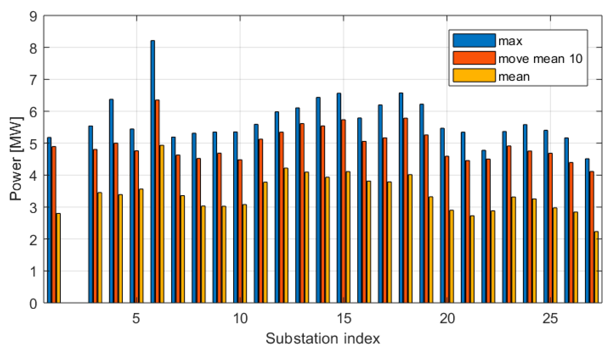
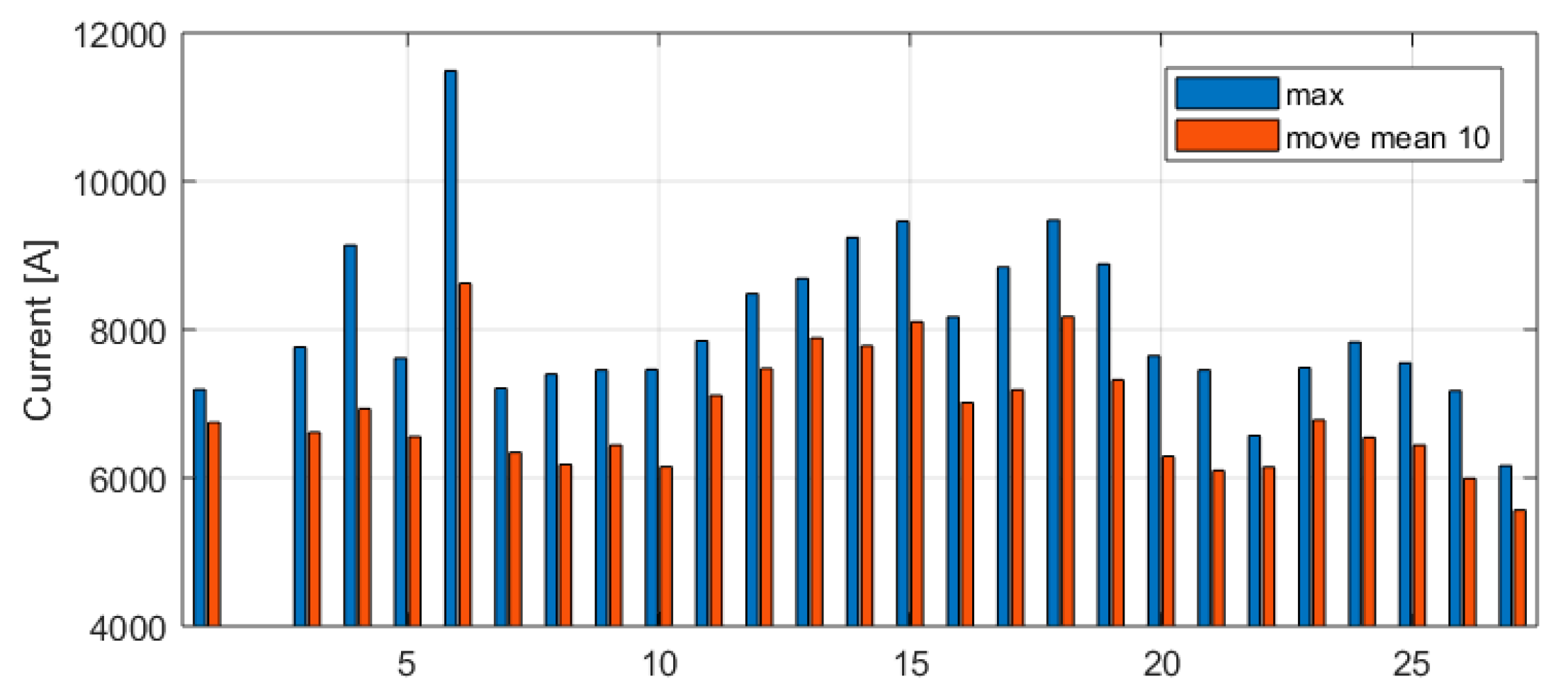
4.4. Study of Hotspots

With the increase of train services, the TPSS power demand will increase, which might cause tripping at hotspot stations. In this case study, TPSS-2 is a tie station without a traction power supply. The following study of the hotspot is based on the operation with the headway of 90 s. The substation traction power, output current, and touch potential are used to analyze the hotspot stations.

Figure 12 shows the maximum traction power, the maximum moving mean traction power over 10 sections, and the average traction power of each substation during the operation. It can be seen that TPSS-4, TPSS-6, TPSS-14, TPSS-15, and TPSS-18 output the highest peak power and average power. The hotspot stations are around the area of TPSS-4, TPSS-5, and TPSS-6, and the area of TPSS-14, TPSS-15, TPSS-17, and TPSS-18, which require careful monitoring to avoid overload faults.

The current and voltage of each substation are compared in Figure 13 and Figure 14. The current of hotspot stations is usually high, and the voltage of hotspot stations is usually low. The reason for the hotspots is mainly because of the design and location of substations. In addition, the train operation has an impact on the hotspots. Therefore, it is necessary to avoid heavy acceleration in the hotspot areas.

4.5. Results with TPSS Switched off

4.5.1. Network Operation Results

In this scenario, the headway was set to 120 s and 82 trains were running on the network. In a normal operation, TPSS-13 supplies the highest traction power, with 6490 kW. The railway power network was studied when TPSS-13 was switched off. The network working status before and after switching off TPSS-13 is compared in

Table 5. Traction power substation (TPSS) result comparison.

	TPSS Index	Positive Feeder Potential (V)	Negative Feeder Potential (V)	Output Voltage (V)	Current (A)	Power (kW)
Normal operation	10	722	3	720	3622	2760
	11	728	−9	737	2600	2012
	12	704	39	665	6909	4999
	13	690	66	624	9333	6490
	14	719	9	711	4159	3143
	15	730	−12	742	2270	1765
	16	728	−9	738	2527	1957
TPSS-13 switched off	10	718	0	718	3701	2887
	11	723	−9	732	2864	2234
	12	696	45	651	7716	6019
	13	663	109	554	0	0
	14	708	21	687	5596	4365
	15	724	−11	734	2747	2143
	16	724	−11	735	2671	2083

and Figure 15. It can be seen that the output voltage at TPSS-13 decreases from 690 to 663 V, and the contact line potential decreases around TPSS-13. However, the potential at the TPSS-13 negative feeder increases from 66 to 109 V, and the rail potential increases to over 100 V around TPSS-13. Due to the outage of TPSS-13, the nearby TPSS supply a higher tractive power. The output current of TPSS-12 increases from 6909 to 7716 A, while the output power increases from 4999 to 6019 kW. The output current of the TPSS-14 increases from 4159 to 5596 A, while the output power increases from 3143 to 4365 kW. The train voltage results are compared in Figure 16. Due to one of the TPSS being switched off, the train voltage around TPSS-13 decreased, leading to five trains being in under-voltage mode.

4.5.2. Energy Consumption

The impact of TPSS outage on the network energy consumption is evaluated in this section. The scenarios when one TPSS is switched off were simulated for a one-hour operation. The headway time was 120 s. Figure 17 compares the energy consumption of six substations with various outage modes, including a no outage mode and one of the first nine TPSS outages. When the TPSS is switched off, the energy consumption for that TPSS is zero. The results denote that the network is capable of supplying enough tractive power to the trains when one of the TPSS is switched off. The following comments can be made by comparing the energy consumption when one TPSS is switched off:

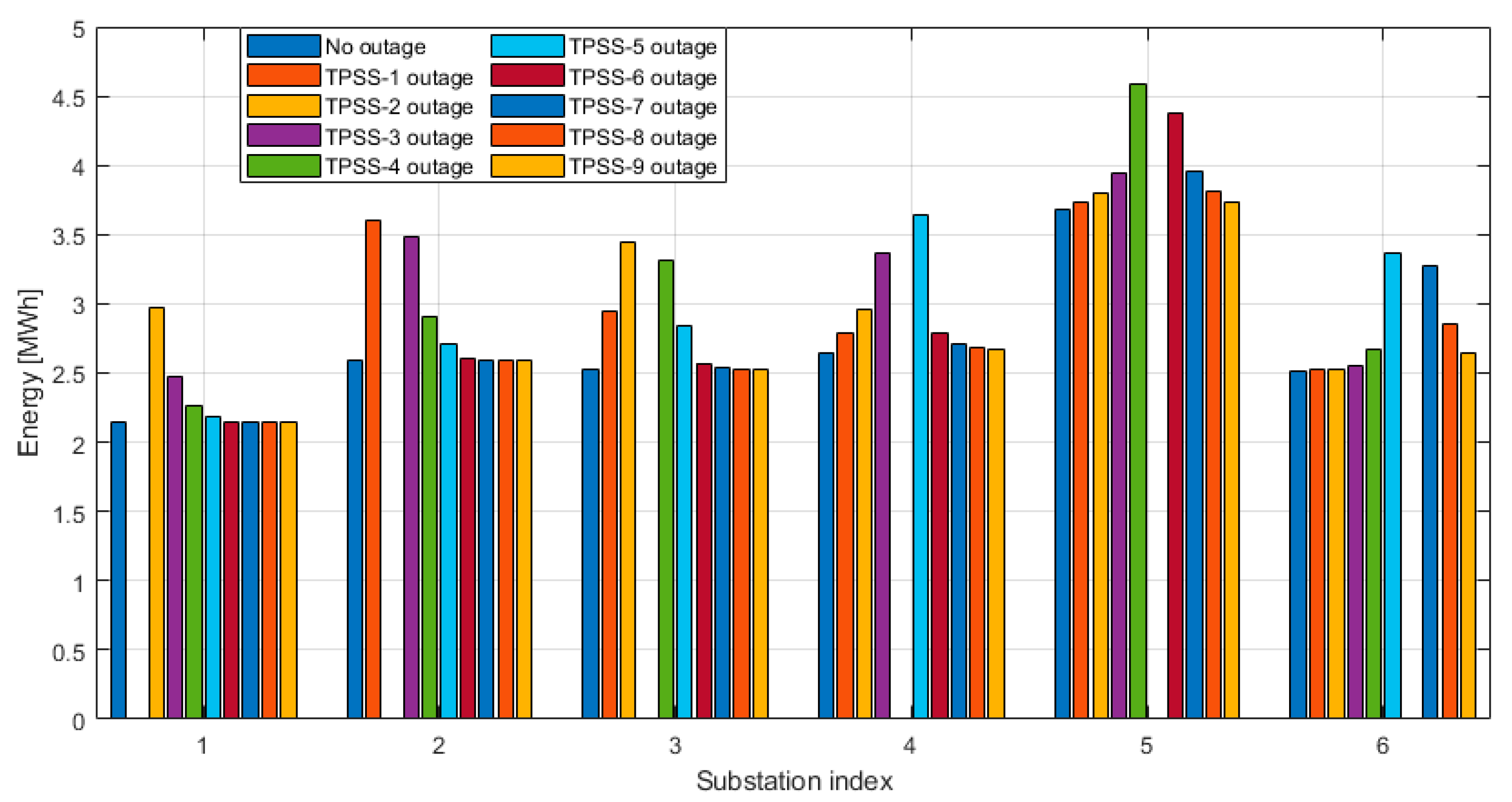
• If one of the TPSS is switched off, the energy consumption of this TPSS is zero. The energy consumption of TPSS around this faulty TPSS increases;
• The amount of energy consumption change of the working TPSS depends on the distance from the outage TPSS. The maximum variation occurs on the nearest working TPSS, which can represent up to 39% of the increase;
• The substation energy consumption is unlikely to be affected if there are more than three substations between this substation and the outage substation;
• If the fault TPSS supplied a very large amount of energy when it was on, the impact on the nearby TPSS will be more significant when this faulty TPSS is down.

4.6. Results with a Short Circuit

In this section, the simulation results are studied when a short-circuit fault occurs at 26 km between TPSS-14 and TPSS-15. The short circuit resistance is 0.1 Ω, which short connects the contact line up and the earth. Figure 18 shows the network voltage when a short circuit occurs. The potential of the contact line and the rail potential decrease a lot. Figure 19 shows the train voltage when a short circuit occurs. The train voltage is not particularly affected. Because the absolute rail potential becomes very high, the whole network will be switched off for protection.

5. Conclusions

A holistic modeling method for evaluating the power supply capability for DC railway traction power systems has been illustrated in this paper. The mathematic simulation integrates the train kinematics, driving controls, power supply infrastructure, and multiple fault modes. A case study based on a metro line in Singapore has been developed to compare the load performance with various train operation strategies and fault modes. The results denote that under-voltage traction is activated by reducing the headway time. By evaluating the instantaneous power supply and energy consumption of substations, the hotspot area can be identified. By understanding the hotspot stations, train operators can improve the power network reliability by reducing the acceleration rate or upgrading the traction power substation capacity. The case study also illustrates the load performance when some substations are switched off due to a fault current or maintenance. The substation outage could increase the rail potential and reduce the train voltage. Therefore, it is necessary to understand the impact of substation outage before conducting maintenance. The results also indicate that the outage of a substation can increase the energy demand of nearby substations by up to 39%. The impact on the substation power load reduces with the distance from the outage substation. The substation power load is rarely increased when the outage occurs at more than three substations away from it. The short-circuit faults can affect the rail potential significantly, which will trip the network for protection.

Based on the simulation and evaluation, the reliability of the traction power network can be analyzed and predicted, which can be studied in the future. The health and usable life of the power support equipment can be evaluated and optimized by improving the train operation and infrastructure design.

References

- Chymera, M.Z.; Renfrew, A.C.; Barnes, M.; Holden, J. Modeling Electrified Transit Systems. IEEE Trans. Veh. Technol. 2010, 59, 2748–2756. [Google Scholar] [CrossRef]
- Chang, C.S.; Khambadkone, A.; Zhao, X. Modeling and simulation of DC transit system with VSI-fed induction motor driven train using PSB/MATLAB. In Proceedings of the 4th IEEE International Conference on Power Electronics and Drive Systems, Denpasar, Indonesia, 25 October 2001; Volume 2, pp. 881–885. [Google Scholar]
- Goodman, C.J.; Sin, L.K. DC railway power network solutions by diakoptics. In Proceedings of the IEEE/ASME Joint Railroad Conference, Chicago, IL, USA, 22–24 March 1994; pp. 103–110. [Google Scholar]
- Goodman, C.J. Modelling and simulation. In Proceedings of the 5th IET Professional Development Course on Railway Electrification Infrastructure and Systems (REIS 2011), London, UK, 6–9 June 2011; pp. 22–31. [Google Scholar]
- Cai, Y.; Irving, M.; Case, S. Modelling and numerical solution of multibranched DC rail traction power systems. IEE Proc. Electr. Power Appl. 1995, 142, 323. [Google Scholar] [CrossRef]
- Arboleya, P.; Mohamed, B.; El-Sayed, I. DC Railway Simulation Including Controllable Power Electronic and Energy Storage Devices. IEEE Trans. Power Syst. 2018, 33, 5319–5329. [Google Scholar] [CrossRef]
- Zhang, J.; Wu, M.; Liu, Q. A Novel Power Flow Algorithm for Traction Power Supply Systems Based on the Thévenin Equivalent. Energies 2018, 11, 126. [Google Scholar] [CrossRef] [Green Version]
- Tian, Z.; Chen, M.; Weston, P.; Hilmansen, S.; Zhao, N.; Roberts, C.; Chen, L. Energy evaluation of the power network of a DC railway system with regenerating trains. IET Electr. Syst. Transp. 2016, 6, 41–49. [Google Scholar] [CrossRef]
- Popescu, M.; Bitoleanu, A. A Review of the Energy Efficiency Improvement in DC Railway Systems. Energies 2019, 12, 1092. [Google Scholar] [CrossRef] [Green Version]
- Tian, Z.; Weston, P.; Zhao, N.; Hilmansen, S.; Roberts, C.; Chen, L. System energy optimisation strategies for metros with regeneration. Transp. Res. Part C Emerg. Technol. 2017, 75, 120–135. [Google Scholar] [CrossRef]
- Lin, S.; Huang, D.; Wang, A.; Huang, Y.; Zhao, L.; Luo, R.; Lu, G. Research on the Regeneration Braking Energy Feedback System of Urban Rail Transit. IEEE Trans. Veh. Technol. 2019, 68, 7329–7339. [Google Scholar] [CrossRef]
- Zhang, G.; Tian, Z.; Tricoli, P.; Hillmansen, S.; Liu, Z. A new hybrid simulation integrating transient-state and steady-state models for the analysis of reversible DC traction power systems. Int. J. Electr. Power Energy Syst. 2019, 109, 9–19. [Google Scholar] [CrossRef]
- Zhang, G.; Tian, Z.; Tricoli, P.; Hillmansen, S.; Wang, Y.; Liu, Z. Inverter Operating Characteristics Optimization for DC Traction Power Supply Systems. IEEE Trans. Veh. Technol. 2019, 68, 3400–3410. [Google Scholar] [CrossRef]
- Zhang, G.; Tian, Z.; Du, H.; Liu, Z. A Novel Hybrid DC Traction Power Supply System Integrating PV and Reversible Converters. Energies 2018, 11, 1661. [Google Scholar] [CrossRef] [Green Version]
- Ye, J.-J.; Li, K.-P. Simulation optimization for train movement on a single-track railway. Chin. Phys. B 2013, 22, 050205. [Google Scholar] [CrossRef]
- Lu, S.; Hillmansen, S.; Ho, T.K.; Roberts, C. Single-Train Trajectory Optimization. IEEE Trans. Intell. Transp. Syst. 2013, 14, 743–750. [Google Scholar] [CrossRef]
- Lu, S.; Hilmansen, S.; Roberts, C. A Power-Management Strategy for Multiple-Unit Railroad Vehicles. IEEE Trans. Veh. Technol. 2011, 60, 406–420. [Google Scholar] [CrossRef]
- Bocharnikov, Y.V.; Tobias, A.M.; Roberts, C. Reduction of train and net energy consumption using genetic algorithms for Trajectory Optimisation. In Proceedings of the IET Conference on Railway Traction Systems (RTS 2010), Birmingham, UK, 13–15 April 2010. [Google Scholar]
- Bocharnikov, Y.; Tobias, A.; Roberts, C.; Hillmansen, S.; Goodman, C. Optimal driving strategy for traction energy saving on DC suburban railways. IET Electr. Power Appl. 2007, 1, 675. [Google Scholar] [CrossRef]
- Chang, C.; Sim, M. Optimising train movements through coast control using genetic algorithms. IEE Proc. Electr. Power Appl. 1997, 144, 65. [Google Scholar] [CrossRef]
- Chang, C.S.; Chua, C.S.; Quek, H.B.; Xu, X.Y.; Ho, S.L. Development of train movement simulator for analysis and optimisation of railway signalling systems. In Proceedings of the 1998 International Conference on Developments in Mass Transit Systems, London, UK, 20–23 April 1998. [Google Scholar]
- Howlett, P. The Optimal Control of a Train. Ann. Oper. Res. 2000, 98, 65–87. [Google Scholar] [CrossRef]
- Howlett, P.G. Optimal strategies for the control of a train. Automacita 1996, 32, 519–532. [Google Scholar] [CrossRef]
- Zhao, N.; Chen, L.; Tian, Z.; Roberts, C.; Hilmansen, S.; Lv, J. Field test of train trajectory optimisation on a metro line. IET Intell. Transp. Syst. 2017, 11, 273–281. [Google Scholar] [CrossRef] [Green Version]
- Tian, Z.; Zhao, N.; Hillmansen, S.; Roberts, C.; Dowens, T.; Kerr, C. SmartDrive: Traction Energy Optimization and Applications in Rail Systems. IEEE Trans. Intell. Transp. Syst. 2019, 20, 2764–2773. [Google Scholar] [CrossRef]
- Chen, S.; Ho, T.; Mao, B. Reliability evaluations of railway power supplies by fault-tree analysis. IET Electr. Power Appl. 2007, 1, 161. [Google Scholar] [CrossRef] [Green Version]
- Li, K.; Yang, Q.; Cui, Z.; Zhao, Y.; Lin, S. Reliability Evaluation of a Metro Traction Substation Based on the Monte Carlo Method. IEEE Access 2019, 7, 172974–172980. [Google Scholar] [CrossRef]
- Huh, J.-S.; Shin, H.-S.; Moon, W.-S.; Kang, B.-W.; Kim, J.C. Study on Voltage Unbalance Improvement Using SFCL in Power Feed Network With Electric Railway System. IEEE Trans. Appl. Supercond. 2013, 23, 3601004. [Google Scholar] [CrossRef]
- Huang, S.R.; Kuo, Y.L.; Chen, B.N.; Lu, K.C.; Huang, M.C. A short circuit current study for the power supply system of Taiwan railway. IEEE Trans. Power Deliv. 2001, 16, 492–497. [Google Scholar] [CrossRef]
- Huang, S.R.; Kuo, Y.L.; Chen, B.N.; Lu, K.C.; Huang, M.C. A short circuit current study for the power supply system of Taiwan railway. In Proceedings of the 2000 IEEE Power Engineering Society Winter Meeting, Singapore, 23–27 Jane 2000; pp. 1046–1052. [Google Scholar]
- Cho, G.-J.; Kim, C.-H.; Kim, M.-S.; Kim, D.-H.; Heo, S.-H.; Kim, H.-D.; Min, M.-H.; An, T.-P. A Novel Fault-Location Algorithm for AC Parallel Autotransformer Feeding System. IEEE Trans. Power Deliv. 2018, 34, 475–485. [Google Scholar] [CrossRef]
- Cho, G.; Kim, M.; Kim, D.; Kim, C. A Study on Modeling and Verification of the Percentage Differential Relay for the Protection of AC Electric Railway Feeding System. In Proceedings of the TENCON 2018—2018 IEEE Region 10 Conference, Jeju, Korea, 28–31 October 2018; pp. 0752–0756. [Google Scholar]
- Wang, C.; Yin, X. Comprehensive Revisions on Fault-Location Algorithm Suitable for Dedicated Passenger Line of High-Speed Electrified Railway. IEEE Trans. Power Deliv. 2012, 27, 2415–2417. [Google Scholar] [CrossRef]
- Jin, J.; Allan, J.; Goodman, C.; Payne, K. Single pole-to-earth fault detection and location on a fourth-rail DC railway system. IEE Proc. Electr. Power Appl. 2004, 151, 498–504. [Google Scholar] [CrossRef]
- Park, J.-D. Ground Fault Detection and Location for Ungrounded DC Traction Power Systems. IEEE Trans. Veh. Technol. 2015, 64, 5667–5676. [Google Scholar] [CrossRef]
- Park, J.-D.; Candelaria, J. Fault Detection and Isolation in Low-Voltage DC-Bus Microgrid System. IEEE Trans. Power Deliv. 2013, 28, 779–787. [Google Scholar] [CrossRef]
- Hillmansen, S.; Roberts, C. Energy storage devices in hybrid railway vehicles: A kinematic analysis. Proc. Inst. Mech. Eng. Part F J. Rail Rapid Transit 2007, 221, 135–143. [Google Scholar] [CrossRef]
- Loumiet, J.R.; Jungbauer, W.G. Train Accident Reconstruction and FELA and Railroad Litigation; Lawyers & Judges Pub Co: Tucson, AZ, USA, 2005; p. 767. [Google Scholar]
- Pozzobon, P. Transient and steady-state short-circuit currents in rectifiers for DC traction supply. IEEE Trans. Veh. Technol. 1998, 47, 1390–1404. [Google Scholar] [CrossRef]
- Finlayson, A.; Goodman, C.J.; White, R.D. Investigation into the computational techniques of power system modelling for a DC railway. Urban Transp. 2007 2006, 88. [Google Scholar] [CrossRef] [Green Version]
- BS-EN50388. Railway Applications-Power Supply and Rolling Stock-Technical Criteria; BSI: London, UK, 2012. [Google Scholar]
- BS-EN50163. Railway Applications-Supply Voltages of Traction Systems; BSI: London, UK, 2007. [Google Scholar]