4.1. Strategy 1: Participation in the Guarantees of Origin Market
The previous study regarding Guarantees of Origin raises a relevant question. Does the sale of Guarantees of Origin certificates contribute to the achievement of considerable monetary value, able to compensate for a strategic decrease in the required price for the electricity market?
Since the subject agent, Seller 2 represents a producer of energy from renewable energy sources (mini-hydro, a wind farm or even a solar plant), an installed capacity of 100 MW will be considered. This value is fixed for all periods of the day to facilitate the comparison and exhibition of the results. To quantify the revenue obtained by the redemption of allowances allocated to each producer that entered the market of Guarantees of Origin, it was necessary to use a benchmark of EU countries, represented in
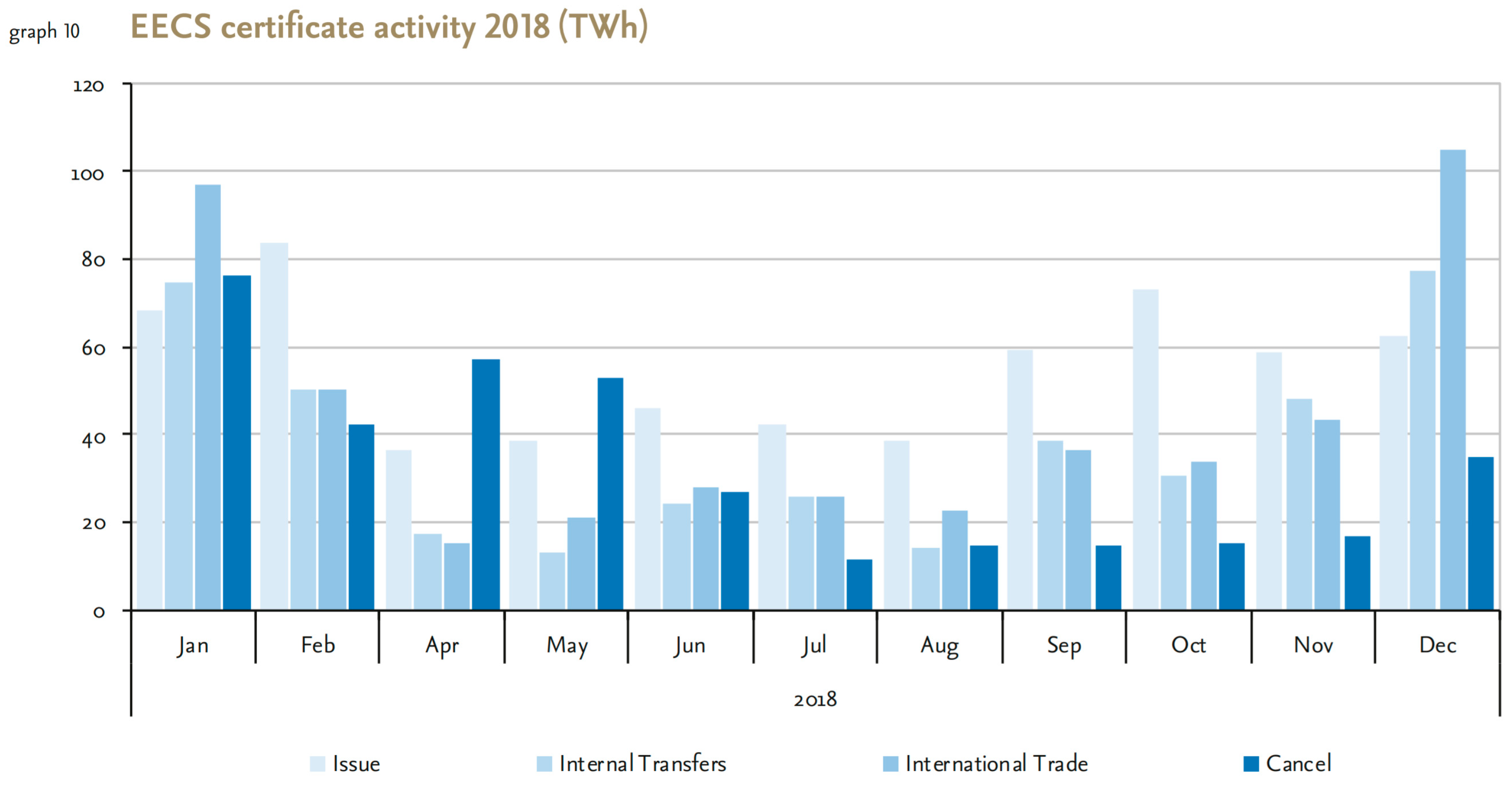
Figure 3 of this paper. This figure indicates 48.82% of redeemed certificates from the total of issued certificates. Given the reference values in Portugal, presented in
Table 1, which set the base values to pay for each certificate issued and redeemed, we get a reference value for the sale of such certificates: 4.8165 c€/MWh, obtained by multiplying the issue price of 10 c€/MWh by 48.82%. For each kWh produced from renewable energy sources, the observed gain in the Guarantees of Origin certificates market corresponds to 0.0048165 c€, a much lower value than the gains obtained by acting on the carbon market.
This strategy consists in presenting the bids for the electricity market, as the value obtained by subtracting the value gained by the sale of guarantees of origin certificates to the initial price proposed by Seller 2. To test this strategy, we present two simulations undertaken using MASCEM. In the first simulation are considered the values obtained from MIBEL, where Seller 2 original bid prices were kept constant, and the supply of energy production is set at 100 MWh. The second simulation considers the same scenario, however, this time Seller 2 bid prices are defined by the strategy mentioned before: subtracting the income from the participation in the Guarantees of Origin certificates market to the original bid price.
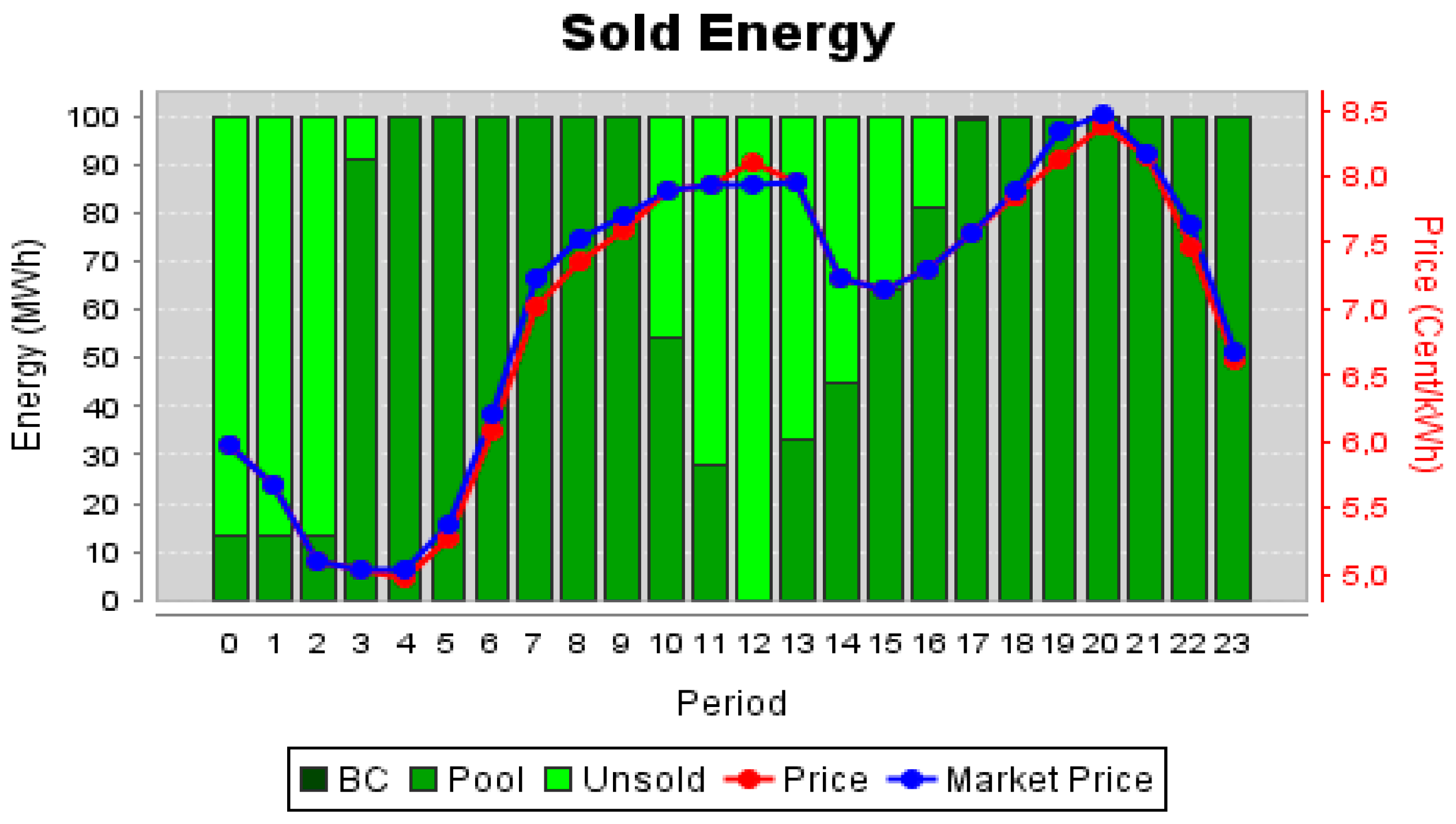
Figure 8 presents the market results for Seller 2, in the case of not participating in the Guarantees of Origin certificates market.
From
Figure 8 one can observe that the Seller 2 managed to sell most of the available energy. There were only a few periods when this player could not sell some energy, being period 12 the only one when the value proposed by this player was above the market price, implying that it has not sold any energy in that period. This means that the offers did by this seller have an important influence in the market prices in most of the periods.
The success or failure in selling depends on the competitiveness of the bid price proposed by the player. A seller that can present low bid prices has much higher chances of selling than a player that is forced to present high prices. However, it must be noted that a player must always present bids that allow it to cover its expenses (fixed and variable) and still obtain some profit. Therefore, for a player to be able to present lower proposals than its competitors it must get a strategic advantage somehow, e.g. from entering parallel markets, which allow the achievement of extra ordinal incomes.
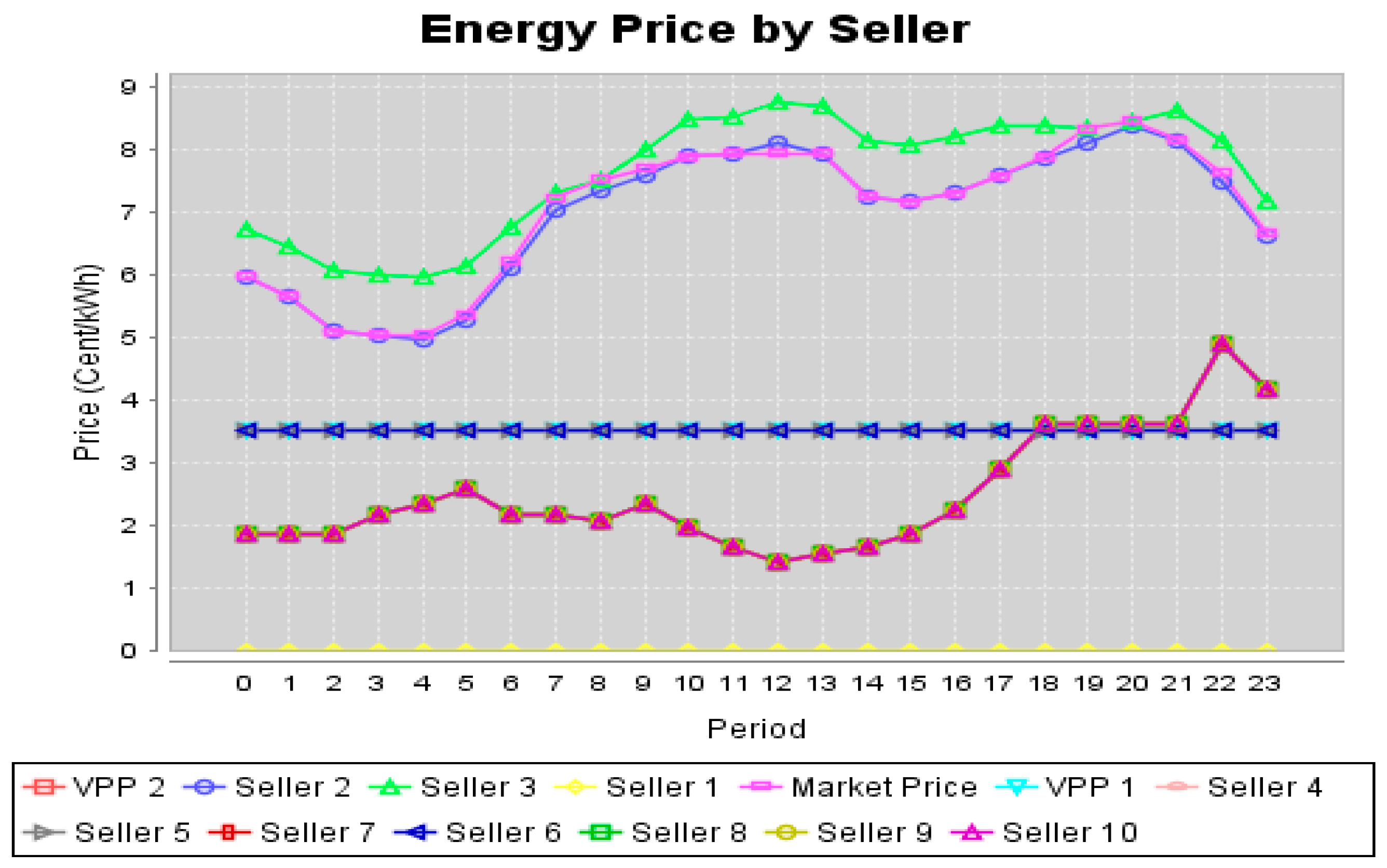
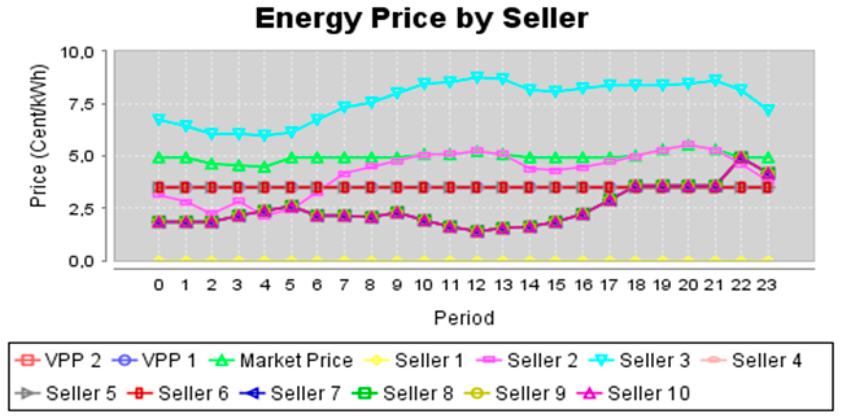
Figure 9 presents the evolution of all sellers’ proposals throughout the day.
From
Figure 9 it is visible that the bid price of Seller 2 is highly competitive with some other sellers. This is almost unnotable by the overlapping of the curves of the graph. This competition, and proximity in bid prices, indicates that a small reduction in the bid price from behalf of Seller 2 can mean a notable difference in what concerns the market sales results.
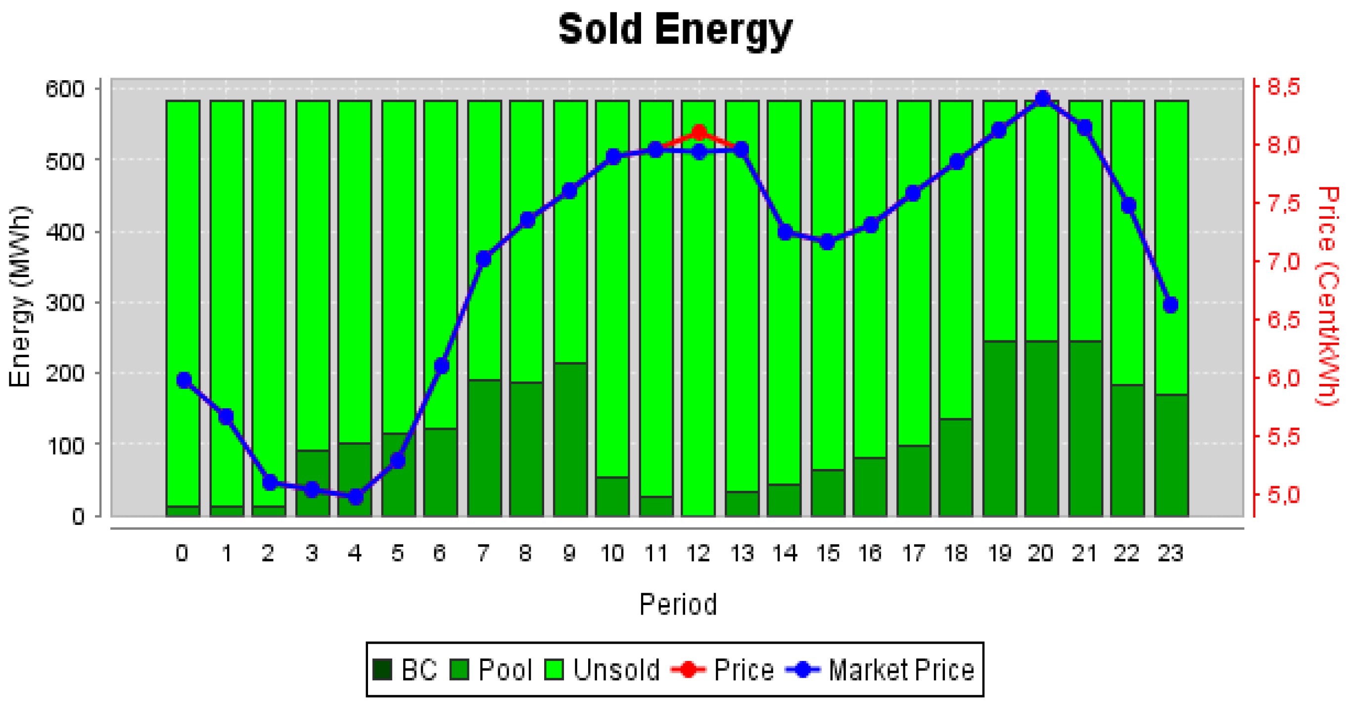
Figure 10 and
Table 2 aim to demonstrate the values obtained with the second simulation, considering the gain obtained in the Guarantees of Origin market, in the definition of the offer made on the second day.
From
Figure 10, and comparing it with
Figure 8, it is visible that despite the participation in the market for Guarantees of Origin certificates the values acquired by the sale of certificates do not allow Seller 2 to sufficiently decrease its bid price, to increase its energy sales in the market.
Table 2 presents the electricity and Guarantees of Origin markets results. The first column shows the base values initially imposed by Seller 2 in c€/kWh, having 100 MW to sell in every hour. The values of the last column represent the gain obtained in the Guarantees of Origin market, which are subtracted from the original offer.
The second simulation shows that Seller 2 failed to sell more energy when participating in the green certificates market because its gains in the Guarantees of Origin market have not been enough to make a more attractive offer in order to sell a higher amount of energy. The energy that was actually sold can be found in the third column of
Table 2.
The conclusions drawn by the strategy for the involvement of energy producer in the market for licenses are quite clear according to the data from the presented simulations. It appears that the registered producer cannot gain enough in the Guarantees of Origin market to significantly lower its bid in the sale of electricity.
The failure to obtain larger profits from the sale of Guarantees of Origin certificates does not mean that companies involved in the production of energy using renewable sources should not have some facilities registered in this system. Despite the incomes from the selling of Guarantees of Origin certificates not being high, they still mean an extra revenue. And even this strategy can show different results when the original bid prices are even closer to the market price, which can be achieved with the use of forecasting and data mining methods. In that case, even a minimal reduction in the prices can be translated into an increase in the amount of selling power, and consequently the increase in profits.
In order to complement the analysis made for the two reference days presented in the above simulations,
Table 3 presents a sensitivity analysis on the influence of the sold volume and reference price for selling of Guarantees of Origin certificates. This analysis presents the extra revenue (in €) obtained by selling Guarantees of Origin certificates during a full day, assuming the same availability of 100 MW in each hour. The sensitivity analysis considers different variations of the total volume of sold energy during the day, and variation of the reference price of Guarantees of Origin certificates depending on the percentage of redeemed certificates.
From
Table 3 it can be seen that the extra revenue obtained by selling Guarantees of Origin certificates can be up to 2400.00 € in the total of the considered day. This scenario considers that 100% of the submitted certificates are redeemed and the total volume of energy is sold throughout the entire day. Although this is currently not a realistic scenario, it may be not that far away. Given the current agreements and initiatives to boost the usage of renewable energy, it is not unfeasible that in some years all the certificates may possibly be redeemed. Even when considering a percentage of 50% redeemed certificates: the reference value identified by this study given the current status of the Guarantees of Origin trading, the extra revenue obtained when selling the entire amount of energy is of 1200.00 €, which is still a very significant amount as additional daily income on top of the energy sale in the wholesale electricity market. In summary, it is noteworthy to mention that the participation in Guarantees of Origin certificates trading is always beneficial for renewable energy sellers, as it represents an additional gain that complements the incomes from the traditional electricity market participation.
4.2. Strategy 2: Participation in the Carbon Market
A seller’s participation in the carbon market allows a possible selling of emission rights if it can manage to stay under the maximum of granted allowances. The strategy is defined by a reduction in power production in order to be able to obtain credit in the carbon market, this way being able to sell the exceeding allowances in the CO2 emissions market, gaining room to reduce the value of its bid in the energy market, if the producer finds that it is not obtaining a significant dispatch of the selling power.
Technologies based on fossil fuels as a source of production have a higher rate of emissions. This requires greater care in the management because what may be looked at as profit in the electricity market may have additional costs in the case of having to pay high values for exceeding the awarded allowances.
To test this strategy, we will maintain the bid values for the first day constant. If Seller 2 can not sell all of its power at the desired price, the next day’s bid will be lowered in accordance to the profits obtained the day before in the CO
2 emissions market. The next example aims to demonstrate this strategy more explicitly. In this study, Seller 2 represents a producer that explores the Pego Thermal Power Plant in Portugal (
http://www.tejoenergia.com/):
Allowances per year: 2,723,011 tonCO2;
Installed capacity: 584 MW.
Consideration: The plant ceases to produce during 48 h to be able to acquire enough allowances to cover emissions made in the third day, therefore lowering its required price in the energy market. To cover the CO2 emissions recorded during energy production, the producer will have to use the allowances acquired in previous days and sell those in excess in the carbon market. The value gained in this operation will be applied in the reduction of the bid for the electricity market.
Considering a total allowance per year and an average generation of 584 MWh, means that, approximately, 479.60 tonnes of CO
2 per hour will be issued representing an allocation of allowances of 310.85 tonnes of CO
2 per hour. This means the producer would have to buy licences to compensate for the issued excess. However, since it did not produce energy during 48 h, it gained a total value of € 179,049.60 with the sale of the allowances it saved during those hours, considering as reference the value of € 12 per allowance presented in
Section 2.2. In the third day, the total amount of allowances needed per hour to compensate for the extra production is the hourly allocation of allowances (310.85 tonCO
2) subtracted to the effective hourly production (479.60 tonCO
2) corresponding to 168.75 tonCO
2. This means an hourly expense of € 2025.00 and a total expense for the day of € 48,600.00. Therefore, the total profit, €130,449.60 is the total income received from the selling of the allowances in the first 48 h, without the total value paid to compensate for the extra production in the last day. Now, if we divide this total profit for the total production of the day, we get to the value that we can subtract to the bid to still maintain the guarantees of having profit. This corresponds to 0.9307 c€/kWh in the possible reduction of Seller 2′s offer in the energy market.
This means the producer would have to buy licences to compensate for the issued excess. However, since it did not produce energy during 48 h, it gained a total value of € 179,049.60 with the sale of the allowances it saved during those hours, considering as reference the value of € 12 per allowance.
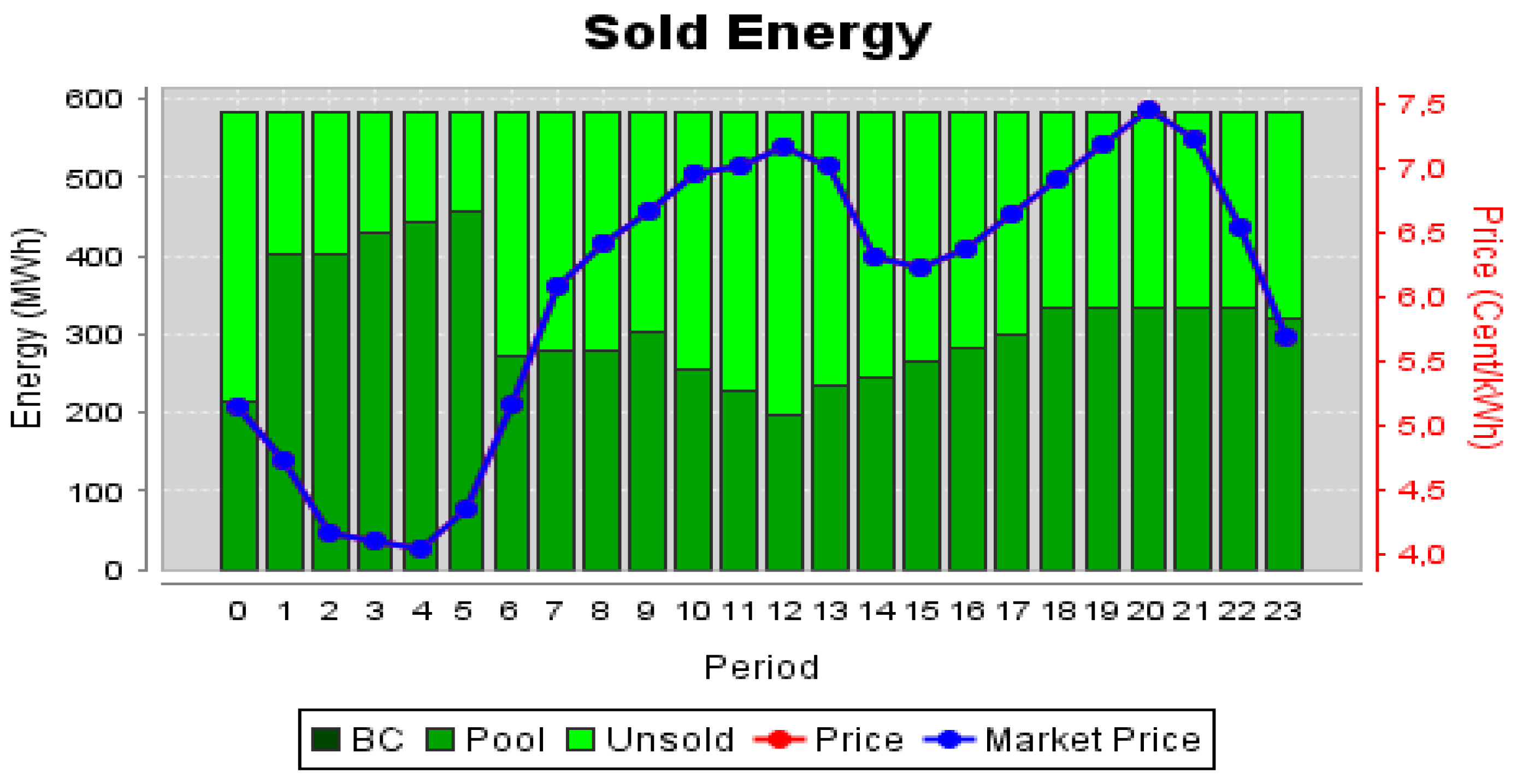
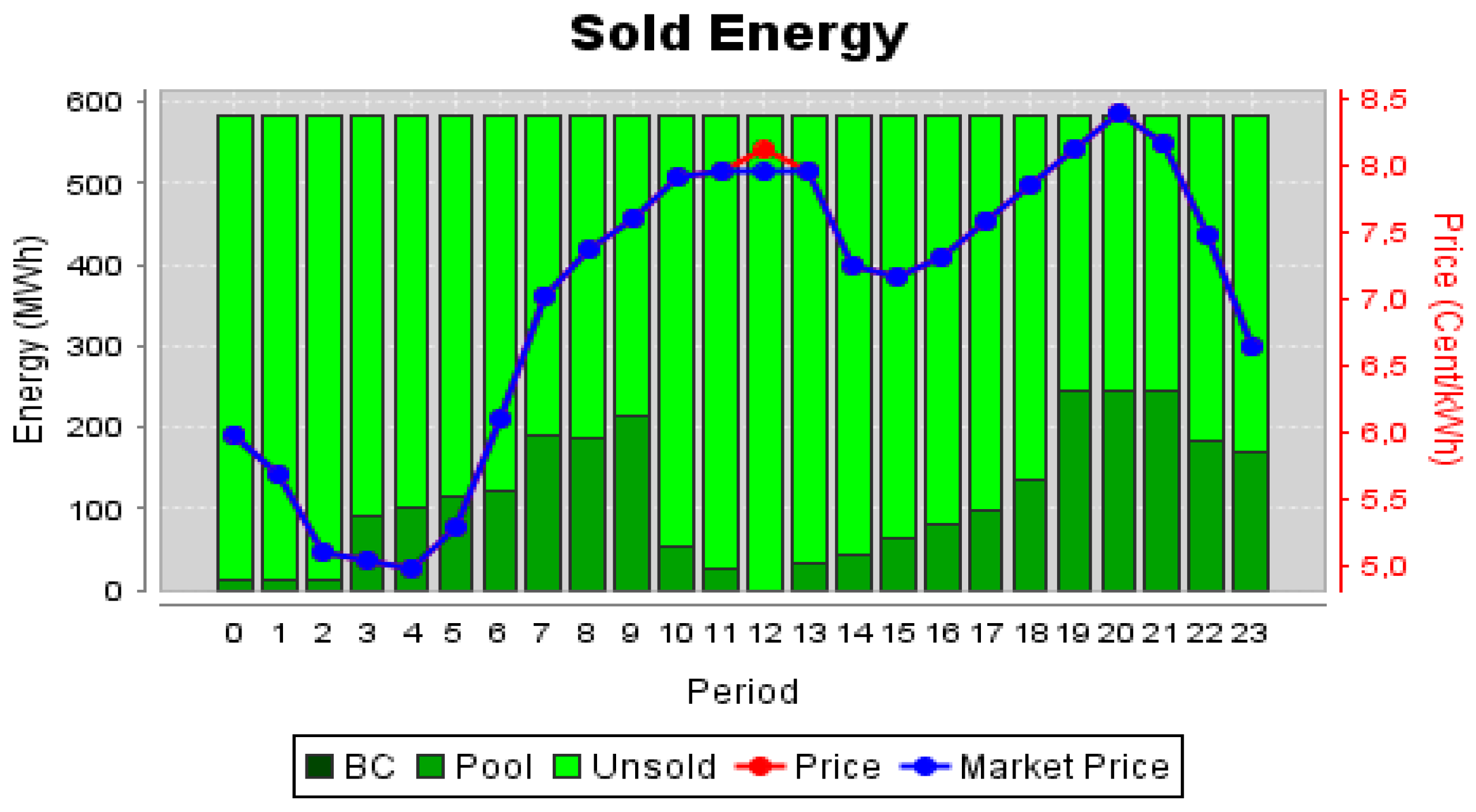
The simulation that follows is performed with MASCEM and intends to demonstrate the change in energy sales in the market over 24 h. On the first day, the gain realized on the carbon market is not considered, while the offer of the following day takes into account the profit of the previous days.
Figure 11 presents the results of Seller 2 when acting in the electricity market for the first day (without considering the gains in the CO
2 emissions market yet).
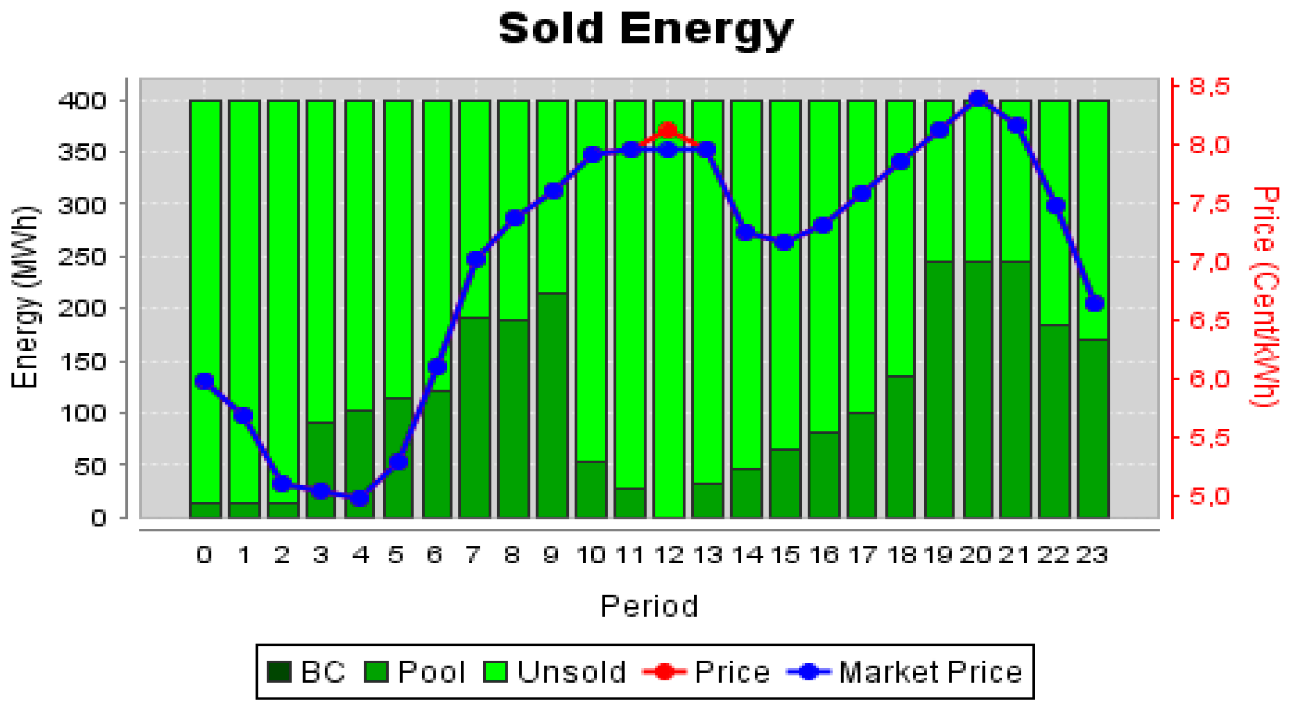
Figure 12 presents the results of Seller 2 for the second day, when acting in the electricity market considering the gains in the CO
2 emissions market achieved in the previous days.
Figure 11 and
Figure 12 allow observing the amount of energy sold in the market. The dark green bars represent the energy that was actually sold, compared to the base production, the blue line represents the market price set by the market operator, and the red line represents the bid price set by Seller 2.
Seller 2 has stopped its production for two days allowed it to get enough credits to cover the license issued by energy production and to define a more attractive offer which is reflected in the amount of energy it could sell. The fact that the blue and red lines are overlapped in most periods in both graphs is a result of Seller 2 being the most influent seller in this simulation, and its bid price is defining the market price in most periods. This is the main reason why this was the chosen seller to be our object of study, this way it is possible to have an easier visualization of the changes that happen when its bid price and energy amount change.
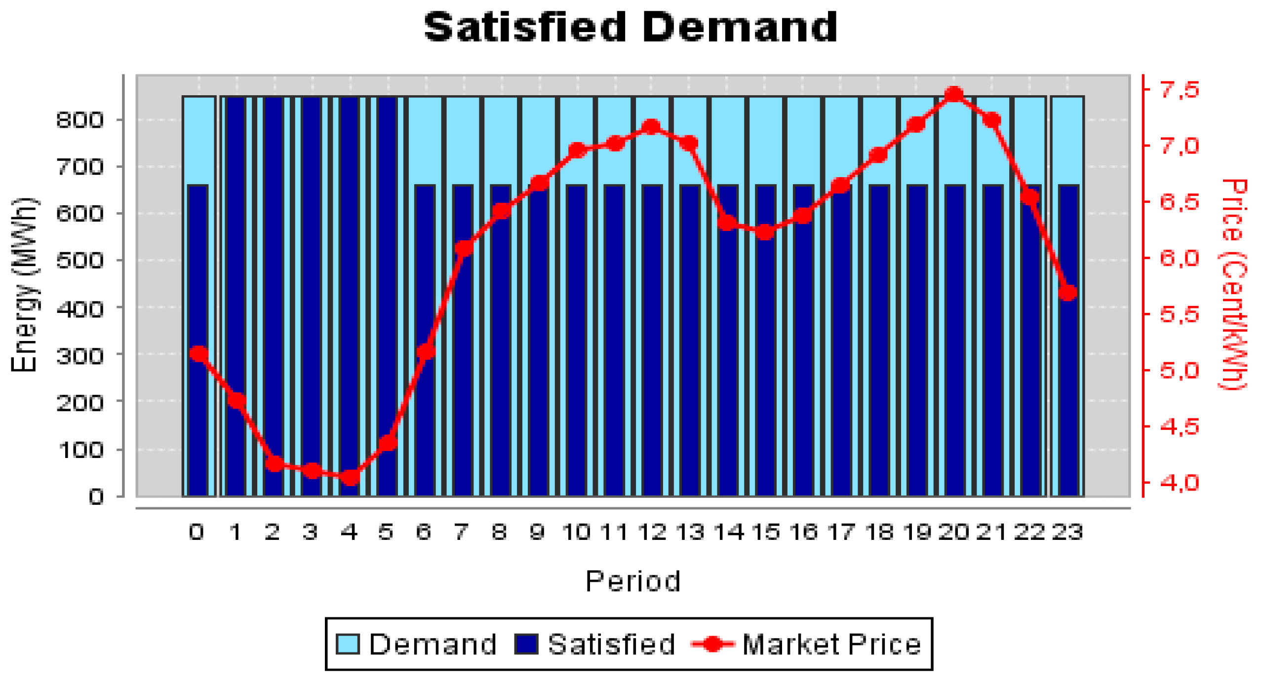
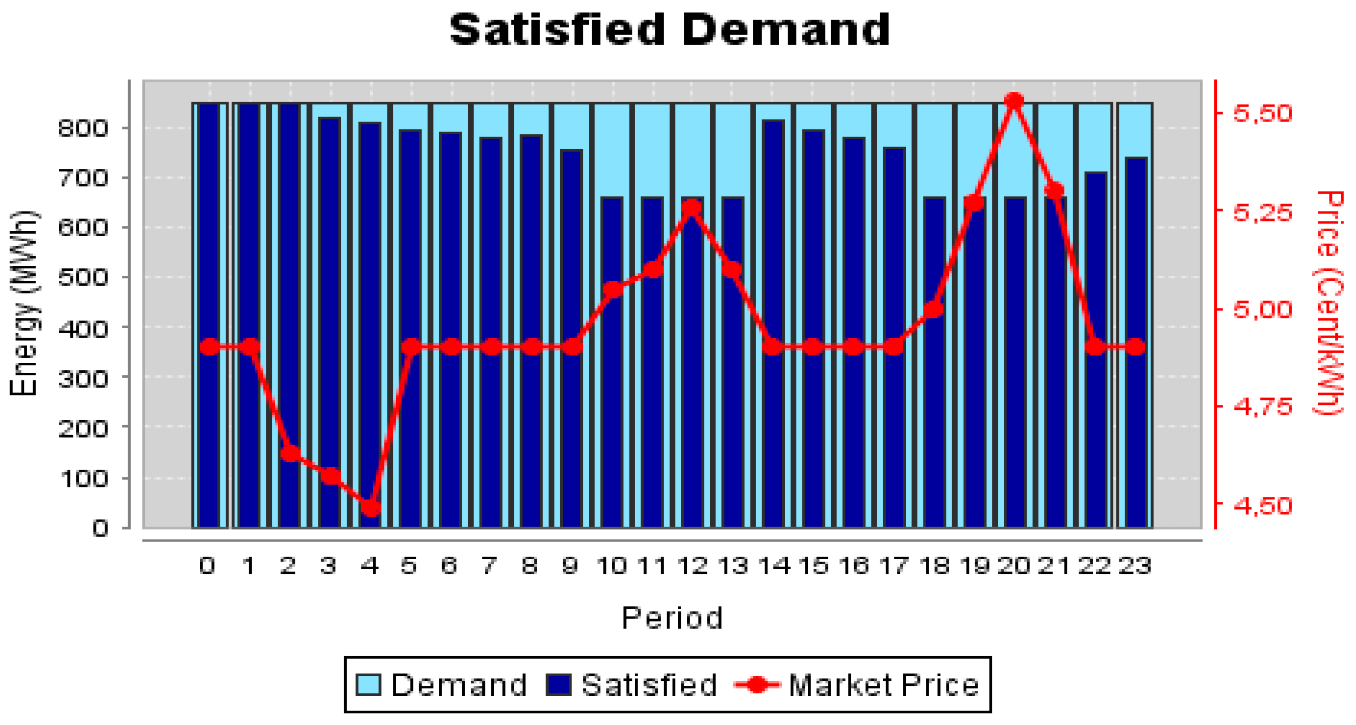
Figure 13 presents the comparison between the total demand in the market and the demand that was, in fact, satisfied.
Depending on the variation in energy prices imposed by the market, it is observed if the demand for energy was satisfied or not. The graph of
Figure 13 is characterized by the results obtained with Seller 2 participating in both the electricity market and the CO
2 emissions market.
Figure 13 shows that Seller 2′s decrease in its bid originated the satisfaction of much of the energy demand.
Table 4 presents a comparison between the proposed and accepted bids for Seller 2, in both cases, with and without the carbon market participation. From
Table 4 it is important to note the results obtained with the action in the carbon market, being Seller 2 a facility registered in the EU-ETS and adopting the proposed market strategy, it can be observed that in the first simulation (offer
n) were sold only 2689 MW over 24 h. In the second simulation (offer
n + 1) the sale struck up the 7477 MW, about 64% more.
According to the values recorded in the table, it is possible to see that Seller 2, by acting in both the carbon market and electricity market can obtain a total of € 441,737.91. This is a high value compared to the € 195,161.02 obtained without the simultaneous participation in the two markets. Now, let’s analyze the case where Seller 2 does not participate in the CO
2 market at all.
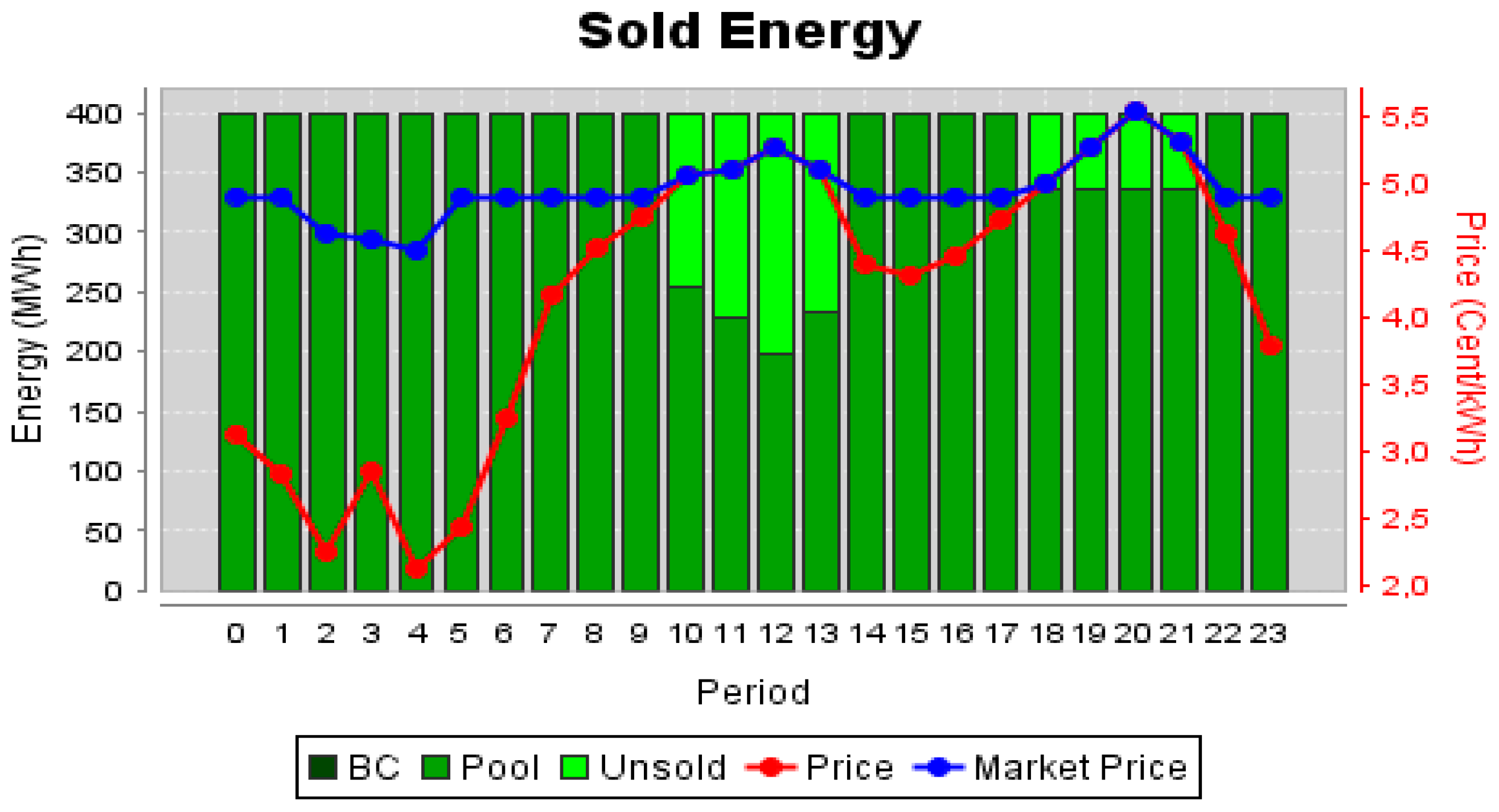
Figure 14 shows the simulation values for the first day of simulation.
The difference from the case presented in
Figure 14 to the first day of the previous simulation (
Figure 11) is that since there was no stop in production, the amount to pay for CO
2 emissions will affect the offer made to the market, implying its increase to try to regain some of the money spent to buy emission allowances.
Table 5 shows the influence of the buying of allowances in the bid price of Seller 2.
According to the values shown in
Table 5, when the facility produces 584 MWh during 24 h, it emits about 479.60 tonnes of CO
2 per hour, an amount that exceeds the average 310.85 assigned to it. As it cannot stay below the allocations, it will have to buy allowances amounting to € 4050.10, which is the difference between the emissions recorded and allocated, multiplied the average value of € 12 per tonne of CO
2. With these data, it is estimated that the producer will have to pay approximately 0.6935 c€/kWh per hour. This value will be considered in the offer price of Seller 2 in the market.
Table 5 shows the value that the power producer will have to pay for emitting more CO
2 than what is allowed. The considered amount of energy to sell on the market was 584 MWh. However, the value actually sold is far below, which allows us to infer that the fact that it increased the offer price has not contributed to the selling of a large part of the energy. Values with negative sign mean prejudice to the power producer, as it will have to recover the money lost in the carbon market. The values of the first column of the table are determined to take into consideration the values of the last column.
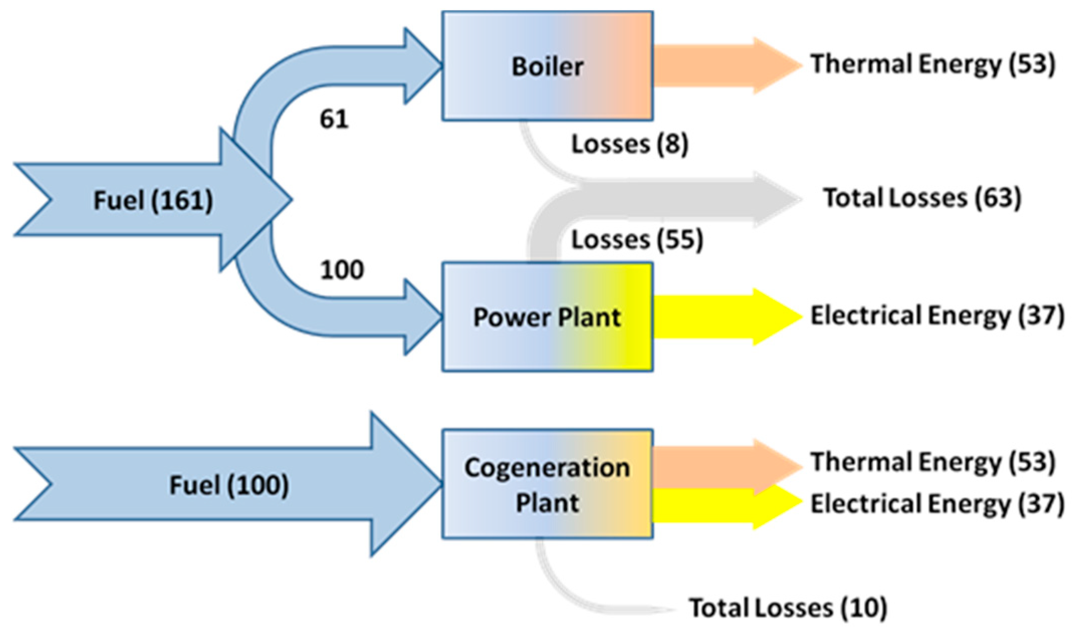
4.3. Strategy 3: Participation in the Hot Water and Steam Market
Strategy 3 considers the sale of steam produced by a cogeneration plant with an installed capacity of 400 MW. The remuneration from the sale of steam will be critical to enable Seller 2 to formulate offers below the price imposed by the market operator, to increase its odds to sell as much of the electricity produced in CHP plant as possible.
The remuneration gained with the sale of steam for each kWh of electricity produced is 2.85 c€. This value will allow Seller 2 to revise its bid on the second day of action in the electricity market. Similarly, to the previous strategies, two simulations will be presented for different days, the first simulation considers the bid prices without reducing the bid for the electricity market, based on the profit gained in the market for steam. The second, on the contrary, takes into account the value of 2.85 c€ per hour obtained by the sale of steam.
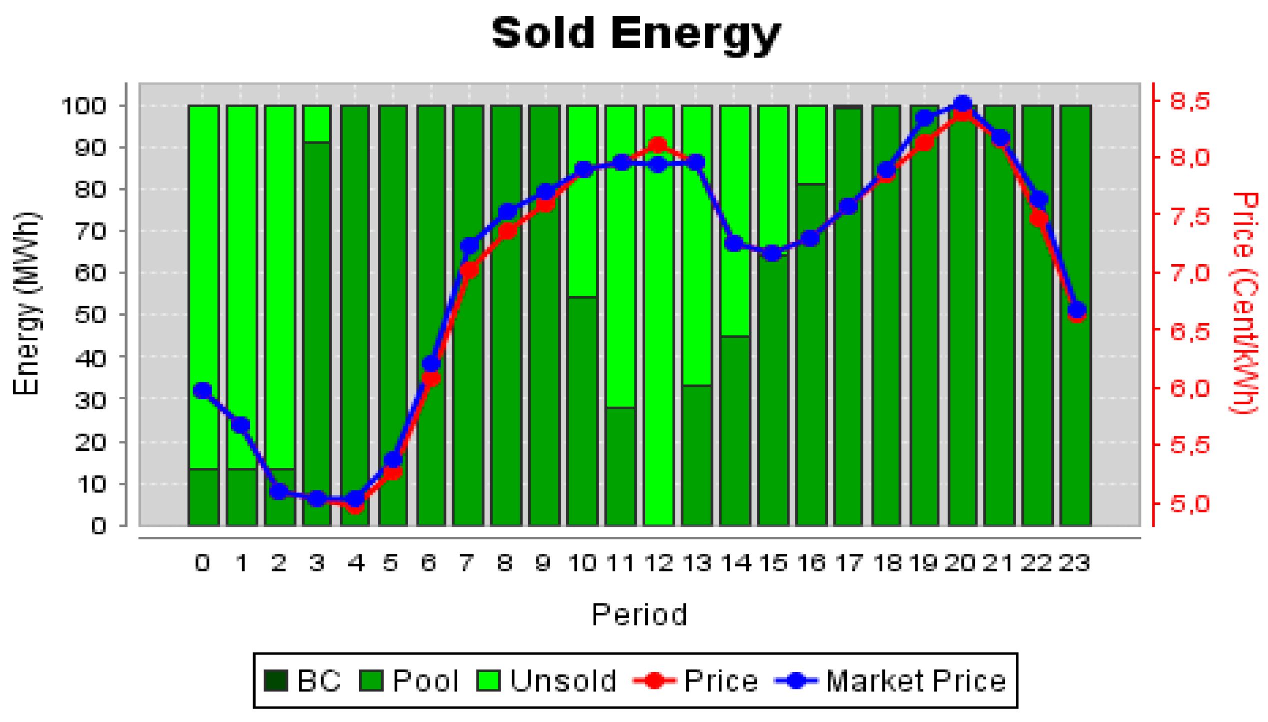
Figure 15 shows the results for Seller 2 when participating in the market, when not considering the participation in the steam sale.
The chart presented in
Figure 15 shows the maximum energy that Seller 2 desires to sell, the price at which energy is sold and the amount of energy that is actually sold.
Figure 16 shows the same information for the case of the profits with the steam sale being considered.
Analysing
Figure 16 it is obvious that the results for this second case are much more advantageous for Seller 2. The reduction in the bid price allowed Seller 2 to sell practically all its available energy in every period. By showing the comparison between all sellers’ proposals in the electricity market,
Figure 17 shows how the reduction in Seller 2′s bid price influenced the market results.
From
Figure 17 one can see how Seller 2′s bid prices compare to the other sellers’ bids, enabling it to stay always bellow the market price, and therefore sell all of its available power at a higher price, except from periods 10 to 13. These simulations allow showing the success achieved by Seller 2 in the sale of most of the available energy. These results were possible only because of the profit gained with the sale of steam.
Figure 18 presents the comparison between the total demand in the market and the demand that was, in fact, satisfied.
One can see in
Figure 18 that Seller 2′s success also contributed to the almost total satisfaction of the market demand for this day.
Table 6 shows the results for Seller 2 when performing the steam sale. By
Table 6 one can see the gains achieved with the proposal for the first day (day n), values not considering the sale of steam; and the values won with the bid for the second day when the bid is reduced by a value of 2.85 c€, compared to the previous days, guaranteed by the sale steam. The bid for the second day (
n + 1) is far more profitable for Seller 2 because it allowed the sale of more 5964 MW of energy than in day n. The total gain obtained by acting in the steam market is valued at € 351,705.14 while considering the offer
n, the total gain would be only € 195,161.02.
Table 7 presents a sensitivity analysis on the influence of the steam market price and traded volume over the expected revenues of the player. This analysis considers as reference steam market price the 2.85 c€/kWh explained above (100%), and analyses the impact of the variation of this price up to 50% upwards and downwards. It also considers the influence of the traded volume, from 0% to 100% trading success.
From
Table 7 one can see that the additional gain is high regardless of the producer’s generated amount. Since the steam can be sold in a complementary way to the electrical energy, generators can find a significant source of additional revenue with the sale of the water steam. The steam price variation has an obvious influence on the additional revenue that can be achieved, but this income is relevant even when the price drops to one half; hence suggesting that the participation in the water steam market should not be neglected.


