Effect of Multi-Factor Coupling on the Movement Characteristics of the Hydraulic Variable Valve Actuation

Abstract

Studies show that the valve lift (VL) of the cam-driven hydraulic variable valve actuation (VVA) can be continuously adjusted in the range of 0–8.2 mm by controlling the opening of the throttling valve. In the present study, an orthogonal experiment with interaction was designed to analyze the effect of multi-factor coupling on the VL, valve-seating velocity (VSV), and pressure fluctuation in the valve piston cavity. In order to reduce the pressure fluctuation, the Taguchi method was applied to find the optimal combination of the key parameters including the diameter of the piston, the spring preload of the valve-seating buffer mechanism (VSBM), the spring preload of the valve, and the valve piston mass. The correctness of the VVA simulation model is verified through experiments. Moreover, the pressure fluctuation is analyzed through a numerical simulation. The obtained results showed that as long as the VSV is less than 0.5 m·s⁻¹, the pressure fluctuations in hydraulic VVA can be reduced by several means, such as increasing the spring stiffness of the VSBM and valve, increasing the valve piston area and diameter size of the thin-walled hole, and reducing the valve piston mass and total hydraulic oil volume.

1. Introduction

In recent years, increasingly stringent fuel consumption and pollution emission regulations have brought unprecedented challenges to the automotive industry. Therefore, many companies have adopted advanced technical methods to improve engine efficiency [1]. Studies show that the application of increasingly flexible and variable valve systems can improve the Miller cycle, reduce the pumping loss of the part-load on the gasoline engine, and improve the thermal efficiency and fuel economy [2,3]. Wang et al. found that the gasoline-fueled Miller cycle exhibited higher engine efficiency by up to 6.9% at an indicated mean effective pressure (IMEP) of 7.5 bar [4]. Li’s research found that when the Miller cycle was used, the indicated specific fuel consumption (ISFC) was reduced by 11% relative to the ISFC of the original engine [5].

The variable valve actuation (VVA) is mainly divided into three categories, including the mechanical, electromagnetic, and electro-hydraulic types [6,7,8]. The mechanical type has high reliability and control accuracy. However, the adjustment degree of freedom in this scheme is low so that the flexibility is limited [9,10]. On the other hand, the electromagnetic type has functional shortcomings such as problems associated with motion control. Meanwhile, the response frequency of the solenoid valve limits the maximum speed of the engine [11,12]. Moreover, the electro-hydraulic type has superior characteristics, including flexible mechanism configuration, high system rigidity and fast response [13,14,15]. It is worth noting that the 1.4 L MultiAir engine developed by the Fiat company is driven by an electro-hydraulic valve mechanism, where the rated speed of the engine is 5500 rpm. Studies show that the fuel consumption of this engine reduces by 7.6%, when compared to conventional engines [16,17]. Wei et al. produced a prototype that can realize the throttle control of gasoline engines without throttling [18]. Hu et al. reduced the ${\mathrm{NO}}_x$ emissions of diesel engines through the continuously variable valve lift (VL) mechanism [19]. These achievements indicate that the electro-hydraulic variable valve has reasonable application prospects.

The electro-hydraulic VVA involves multiple hydraulic components. When the hydraulic system is working, the multi-factor coupling effect imposes pressure fluctuations on the system [20,21]. These pressure fluctuations can cause vibration, noise, and fatigue failure of hydraulic components in hydraulic systems, thereby reducing the service life of the workpiece and the overall performance of the engine [22]. Han et al. analyzed the transient pressure of the hydraulic oil circuit of the electro-hydraulic VVA and studied the influence of the opening slope of the return solenoid valve on the system pressure [23]. Xie et al. reduced the hydraulic fluctuations effectively in the VVA by improving the quality of moving parts and designing the valve cam profile [24]. Furthermore, Zhong et al. analyzed the effects of different engine speeds and throttle openings on the pressure fluctuations [25].

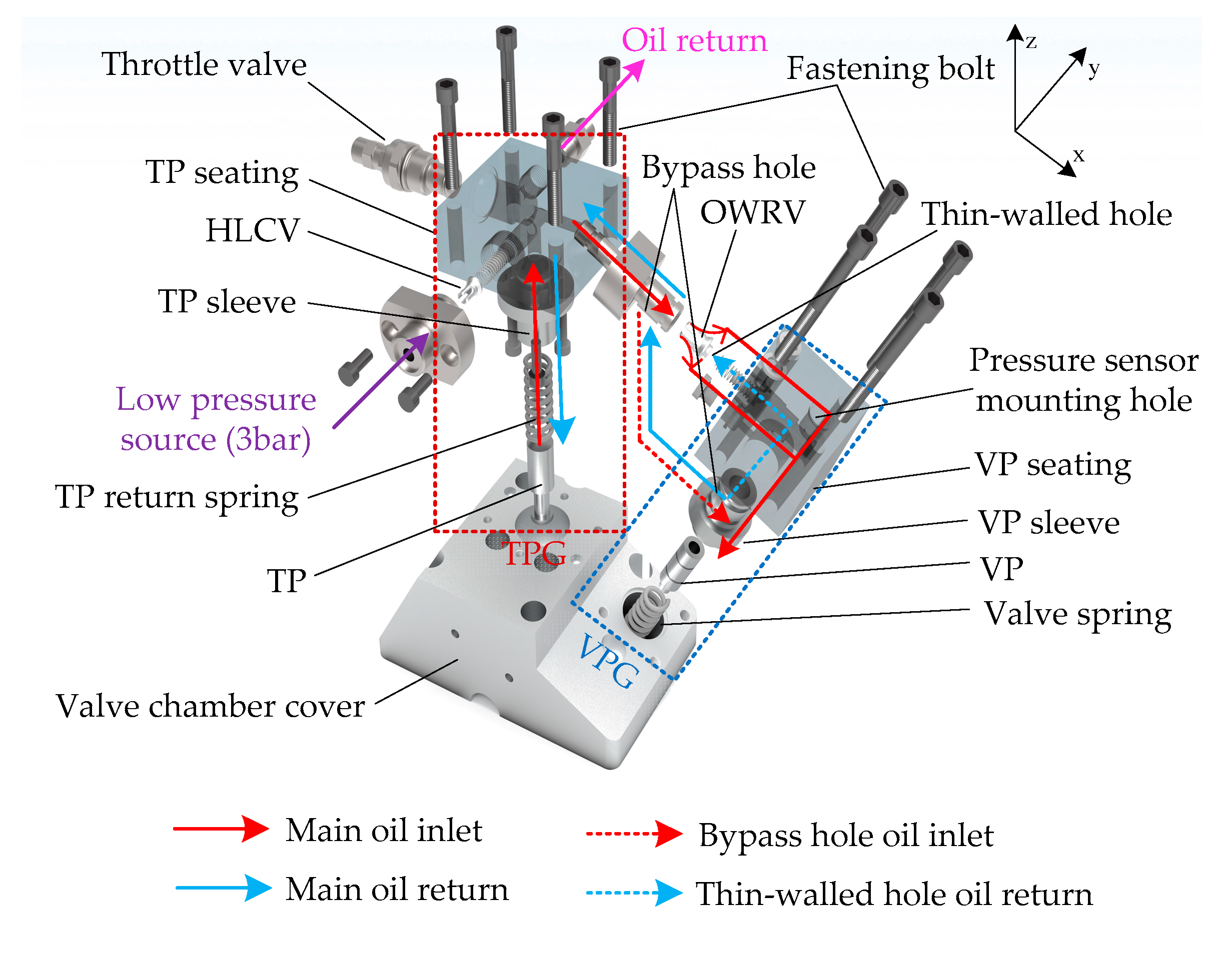
It is worth noting that the electro-hydraulic VVA is limited by space and compact structure. However, structural parameters such as the tappet piston, valve piston, and pipe diameter play a key role in the valve performance. Moreover, the valve spring preload and rigidity, the valve piston quality, and the diameter size of the thin-walled hole of valve-seating buffer mechanism (VSBM) components also have a remarkable impact on the vibration and pressure fluctuation of the hydraulic system. In the present study, these parameters were analyzed through numerical simulations and experimental study. Moreover, solutions to reduce the pressure fluctuation were obtained successfully.

The Taguchi method is utilized widely in the design and analysis of the experimental method to optimize the performance characteristics through the setting of process parameters. Based on orthogonal arrays, the number of experiments, which may lead to an increase in time and cost, can be reduced by using the Taguchi method. It employs a specific design of orthogonal arrays to learn the full set of parameters by performing the least number of experiments only. Interaction problems are often encountered in the orthogonal experiment [26,27,28]. Feng et al. performed the multi-objective optimization of the forging process parameters on the helical gear precision by using the Taguchi method. They determined the optimal combination of process parameters through the modified Taguchi method [29]. Shin and Lee studied the accelerated condition of the brush wear on a small brush-type DC motor by using the Taguchi method and analyzed the impact of various factors to assess the influencing potential of important factors accurately, objectively, and quantitatively on data [30]. Accordingly, they demonstrated that the orthogonal experiment could be used to analyze the effect of multi-factor coupling on the VVA, thereby seeking the optimal combination of key parameters through the Taguchi method.

In the present study, a cam-driven hydraulic variable valve actuation (CDH-VVA) was designed. By controlling the opening of the throttle valve, the VL acted as a continuous variable. Moreover, the mathematical model of the CDH-VVA was established and the transfer function of the throttle opening to the VL was derived. The influence of the dynamic characteristics and main performance parameters of the hydraulic power components in the system on the VL was analyzed. Moreover, the AMESim simulation model was established. Then the correctness of the simulation model was verified through the test. An orthogonal experiment with interaction was designed in this regard. Furthermore, the effect of multi-factor coupling on VL and pressure fluctuations was investigated through the Taguchi method to obtain the optimal combination of horizontal factors. For better space layout, the valve-seating velocity (VSV) and the pressure fluctuation were reduced. The effect of the key parameter coupling on the hydraulic VVA was studied through further simulation analysis. Measurements for reducing the pressure fluctuation were finally proposed.

2. Research Basis

2.1. Principle of the CDH-VVA

Figure 1 shows a three-dimensional model of the CDH-VVA, which consists of a tappet piston group (TPG) and a valve piston group (VPG). The external system utilizes a hydraulic station as a constant low-pressure source (3bar) to refuel the system. The tappet piston (TP) is driven upward by the cam rotation. When the high-low check valves (HLCV) are closed, the tappet piston cavity (TPC) gradually increases the pressure, and the high-pressure oil pushes the valve piston (VP) open through the connecting oil passage. In the early stage of the valve opening, the high-pressure oil overcomes the spring preload of the one-way restrictor valve (OWRV) to open it. Then, the high-pressure oil enters the valve piston cavity (VPC) from the main oil inlet to overcome the valve spring preload (VSP) and pushes the valve open. When the valve is opened 2 mm, the VP bypass hole gradually opens, and the high-pressure oil enters the VPC through the connecting oil channel bypass hole, pushing the valve to reach the maximum VL. When the cam turns over the sharp angle, the system pressure begins to decrease. Under the VSP, the valve starts to return. At the initial stages of pressure drop, the hydraulic oil returns to the TPC through the valve piston bypass hole. In the backward period, before the VP returns to the valve seating at the remaining 2 mm, the bypass hole of the VPC is covered and closed by the VP. The hydraulic oil returns to the TPC through the thin-walled hole. Then, the opening of the throttle valve is adjusted to change the effective flow area, and realize the continuous variable VL.

2.2. Mathematical Model of the System

Figure 2 shows the schematic configuration of the system. Based on the force of the valve piston, the momentum equation can be expressed as follows:

$$p_2{A}_2=m_2\frac{d^2{h}_2}{d{t}^2}+F_q+G{h}_2+B_p\frac{d{h}_2}{dt}$$

(1)

where $m_2$ is the mass of the VPG, $h_2$ is the VL, $p_2$ is the pressure of the VPC, $A_2$ is the area on the top of the VP, $F_q$ is the VSP, $G$ is the valve spring stiffness, and $B_p$ is the motion damping coefficient of the VPG. It should be indicated that the gravity $m_{2}g$ of the VPG and the friction force $F_{r2}$ are relatively small compared to the hydraulic pressure, so that they are ignored in the momentum equation.

The flow continuity equation of the TPC can be mathematically expressed as follows:

$$A_1\frac{d{h}_1}{dt}=Q_1+Q_L+c_1{p}_1+\frac{V_1}{\beta }\frac{d{p}_1}{dt}$$

(2)

where $A_1$ is the area on the top of the TP, $Q_1$ is the flow to the VPC, $Q_L$ is the flow of the throttle valve, $c_1$ is the leakage factor of the TPC, $p_1$ is the pressure of the TPC, $\beta$ is the fluid compressibility, and $V_1$ is the instantaneous volume of the TPC.

The flow continuity equation of the VPC is:

$$A_2\frac{d{h}_2}{dt}=Q_1-c_2{p}_2-\frac{V_2}{\beta }\frac{d{p}_2}{dt}$$

(3)

where $A_2$ is the area on the top of the VP, $Q_1$ is the flow to the VPC, $h_2$ is the VL, $c_2$ is the leakage factor of the VPC, $p_2$ is the pressure of the VPC, $V_2$ is the instantaneous volume of the TPC, and $\beta$ is the fluid compressibility.

The volume of the TPC and the VPC is very small; therefore the compressibility of the liquid in the cavity is ignored. Combining Equations (2) and (3) yields the following expression:

$$Q_L=A_1\frac{d{h}_1}{dt}-A_2\frac{d{h}_2}{dt}-c_1{p}_1-c_2{p}_2$$

(4)

The linearized flow equation of the throttle valve is:

$$Q_L=K_{q}X+K_c{P}_L$$

(5)

where $K_q$ is the flow gain, $K_c$ is the flow-pressure coefficient, $X$ is the throttle opening, and $P_L$ is the throttle load pressure.

Applying the Laplace transform on Equations (1), (4) and (5) results in the following expressions:

$$\{\begin{array}{c}{p}_2=\frac{m_2}{A_2}{s}^2{h}_2+\frac{B_p}{A_2}s{h}_2+\frac{G}{A_2}{h}_2+\frac{F_q}{A_2}\\ Q_L=A_{1}s{h}_1-A_{2}s{h}_2-c_1{p}_1-c_2{p}_2\\ Q_L=K_{q}X+K_c{P}_L\end{array}$$

(6)

The transfer function of the $h_2$ is defined as:

$$h_2=\frac{A_1{A}_{2}s{h}_1-A_2{c}_1{p}_1-A_2{K}_{q}X-A_2{K}_c{P}_L-c_2{F}_q}{m_2{c}_2{s}^2+(B_p{c}_2+A_2^2)s+G{c}_2}$$

(7)

The transfer function of the X, which is an input, is expressed as:

$$\frac{h_2}{X}=\frac{-A_2{K}_q}{m_2{c}_2{s}^2+(B_p{c}_2+A_2^2)s+G{c}_2}$$

(8)

Equation (7) indicates that the top area of the TP and the VP, the pressure of the throttle valve and the VSP affect the size of the VL. The characteristic equation shows the variations in the piston mass, spring stiffness, and leakage of the valve.

3. Simulation Model and Test Verification

3.1. AMESim Simulation Model of the CDH-VVA

Multiple factors affect the system, thus it is of significant importance to minimize the number of experiments, thereby reducing the development time and expenses. To this end, the HCD library in the AMESim software (AMESim Rev12), which was established based on the characteristics and working principles of the system, was used to build the simulation model of the CDH-VVA. The established model is presented in Figure 3.

Figure 4 illustrates the simulation curve of the key parameters of the CDH-VVA against the valve position. In the early stages of the valve opening, the high-pressure oil initially enters the VPC through the thin-walled hole. However, this flow is very small. Moreover, the high-pressure oil overcomes the spring preload and pushes the check valve of the VSBM open. The flow in the VPC has slight fluctuations, which disturbs the initial velocity of the valve opening so that the acceleration curve oscillates. When the VL exceeds 2 mm, the bypass hole of the VPC gradually opens. At this time, the high-pressure oil pushes the valve open through the main inlet channel and the auxiliary inlet channel. In this case, the VPC flow equals the flow at the check valve (main oil inlet) plus the flow at the bypass hole (auxiliary oil channel). When the auxiliary oil channel is fully opened, the check valve of the VSBM returns because of the spring preload, so that the flow of the check valve drops down to zero. The high-pressure oil then pushes the valve to reach the maximum VL through the auxiliary oil channel. At this time, the VPC flow curve coincides with that of the bypass hole. When the cam rotates through the sharp angle, the pressure of the VPC system decreases and the VSP returns the valve. From the beginning of the return, the hydraulic oil returns to the TPC through the bypass hole (main return channel), and a part of the small flow passes the thin-walled hole. At this time, the flow of the VPC equals the flow at the bypass hole and the flow of the thin-walled hole. When the VP returns to the valve seating, it covers the bypass hole. Consequently, the flow rate at the bypass hole drops down to zero, and the hydraulic oil returns to the TPC through the thin-walled hole to achieve the flow throttling. It is worth noting that the VSV is less than 0.5 $\mathrm{m}·{\mathrm{s}}^{-1}$ and the valve return to the seat is smooth.

3.2. Verification Test

In order to evaluate the accuracy of the simulation model, the testbed was built as shown in Figure 5. The oil supply pressure in the test was set to 3 Bar. The towing speed was controlled by using a variable frequency control motor. The VL was controlled by changing the throttle opening. Meanwhile, the data acquisition process was performed through the data acquisition card.

Figure 6 compares the VL obtained from the numerical simulation and the experiment at different throttle valve openings, with the engine speed set to 4800 rpm. Clearly, the valve opening time, maximum VL, and valve closure timing (CT) are more consistent. The valve opening time is basically the same as the CT. Moreover, Figure 6 indicates that the maximum VL error is 1%. Moreover, the simulation curves deviate slightly from the experimental curves when the valve returns. This deviation originates from the simplifying assumptions in an ideal system. There are unavoidable pressure fluctuations in the experimental system. However, the VSV is less than 0.5 $\mathrm{m}·{\mathrm{s}}^{-1}$, and the CT is basically the same.

4. Orthogonal Design

4.1. Construction of Orthogonal Array Experiment

In the experiment, the adjustment of some physical parameters such as the VP quality, spring stiffness, and area gradient of the throttle valve was an enormous challenge. On the other hand, a large number of experiments should be carried out when the number of the processing parameters increases. In order to solve this problem, the Taguchi method with a special design for orthogonal arrays was applied to investigate the influence of coupled factors on the system.

The optimal design of the key parameters of the CDH-VVA is an effective way to improve the engine performance. Based on the transfer function, it was found that the TP area ($A_1$), VP area ($A_2$), the valve piston mass ($m_2$), and the VSP ($F_q$) are the key parameters with the most significant influence on the system. Accordingly, these parameters were considered as the test factors, and their impact on the response characteristics of the VL and the pressure fluctuation was analyzed in the system. The rocker-arm ratio determines the correlation between the diameter of the TP and the VP; therefore, the VP diameter was selected as a factor A. Moreover, the VL was affected by the preload force. In this study, the preload force was divided into the preload force $F_2$ of the VSBM and the $F_q$ of VSP as factors B and C, respectively. The quality of the VP was selected as the factor D. These factors are defined in

Table 1. Definitions of experiment factors.

Single Factor
The diameter of the TP (D1)and the VP (D2)	A
The spring preload of the VSBM (F2)	B
VSP (Fq )	C
The mass of the VP (m2)	D

. The interactions among A×B, A×C, A×D, and B×C were considered, and the interaction of two factors could be treated as a new factor according to Taguchi’s suggestion, as presented in

Table 2. The experiment interaction of two factors.

Interaction of Two Factors
The diameter of the piston and the spring preload of the VSBM	A × B
The diameter of the piston and the VSP	A × C
The diameter of the piston and the mass of the VP	A × D
The spring preload of the VSBM and the VSP	B × C

.

In the key parameter design of the CDH-VVA, three levels of parameters were selected.

Table 3. Factors and levels.

	Factors	A	B	C	D
Levels		D1 D2 (mm)	F2 (N)	Fq (N)	m2 (g)
1		19, 16.4	30	195	50
2		19, 5,16.8	40	205	60
3		20, 17.3	50	215	70

summarizes that the factors and levels are selected for four factors with three levels.

Taking the optimal VL ($h_2$), VSV ($v_2$), and minimum pressure fluctuation ($\mathsf{\Delta }p$) as the objectives, the optimal combination of parameters of the CDH-VVA was selected. Then, the weight coefficient of the corresponding index was determined, as presented in

Table 4. Index weight coefficient.

Evaluation Index	VL (h2)	Pressure Fluctuation (Δp)	VSV (v2)
Weight coefficient	0.4	0.4	0.2

, and the comprehensive scoring method was applied to score multiple indices of each test. It is observed that the smaller the score value, the closer the VL to 7.88 mm of the original engine VL, the smaller the pressure fluctuation, and the smaller the VSV. It is worth noting that the scoring formula is as follows [31]:

$$\mathrm{Y}={\displaystyle \sum }_1^{\mathrm{n}}{\mathsf{\alpha }}_{\mathrm{i}}{\times \mathrm{X}}_{\mathrm{i}}$$

(9)

$${\displaystyle \sum }_1^{\mathrm{n}}{\mathsf{\alpha }}_{\mathrm{i}}=1\left(10\right)$$

(10)

where $Y$ and ${\alpha }_i$ denote the total experiment score and the weight coefficient of the corresponding index, respectively. Furthermore, $X_i$ and $n$ are the test index of the ith test and the number of experiments, respectively.

4.2. Results and Analysis

The software AMESim was used to simulate the key parameters of CDH-VVA, and the optimal objective function value was calculated.

Table 5. The orthogonal experiment results.

Exp. No.	A	B	A × B	A × B	C	A × C	A × C	D	A × D	A × D	B × C	Error		h2 mm	v2 m/s	Δp bar	Y
1	1	1	1	1	1	1	1	1	1	1	1	1	1	7.84	0.02	8.14	6.396
2	1	1	1	1	2	2	2	2	2	2	2	2	2	7.93	0.09	6.59	5.826
3	1	1	1	1	3	3	3	3	3	3	3	3	3	7.98	0.15	6.17	5.69
4	1	2	2	2	1	1	1	2	2	2	3	3	3	8.0	0.02	4.52	5.012
5	1	2	2	2	2	2	2	3	3	3	1	1	1	8.09	0.1	6.24	5.752
6	1	2	2	2	3	3	3	1	1	1	2	2	2	7.65	0.14	4.62	4.936
7	1	3	3	3	1	1	1	3	3	3	2	2	2	8.22	0.02	9.21	6.976
8	1	3	3	3	2	2	2	1	1	1	3	3	3	7.82	0.08	3.89	4.7
9	1	3	3	3	3	3	3	2	2	2	1	1	1	7.84	0.15	6.72	5.854
10	2	1	2	3	1	2	3	1	2	3	1	2	3	8.27	0.02	9.22	7
11	2	1	2	3	2	3	1	2	3	1	2	3	1	8.37	0.06	7.87	6.508
12	2	1	2	3	3	1	2	3	1	2	3	1	2	8.44	0.14	7.25	6.304
13	2	2	3	1	1	2	3	2	3	1	3	1	2	8.51	0.02	5.24	5.504
14	2	2	3	1	2	3	1	3	1	2	1	2	3	8.56	0.08	5.87	5.788
15	2	2	3	1	3	1	2	1	2	3	2	3	1	8.1	0.12	5.56	5.488
16	2	3	1	2	1	2	3	3	1	2	2	3	1	8.7	0.02	7.73	6.576
17	2	3	1	2	2	3	1	1	2	3	3	1	2	8.26	0.06	4.57	5.144
18	2	3	1	2	3	1	2	2	3	1	1	2	3	8.31	0.13	5.01	5.354
19	3	1	3	2	1	3	2	1	3	2	1	3	2	8.69	0.02	11.6	8.12
20	3	1	3	2	2	1	3	2	1	3	2	1	3	8.78	0.04	10.1	7.56
21	3	1	3	2	3	2	1	3	2	1	3	2	1	8.9	0.12	9.8	7.504
22	3	2	1	3	1	3	2	2	1	3	3	2	1	8.95	0.02	7.58	6.616
23	3	2	1	3	2	1	3	3	2	1	1	3	2	9.0	0.06	6.59	6.248
24	3	2	1	3	3	2	1	1	3	2	2	1	3	8.53	0.1	8.09	6.668
25	3	3	2	1	1	3	2	3	2	1	2	1	3	9.0	0.02	6.94	6.38
26	3	3	2	1	2	1	3	1	3	2	3	2	1	8.7	0.03	5.26	5.59
27	3	3	2	1	3	2	1	2	1	3	1	3	2	8.75	0.11	4.92	5.49

presents the simulation results and the total experiment score in the experimental layout of an $L_{27}\left(3^{13}\right)$ orthogonal array.

Moreover,

Table 6. Range analysis.

Factor	A	B	A × B	C	A × C	D	A × D	B × C	Error
k1	51.142	60.908	54.518	58.58	54.928	54.042	53.53	56.002	56.284
k2	53.666	52.012	52.972	53.116	55.02	53.724	55.738	56.918	54.548
k3	60.176	52.064	57.494	53.288	55.036	57.218	55.716	52.064	54.152
Rj	9.034	8.896	4.522	5.464	0.108	3.494	2.208	4.854	2.132

lists the range analysis. It is observed that $R_A>R_B>R_C>R_{B\times C}>R_{A\times B}>R_D>R_{A\times D}>R_{A\times C}$. $R_j=R_{max}-R_{min}$. In other words, factor A has the greatest impact on system characteristics. Figure 7 shows the distribution of the influence of various factors on the system, which is obtained according to the value of $k$ in Table 6.

In order to quantitatively investigate the effects of the parameters on the optimization objective, the analysis of variance (ANOVA) was carried out. It utilizes the total sum of squares$S_T$, which is a deviation from the total average, to evaluate the significance of process parameters on the optimization objective. $S_T$ can be calculated as follows:

$${\mathrm{S}}_{\mathrm{T}}={\displaystyle \sum }_{\mathrm{i}=1}^{\mathrm{n}}({\mathrm{y}}_{\mathrm{i}}-\overline{y}{)}^2$$

(11)

$$\overline{y}=\frac{1}{\mathrm{n}}{\left({\displaystyle \sum }_{\mathrm{i}=1}^{\mathrm{n}}{\mathrm{y}}_{\mathrm{i}}\right)}^2$$

(12)

where n, $y_i$, and $\overline{y}$ denote the number of experiments in the orthogonal array (n = 27 in this study), the result of the simulation in the ith experiment and the total average, respectively.

The sum of squares due to the variation from the average for factor j is described as follows:

$${\mathrm{S}}_{\mathrm{j}}={\displaystyle \sum }_{\mathrm{i}=1}^{\mathrm{r}}\frac{{\mathrm{K}}_{\mathrm{ij}}{}^2}{\mathrm{r}}-\frac{1}{\mathrm{n}}{\left({\displaystyle \sum }_{\mathrm{i}=1}^{\mathrm{n}}{\mathrm{y}}_{\mathrm{i}}\right)}^2$$

(13)

where j and i represent one of the process parameters and the level number of this parameter j, respectively. Moreover, r and $K_{ij}$ denote the repetition of each level of the parameter j and the sum of the parameter j and level i, respectively.

The sum of squares for error $S_e$ is mathematically expressed as follows:

$$S_e=S_T-\left(S_A+S_B+S_C+S_D+S_{A\times B}+S_{A\times C}+S_{A\times D}+S_{B\times C}\right)$$

(14)

where $S_A$, $S_B$, $S_C$, $S_D$, $S_{A\times B}$, $S_{A\times C}$, $S_{A\times D}$, $S_{B\times C}$ is the sum of squares for factor A, B, C, D, A×B, A×C, A×D, B×C, respectively.

The total sum of squares for error $S_{e^{\Delta }}$ is described as follows:

$$S_{e^{\Delta }}=S_e+S_{A\times C}$$

(15)

The sum of squares divided by the corresponding degree of freedom (DOF) results in the mean square. The mean square for each factor $M{S}_j$ and the error mean square $M{S}_e$ are described as follows:

$$M{S}_j=\frac{S_j}{f_j}$$

(16)

$$M{S}_e=\frac{S_e}{f_e}$$

(17)

where $f_j$ and $f_e$ represent the degree of freedom for a factor j and error, respectively.

The F-ratio value for each parameter is the ratio of the mean square for a factor j to error mean square, which is calculated as follows:

$$F_p=\frac{M{S}_j}{M{S}_e}$$

(18)

Table 7. The results of ANOVA.

Source	Sum of Squares	DOF	Mean Square	F Ratio	Significance Level
A	4.82829	2	2.414145	50.55265	highly significant
B	5.828069	2	2.914034	61.02043	highly significant
C	2.144079	2	1.07204	22.44871	highly significant
D	0.829487	2	0.414743	8.684802	significant
A×B	1.173895	4	0.293474	6.145398	significant
A×C	0.000755	4	0.000189	0.003952
A×D	0.357568	4	0.089392	1.871887
B×C	1.478082	4	0.369521	7.737829	significant
e	0.285775	2	0.142888
eΔ	0.28653	6	0.047755

presents the results obtained from the ANOVA. The significance of each factor is obtained by looking up the table of the F-distribution. It should be indicated that the diameter of the TP ($D_1$) and the VP ($D_2$), the spring preload of the VSBM ($F_2$), and the VSP ($F_q$), are highly significant. The mass of the VP ($m_2$), the effect of the interaction between the diameter of the piston and the spring preload of the VSBM, and the effect of the interaction between the spring preload of the VSBM and the VSP, are significant. The effect of the interaction between the diameter of the piston and the VSP, the diameter of the piston, and the mass of the VP, are negligible. Therefore, they can be ignored.

4.3. Determinig the Best Solution

The ANOVA shows that the effects of A, B, and A×B are significant. Moreover, the effects of B, C, and B×C are significant. Therefore, a binary table analysis should be performed for these two groups. A and C are significant and A×C is not significant; thus, there is no interaction between A and C. Moreover, A and D are significant and A×D is not significant; therefore, there is no interaction between A and D. The greater the mass of the valve plunger, the more obvious the pressure fluctuation. Therefore, the minimum value of D was selected.

Table 8. Binary table of A and B.

Factor	B1	B2	B3	KiA
A1	17.912	15.7	17.53	51.142
A2	19.812	16.78	17.074	53.666
A3	23.184	19.532	17.46	60.176
KiB	60.908	52.012	52.064	164.984

and

Table 9. Binary table of B and C.

Factor	C1	C2	C3	KiC
B1	21.516	17.132	19.932	58.58
B2	19.894	17.788	15.434	53.116
B3	19.498	17.092	16.698	53.288
KiB	60.908	52.012	52.064	164.984

present the binary tables.

Considering the combined effect of the horizontal combination of $A_i$ and $B_j$ on the test results, ${\left[ab\right]}_{ij}$: is mathematically described as follows:

$${\left[ab\right]}_{ij}=\frac{r^2}{n}{D}_{ij}-\frac{T}{n}$$

(19)

where $r$ and $n$ denote the level of each factor and the total number of orthogonal tests, respectively. Moreover, $D_{ij}$ and $T$ are the sum of corresponding test results when matching $A_i{B}_j$ horizontally and the sum of $n$ simulations calculation results, respectively.

Therefore, the smallest of ${\left[ab\right]}_{ij}$ only needs to select the smallest of $D_{ij}$ in the table, and the smallest is $D_{12}$. Moreover, the optimal level of corresponding factors A and B is $A_1{B}_2$, followed by $A_2{B}_2$. For the same reason, the smallest of ${\left[bc\right]}_{ij}$ only needs to select the smallest of $D_{ij}$ in the table and the smallest is $D_{23}$. Moreover, the optimal level of corresponding factors B and C is $B_2{C}_3$, followed by $B_3{C}_3$.

Table 10. Optimization parameters.

Factors	A: The Diameter of the Piston (mm)		B: The Spring Preload of the VSBM (F2) (N)	C: VSP (Fq) (N)	D: The Mass of the VP (m2) (mg)
	TP D1	VP D2
Levels	19	16.4	40	215	50
	19.5	16.8	50

lists the final optimization parameters. The level factors A, B and C are highly significant, thus the interaction factors A×B and B×C are significantly affected. The binary analysis of A×B and B×C shows that it is difficult to select the optimal level of factor combination. Therefore, the simulation model verified by experiments investigates the influence of each factor.

5. Analysis of the Main Factors Affecting the System

The orthogonal test demonstrated that the piston area, spring preload force of the VSBM, the VSP, and the valve piston mass exhibited a significant impact on the system. Moreover, significant interactional effects between the spring preload force of the VSBM and other factors were also observed. The orthogonal test result points out the direction for further exploration of valve motion characteristics and pressure fluctuations, and lays the foundation for subsequent experimental research.

5.1. Effect of Spring Preload on the System

Figure 8 shows the VL and VPC pressure curves when the valve spring preload is set to 195 N, 205 N, and 215 N. As the preload of the valve spring increases, under the same spring stiffness and push-open valve force, the spring displacement and the VL decrease. Moreover, the maximum difference is 8.27 − 8 = 0.27 mm, and the CT is basically the same. It is observed that there is no obvious change in the fluctuation range of the VPC pressure curve, and the general trend is the same. The maximum pressure increases as the spring preload increases, and the maximum difference is 30.3 − 28.6 = 1.7 bar. Therefore, the VSP has little effect on the VPC pressure, which affects the VL.

Figure 9 shows the VL curve, VPC pressure, and thin-walled hole flow curve when the spring preload of the VSBM was set to 30 N, 40 N, and 50 N. As the spring preload of the VSBM increases, under the same spring stiffness and push-open valve force, the spring displacement decreases and the VL decreases. Moreover, it is found that the maximum difference is 8.18 − 8 = 0.18 mm. The VL reaches the maximum peak lag, and the CT is basically the same. The pressure of the VPC increases as the preload force increases. Furthermore, the amplitude of the pressure fluctuation increases, and the maximum amplitude difference is 14.6 − 7.3 = 7.3 bar. According to the description provided in Section 4.3, the horizontal factors $B_2$ and $B_3$ analyzed from the orthogonal test were considered to select the $B_2$ factor with a smaller preload. Therefore, it was observed that the pressure fluctuation trend was affected by the thin-walled hole of the VSBM. Each time the peaks and troughs of the pressure fluctuations corresponded to the changes in the flow of the thin-walled hole, the effect of the diameter size of the thin-walled hole on the pressure fluctuations was further analyzed.

5.2. Effect of the Diameter Size of the Thin-Walled Hole of VSBM on the Pressure Fluctuation

The throttling phenomenon caused by the flow of the hydraulic oil not only causes flow loss, but also aggravates the pressure fluctuation within the hydraulic system, reduces the throttling effect in the hydraulic system, and can reduce the pressure fluctuation caused by throttling in the system. The correlation of the flow $Q$ between the TPC and the VPC and the pressure difference $p_1-p_2$ is described as follows:

$$Q=C_d·A\sqrt{2\left(p_1-p_2\right)/\rho }$$

(20)

where, $C_d·A$ and $C_d$ denote the effective flow area and flow coefficient, respectively. Moreover, $A$ and $\rho$ are the geometric flow area and density of the liquid, respectively.

When the VP returns to the valve seating at the remaining 2 mm, then the hydraulic oil in the VPC returns to the TPC through the thin-walled hole. The smaller size of the thin-walled hole can reduce the effective flow area, thereby reducing the flow between the VPC and the TPC. Therefore, the valve can be seated smoothly. Moreover, the abovementioned equation shows that when the flow rate $Q$ remains basically unchanged, the small effective flow area $C_d·A$ produces a significant pressure difference $p_1-p_2$, which is beneficial to reduce the seating VSV. However, during the valve movement, the pressure fluctuation inside the hydraulic system gets aggravated between the VPC and the TPC. According to the evaluation index of FEV Group GmbH on VSV, when the VSV is less than 0.5 $\mathrm{m}·{\mathrm{s}}^{-1}$, the valve obtains stable seating. Therefore, considering the stable seating, it is necessary to increase the diameter size of the thin-walled hole appropriately.

Figure 10 shows the VPC pressure curves and valve movement velocity curves when the diameter of the thin-walled hole of the VSBM was set to 1.4 mm, 1.5 mm and 1.6 mm. During the phase of the valve opening and rising, the high-pressure oil mainly flows from the check valve of the VSBM (main inlet channel) and the bypass hole (auxiliary oil channel) to the VPC and pushes the valve upward. Therefore, in the rising stage of the valve, changing the diameter size of the thin-walled hole does not lead to a significant change in the pressure fluctuation of the hydraulic system. When the VP returns to the valve seating at the remaining 2 mm, the high-pressure oil only passes through the thin-walled hole. The flow area suddenly decreases, causing pressure fluctuations. With the decrease in the diameter size of the thin-walled holes, the pressure fluctuations become more obvious. The diameter size of the thin-walled hole simultaneously affects the VSV and CT. On the premise of affecting the VSV and CT without selecting a larger diameter, pressure fluctuations in the hydraulic system can be reduced.

5.3. Effect of Stiffness on the Pressure Fluctuation

The orthogonal test shows that the spring preload has a significant effect on the system, and the spring preload is correlated to the spring stiffness. Therefore, the effects of the valve spring stiffness and the spring stiffness of the VSBM on the system were further analyzed and discussed in this section.

Figure 11 shows the VPC pressure curves and VL curves when the spring stiffness of VSBM is 1 $\mathrm{N}·{\mathrm{mm}}^{-1}$, 5 $\mathrm{N}·{\mathrm{mm}}^{-1}$ and 10 $\mathrm{N}·{\mathrm{mm}}^{-1}.$ The VPC pressure curves show that when the spring stiffness is 1 $\mathrm{N}·{\mathrm{mm}}^{-1}$, the pressure fluctuation is significant, which affects the valve descent process. However, when the spring stiffness is 5 $\mathrm{N}·{\mathrm{mm}}^{-1}$ and 10 $\mathrm{N}·{\mathrm{mm}}^{-1}$, there is no obvious change in the pressure fluctuation. With the increase in the spring stiffness, the amplitude of pressure fluctuations decreases. Therefore, the spring stiffness was appropriately increased to effectively reduce the pressure fluctuation.

Figure 12 shows the VPC pressure curves when the spring stiffness of the valve is 25 $\mathrm{N}·{\mathrm{mm}}^{-1}$, 35 $\mathrm{N}·{\mathrm{mm}}^{-1}$ and 45 $\mathrm{N}·{\mathrm{mm}}^{-1}$. As the valve spring stiffness increases, the amplitude of the pressure fluctuation decreases, viz. $\left|A_1-A_0\right|>\left|B_1-B_0\right|>\left|C_1-C_0\right|$. It is observed that $\left|A_2-A_1\right|\approx \left|B_2-B_1\right|\approx \left|C_2-C_1\right|$, viz. the amplitude of the pressure fluctuations does not change significantly. When the valve returns to the buffer stage, as the valve spring stiffness decreases, the valve cavity pressure produces a peak and a trough. Therefore, the spring stiffness is appropriately increased to effectively reduce the pressure fluctuation.

The abovementioned analysis shows that increasing the spring stiffness can reduce the pressure fluctuation. Therefore, increasing the natural frequency of the hydraulic variable valve mechanism can also reduce its vibration, which can reduce the pressure fluctuation in the hydraulic system. The natural frequency of the hydraulic variable valve mechanism is $f=\sqrt{k/m}$. As a result, increasing the total stiffness $k$ of the mechanism and reducing the total mass $m$ of the moving parts can increase the natural frequency of the CDH-VVA. The mechanical stiffness in the hydraulic variable valve mechanism is higher than the stiffness of the hydraulic oil. Therefore, the total stiffness of the hydraulic variable valve mechanism mainly depends on the stiffness of the hydraulic oil. When the high-pressure oil pushes the valve to open through the VPC, it is equivalent to applying a force $F$ on the hydraulic piston end. Moreover, the pressure of the hydraulic oil increases $\mathsf{\Delta }p$ accordingly. Due to the compressibility of the hydraulic oil, the valve piston produces a slight displacement$\delta$. The rigidity of the hydraulic system is mathematically expressed as follows:

$$k=\frac{F}{\delta }=\frac{\Delta p·A}{\Delta V/A}=\frac{\Delta p}{\Delta V}·A^2$$

(21)

where $\Delta V$ and $A$denote the volume change of hydraulic oil and the area of VP, respectively.

The elastic modulus $E$ of the hydraulic oil is described as follows:

$$E=\frac{\Delta p}{\Delta V/V}$$

(22)

where $V$is the total volume of the hydraulic oil. Then, the Equations (21) and (22) are combined to obtain the stiffness of the hydraulic oil as follows:

$$k=A^2·E/V$$

(23)

The stiffness $k$ of the hydraulic system is proportional to the square of the area of VP and inversely proportional to the total volume $V$ of hydraulic oil. Therefore, the area of the VP $A$ should be increased, the total volume of the hydraulic oil $V$ should be reduced, and the rigidity $k$ of the hydraulic system should be increased. Moreover, reducing the mass $m$ of the valve moving parts can also increase the system rigidity $k$.

Figure 13 shows the pressure distribution in the VPC when the valve piston mass is set to 50 g, 60 g, and 70 g. With the increase in the valve mass, there is no obvious change in the first pressure fluctuation, while the amplitude of the second and third pressure fluctuations exhibits a remarkable increasing trend. Moreover, the maximum pressure fluctuation amplitude difference is 3.6 bar. It is worth noting that changing the valve piston material and reducing the material processing to reduce the valve piston mass can reduce pressure fluctuations.

Figure 14 shows the pressure distributions in the VPC, when the VP area is set to 123 mm², 143 mm² and 165 mm². Clearly, as the area of the VP increases, the amplitude of pressure fluctuations decreases significantly. Moreover, the maximum peak pressure drops from $A_3$ to $A_1$, and the drop pressure reaches 19.2 bar. The optimal values of the horizontal factor A selected based on the orthogonal experiment are $A_1$ and $A_2$, combined with the simulation analysis results, finally $A_2$ was selected.

Figure 15 shows the pressure distributions in the VPC when the total volume of the hydraulic oil in the system is in the following order: $V_1<V_2<V_3$. As the total volume of the hydraulic oil in the system decreases, there is no significant change in the first pressure fluctuation, while the amplitude of the second and third pressure fluctuations changes significantly. When the total volume of the hydraulic oil in the system is $V_1$, the third pressure fluctuation is almost zero. Therefore, appropriately reducing the total volume of the hydraulic oil in the system can reduce the pressure fluctuation.

6. Conclusions

In the present study, a cam-driven hydraulic variable valve actuation (CDH-VVA) was introduced, which could achieve continuous variable valve lift (VL). The Taguchi method was used to analyze the response of the multi-factor coupling effect on the system. Moreover, the significance level of key factors affecting the system was obtained through the interactional orthogonal test results. The orthogonal test results indicated the direction for the further simulation analysis. Moreover, for the future multi-cylinder engine simulation, the model construction and application played a key role. The following conclusions were obtained from this study:

(1)

By changing the throttle opening of the CDH-VVA, the VL varied continuously within the range of the engine speed 0–4800 $\mathrm{r}·{\min }^{-1}$. Moreover, the VL range was 0–8.2 mm.

(2)

An orthogonal test with interaction was designed. The Taguchi method was used to analyze the effects of the multi-factor coupling on VL, VSV, and VPC pressure fluctuations. The optimal horizontal combination was obtained by analyzing the test results. The diameter of the TP and VP were 19 mm and 16.4 mm, respectively. Moreover, the spring preload of the VSBM, the VSP and the mass of the VP were 40 N, 215 N, and 50 g, respectively.

(3)

Through analyses it was found that the piston area, the spring preload force of the VSBM, the VSP, and the valve piston mass significantly affected the system. Moreover, significant interactional effects were also observed between the factor of the spring preload force of the VSBM and other factors. The VSP showed little effect on the VPC pressure, which affected the VL. The pressure fluctuation decreased as the diameter size of the thin-walled hole and the system stiffness increased. The ways to increase the system stiffness included increasing the area of the VP $\mathrm{A}$, reducing the total volume of hydraulic oil $\mathrm{V}$, and reducing the mass $\mathrm{m}$ of valve moving parts.

(4)

The correctness of the AMESim simulation model was verified through experiments, and the causes of pressure fluctuations and the main measurements to reduce pressure fluctuations were analyzed. Satisfying the premise that the VSV was less than 0.5 $\mathrm{m}·{\mathrm{s}}^{-1}$, increasing the spring stiffness of the VSBM and valve, the VP area and the diameter size of the thin-walled hole of the VSBM up to 10 $\mathrm{N}·{\mathrm{mm}}^{-1}$, 45 $\mathrm{N}·{\mathrm{mm}}^{-1}$, 143 mm², and 1.6 mm respectively, reducing the valve piston mass to 50 g, all could improve the pressure fluctuations in the hydraulic system. Moreover, reducing the total hydraulic oil volumes could also improve pressure fluctuations.

References

1. Knop, V.; Mattioli, L. An analysis of limits for part load efficiency improvement with VVA devices. Energy Convers. Manag. 2015, 105, 1006–1016. [Google Scholar] [CrossRef]
2. Tong, S.; Li, X.; Liu, S.; Deng, J.; Hu, Z.; Li, G.; Li, L. Effect of two-stage valve lift for fuel economy and performance on a PFI gasoline engine. In Proceedings of the SAE 2014 International Powertrains, Fuels and Lubricants Meeting, Birmingham, UK, 22–23 October 2014. SAE Technical Paper 2014-01-2874. [Google Scholar] [CrossRef]
3. Xu, J.; Chang, S.; Fan, X.; Fan, A. Effects of electromagnetic intake valve train on gasoline engine intake charging. Appl. Therm. Eng. 2016, 96, 708–715. [Google Scholar] [CrossRef]
4. Wang, C.; Daniel, R.; Ma, X. Comparison of Gasoline (ULG), 2,5-Dimethylfuran (DMF) and Bio-Ethanol in a DISI Miller Cycle with Late Inlet Valve Closing Time; SAE Technical Paper 2012-01-1147; SAE International: Warrendale, PA, USA, 2012. [Google Scholar] [CrossRef]
5. Li, Y.; Zhao, H.; Stansfield, P.; Freeland, P. Synergy between boost and valve timings in a highly boosted direct injection gasoline engine operating with miller cycle. In Proceedings of the SAE 2015 World Congress and Exhibition, SAE Technical Paper 2015-01-1262. Detroit, MI, USA, 21–23 April 2015; SAE International: Warrendale, PA, USA, 2015. [Google Scholar] [CrossRef]
6. Modiyani, R.S. Effect of Intake Valve Closure Timing on Effective Compression Ratio and Gas Exchange Process of a Modern Diesel Engine. Master’s Thesis, West Lafayette: Master of Science in Engineering Purdue University, Indianapolis, IN, USA, 2010. [Google Scholar]
7. Cleary, D.; Silvas, G. Unthrottled engine operation with variable intake valve lift, duration, and timing. Sae Trans. 2007, 116, 774–787. [Google Scholar]
8. Zhao, J.; Xu, M. Fuel economy optimization of an Atkinson cycle engine using genetic algorithm. Appl. Energy 2013, 105, 335–348. [Google Scholar] [CrossRef]
9. Stokes, J.; Lake, T.H.; Murphy, R.D.; Osborne, R.J.; Patterson., J.; Seabrook, J. Gasoline Engine Operation with Twin Mechanical Variable Lift (TMVL) Valvetrain Stage 1: SI and CAI Combustion with Port Fuel Injection; SAE Technical Paper 2005-01-0752; SAE International: Warrendale, PA, USA, 2005. [Google Scholar] [CrossRef]
10. Luttermann, C.; Schünemann, E.; Klauer, N. Enhanced VALVETRONIC Technology for Meeting SULEV Emission Requirements; SAE Technical Paper 2006-01-0849; SAE International: Warrendale, PA, USA, 2006. [Google Scholar] [CrossRef]
11. Wang, Y.; Megli, T.; Haghgooie, M.; Peterson, K.; Stefanopoulou, A.G. Modeling and Control of Electromechanical Valve Actuator; SAE Technical Paper 2002-01-1106; SAE International: Warrendale, PA, USA, 2002. [Google Scholar] [CrossRef]
12. Bernard, L.; Ferrari, A.; Micelli, D.; Perotto, A.; Rinolfi, R.; Vattaneo, F. Electro-hydraulic valve control with MultiAir Technology. Mtz Worldw. 2009, 70, 4–10. [Google Scholar] [CrossRef]
13. Lou, Z. Camless Variable Valve Actuation Designs with Two-Spring Pendulum and Electrohydraulic Latching; SAE Technical Paper 2007-01-1295; SAE International: Warrendale, PA, USA, 2007. [Google Scholar] [CrossRef]
14. Raghav, H.; Ramesh, A. A New Hydraulic Servo Variable Valve Actuation Concept—Simulation Studies; SAE Technical Paper, 2007-01-1298; SAE International: Warrendale, PA, USA, 2007. [Google Scholar] [CrossRef]
15. Pournazeri, M.; Khajepour, A.; Fazeli, A. An Efficient Lift Control Technique in Electrohydraulic Camless Valvetrain Using Variable Speed Hydraulic Pum; SAE Technical Paper 2011-01-0940; SAE International: Warrendale, PA, USA, 2011. [Google Scholar]
16. Federico, M.; Sabino, L.; Andrea, S.; Fabio, B. Effects of Different Geometries of the Cylinder Head on the Combustion Characteristics of a VVA Gasoline Engine; SAE Technical Paper 2013-24-0057; SAE International: Warrendale, PA, USA, 2013. [Google Scholar]
17. Antonio, P.; Davide, D.C.; Carmine, E. The HCCI Concept and Control, Performed with MultiAir Technology on Gasoline Engines; SAE Technical Paper 2011-24-0026; SAE International: Warrendale, PA, USA, 2011. [Google Scholar]
18. Wei, Z.; Zhang, J.; Chang, Y.; Xie, Z.; Fu, W.; Fang, P. Valve Movement Characteristics of a Fully Hydraulic Variable Valve System and Its Effect on Pumping Losses. Trans. Csice 2020, 38, 57–63. [Google Scholar]
19. Hu, Z.; Gui, Y.; Xu, M.; Deng, K.; Cui, Y.; Dou, J. Design of a variable valve hydraulic lift system for diesel engine. J. Mech. Sci. Technol. 2015, 29, 1799–1807. [Google Scholar] [CrossRef]
20. Liang, J.; Luo, X.; Liu, Y.; Li, X.; Shi, T. A numerical investigation in effects of inlet pressure fluctuations on the flow and cavitation characteristics inside water hydraulic poppet valves. Int. J. Heat Mass Transf. 2016, 103, 684–700. [Google Scholar] [CrossRef]
21. Lu, X.; Wang, D.; Shen, W.; Zhu, C. Experimental investigation of the propagation characteristics of an interface wave in a jet pump under cavitation condition. Exp. Therm. Fluid Sci. 2015, 63, 74–83. [Google Scholar] [CrossRef]
22. Chen, F. Simulation and Experiment Research of a Fully Variable Hydraulic Valve System. Master’s Thesis, Shandong University, Shandong, China, 2018. [Google Scholar]
23. Han, Z.; Hu, M.; Zhao, J.; Tian, W.; Zhou, Z. Analysis of Instantaneous Pressure of Hydraulic Circuit in Electro-Hydraulic Variable Valve Timing system. Chin. Intern. Combust. Engine Eng. 2019, 40, 82–91. [Google Scholar]
24. Xie, Z.; Qin, L.; Wang, Z.; Liu, Y.; Chen, J. Hydraulic Pressure Fluctuation in Fully Variable Valve Train. Trans. Csice 2011, 29, 455–460. [Google Scholar]
25. Zhong, B.; Hong, W.; Jin, Z.; Su, J.; Xie, F.-X.; Zhang, F.-W. Movement characteristics of hydraulic variable valve train with early intake valve closing. J. Jilin Univ. 2018, 48, 727–734. [Google Scholar]
26. Behanm, M.; Osveh, M.; Gomaa, A.; Abdel, S.; Mallikarjuna, N.N.; Mika, S.; Abdulah, M.A.; Shilpi, A.; Vinod, K.G.; Hamidreza, S. Taguchi L9(34) orthogonal array study based on methylene blue removal by single-walled carbon nanotubes-amine: Adsorption optimization using the experimental design method, kinetics, equilibrium and thermodynamics. J. Mol. Liq. 2020, 298, 112001. [Google Scholar]
27. Irfan, S.S.; Kumar, M.V.; Rudresha, N. Optimization Of Machining Parameters In Cnc Turning Of En45 By Taguchi’s Orthogonal Array Experiments. Mater. Today Proc. 2019, 18, 2952–2961. [Google Scholar] [CrossRef]
28. Ghorban, A.; Alireza, D.; Maryam, G.; Abdolmotaleb, S.; Vinod, K.G.; Shilpi, A. Efficient fluoride removal by preparation, characterization of pyrolysis bone: Mixed level design experiment and Taguchi L8 orthogonal array optimization. J. Mol. Liq. 2019, 275, 251–264. [Google Scholar]
29. Feng, W.; Hua, L. Multi-objective optimization of process parameters for the helical gear precision forging by using Taguchi method. J. Mech. Sci. Technol. 2011, 25, 1519–1527. [Google Scholar]
30. Shin, W.; Lee, S. Determination of accelerated condition for brush wear of small brush-type DC motor in using Design of Experiment (DOE) based on the Taguchi method. J. Mech. Sci. Technol. 2011, 25, 317–322. [Google Scholar] [CrossRef]
31. Khalkhali, A.; Noraie, H.; Sarmadi, M. Sensitivity analysis and optimization of hot-stamping process of automotive components using analysis of variance and Taguchi technique. Proc. Inst. Mech. Eng. Part E-J. Process Mech. Eng. 2017, 231, 732–746. [Google Scholar] [CrossRef]
Figure 1. Three-dimensional model of the cam-driven hydraulic variable valve actuation (CDH-VVA).
Energies 13 02870 g001
Figure 2. The schematic configuration of the system.
Energies 13 02870 g002
Figure 3. Simulation model.
Energies 13 02870 g003
Figure 4. Simulation curves of the CDH-VVA.
Energies 13 02870 g004
Figure 5. Configuration of the testbed.
Energies 13 02870 g005
Figure 6. Distribution of the valve lift (VL) against the crank angle.
Energies 13 02870 g006
Figure 7. The correlation between the control factor and the scoring index.
Energies 13 02870 g007
Figure 8. Distribution of different VSP corresponding to VL and VPC pressure.
Energies 13 02870 g008
Figure 9. Distribution of different spring preloads of VSBM corresponding to the VL, VPC pressure, and the flow of a thin-walled hole.
Energies 13 02870 g009
Figure 10. Distribution of different diameter size of thin-walled holes corresponding to the VPC pressure and valve movement velocity.
Energies 13 02870 g010
Figure 11. Distribution of different spring stiffnesses of VSBM corresponding to VL and VPC pressure.
Energies 13 02870 g011
Figure 12. Distribution of different spring stiffnesses of the valve corresponding to VPC pressure.
Energies 13 02870 g012
Figure 13. Distribution of different masses of VP corresponding to VPC pressure.
Energies 13 02870 g013
Figure 14. Distribution of different areas of VP corresponding to VPC pressures.
Energies 13 02870 g014
Figure 15. Distribution of different total volumes of hydraulic oil corresponding to VPC pressure.
Energies 13 02870 g015