Steady-State Predictive Optimal Control of Integrated Building Energy Systems Using a Mixed Economic and Occupant Comfort Focused Objective Function

Abstract

Control of energy systems in buildings is an area of expanding interest as the importance of energy efficiency, occupant health, and comfort increases. The objective of this study was to demonstrate the effectiveness of a novel predictive steady-state optimal control method in minimizing the economic costs associated with operating a building. Specifically, the cost of utility consumption and the cost of loss productivity due to occupant discomfort were minimized. This optimization was achieved through the use of steady-state predictions and component level economic objective functions. Specific objective functions were developed and linear models were identified from data collected from a building on Texas A&M University’s campus. The building consists of multiple zones and is serviced by a variable air volume, chilled water air handling unit. The proposed control method was then co-simulated with MATLAB and EnergyPlus to capture effects across multiple time-scales. Simulation results show improved comfort performance and decreased economic cost over the currently implemented building control, minimizing productivity loss and utility consumption. The potential for more serious consideration of the economic cost of occupant discomfort in building control design is also discussed.

1. Introduction

Energy use and consumption of natural resources has become a pertinent concern for current and future generations. In the U.S. alone, total energy consumption has tripled over the last 65 years from 34.6 quadrillions Btus (quads) in 1950 to 101 quads in 2019 [1]. Of the energy consumed in the U.S., non-renewable energies still represent nearly 90% of energy sources [2]. Many nations have put forth specific renewable energy targets which aim to reduce dependence on non-renewable energies and maintain a competitive edge in the global energy technology market. For example, the European Union’s (EU) Renewable Energy Directive has established a goal of 20% final energy consumption from renewable sources by 2020 [3]. The U.S. Department of Energy has set a goal of having 20% electricity sourced from wind energy by the year 2030 [4]. While renewable sources are projected to grow, reductions in energy usage can work to achieve these goals as well.

Delving into the energy consumption practices in the U.S., approximately 40% of all energy goes to building operations in the commercial and residential sectors [5]. The data show that approximately 75% of the energy used in the building sector comes from fossil fuels. As a result, energy usage in buildings account for 40% of the total U.S. carbon emissions [6]. Additionally, the buildings’ share of U.S. energy consumption has increased from 34% in 1980 to 40% as of 2010, and is projected to continue in growth [7]. The commercial buildings sector accounts for half of this energy usage and is a prime target for reduction.

Examining the top commercial site energy end uses reveals that space heating (27%), lighting (14%), space cooling (10%), water heating (7%), and ventilation (6%) are responsible for 64% of energy consumption [5]. These categories can be combined more generally to refer to services required mostly when a building is occupied (space conditioning and lighting). Economically, utilities cost businesses and building owners in the commercial sector $179.4 billion in 2010 [5]. The same five end uses listed above account for the top five cost areas, further motivating the need for energy reduction technologies.

Advanced building controls is a major area of research seeking to reduce energy usage by improving on the current practice of low-level controllers (proportional-integral or proportional-integral-derivative). In some buildings, there may be supervisory control, but frequently the components and systems operate independently and in a decentralized fashion. Because of the physically interconnected and complex nature of building systems, this uncoordinated control can often lead to inefficiencies where controllers compete with each other in achieving their desired outputs. To solve this issue, many advanced control strategies have been proposed, with Model Predictive Control (MPC) being a front-runner. A key part of MPC is the development of the objective function to be minimized. Strategies thus far have targeted energy and cost reduction, but often do not optimize occupant comfort and the associated economic impact of discomfort, accounting for occupant comfort using limits of thresholds. Thus, the energy optimal solution results in the maximum tolerated occupant discomfort. One exception included the cost of occupant discomfort as a portion of an employee’s lost salary, as described in [8]. Such an objective function would enable the identification of possible energy and cost savings, serving to guide building managers and researchers as to where their efforts for increases in performance and efficiency should be focused.

This paper contributes a novel, scalable steady-state economic controller that accounts for both the cost of utilities as well as the loss of productivity due to occupant discomfort. Detailed are the development of a steady-state optimal control method based on data collected from a building on Texas A&M University’s campus, the comparison of a simulated standard control implementation versus the proposed supervisory controller, and a discussion of the impact of including the cost of occupant discomfort in the control strategy. While the decision was made to focus on one building for this work, the basic structure of the algorithm is scalable and enables the optimization of larger systems/buildings that contain multiple chillers, AHUs, dozens of VAVs and hundreds of zones. Additionally, this work tackles several practical challenges that are not often addressed in current literature, including accounting for humidity as well as temperature issues as they relate to energy/comfort, having a time-varying objective function that is updated based on current operating conditions, empirical fits for component models to reflect the systems in an actual building, and switching models to capture changes in system behavior due to mechanical limits. First, a background on recent efforts in control of building energy systems is given, focusing on economic optimization. Then, information about the building and development of the steady-state control method are given, followed by the simulation methods. Simulation results are then presented, followed by a discussion of the importance of occupant comfort in building control strategies. The paper ends with a discussion of the study’s outcome as well as future work.

2. Background

Control of buildings presents several unique challenges, many of which arise form the interconnected nature of building systems. For example, in a large building there may be multiple chillers that are used to chill a secondary fluid, such as water. This chilled water is then pumped to various systems and areas of buildings where heat exchangers in air handling units (AHUs) use the chilled water to cool and dehumidify air streams. A network of fans and ducts then deliver the cooled air to the desired locations. The flow of this cooled air into the zones can be controlled by variable air volume (VAV) units, in which there may be another heat exchanger that utilizes heated water to warm the air, if necessary. The heated water for this process is provided by a different set of centralized pumps and heat exchangers. The zones themselves are connected to one another, either by conduction through barriers or convection through shared doorways/open spaces. All these interconnections and couplings result in coordinated control problems.

Another difficulty comes from nonlinear dynamics evolving over multiple time scales across these various building systems. While changes in damper position of a VAV or fan speed in an AHU are relatively fast (on the order of seconds), changes in desired chilled water temperatures can take longer (minutes), or changes in room air or wall temperature can be even slower (hours). There are also slow, overarching changes to take into consideration such as the shift in solar loads as the sun moves throughout the day, gradual changes in outdoor air temperature due to change in weather or seasons, and the slow deterioration of equipment through use over time. These all contribute to shifting system behaviors and disturbances that can cause undesired performance. There are also discrete changes to take into account, such as whether an area/room is occupied, how many people are in the room, opening and closing of windows or doors, or changes in real-time pricing of utilities. Furthermore, the system sensors are distributed (not always equally), monitoring is performed centrally, and devices are driven by localized controls. All of this occurs within constraints, either due to hardware limitations, limited resources, or issues of health and comfort.

While the challenges of building control are numerous, one control method that has emerged as a capable solution is model predictive control (MPC), also known as receding horizon control. MPC has been chosen as the most appropriate control method in several building thermal control research projects [9,10,11]. MPC predicts the change in dependent variables of a modeled system by optimizing independent variables. Using the current state information, dynamic models of the system, and an objective function, MPC will determine the changes in the independent variables that will minimize the user-defined objective function while honoring given constraints on both dependent and independent variables. Once this series of changes is determined, the controller will apply the first determined control action, and then repeat the calculations for the next time step. Figure 1 displays how a typical reference tracking MPC implementation would behave. It can be seen at time k that the controller determines what the predicted output would be along with its optimal control trajectory. After completing the computations, the control would be applied and the system would move on to time $k+1$, repeating the predictions and optimization with the new measurements. More details about MPC can be found in [12].

MPC applications for buildings have been studied mostly in simulation [13,14,15,16,17,18,19,20,21,22], with a few experimental efforts [9,10,11,23,24,25]. In simulation, MPC has been adapted for controlling building systems such as floor heating [26], water heating [27], cooling [11], and ventilation [28], among others. There is a large body of work on MPC in buildings, but what is not as clear is if full MPC is needed to solve the challenges presented by controlling buildings. Thus, the research presented here proposes a steady-state method that is inspired by previous MPC efforts.

For most reported applications of MPC for buildings, the cost takes the form of economic MPC (E-MPC), where the objective function is a linear combination of the monetary cost of building energy consumption [17]. In these applications when E-MPC is used, the amount of energy consumed is being minimized, while authors occasionally account for occupant comfort limits through constraints on the variables [13,15,17,18,20,23,24]. These proposed control strategies are able to respond to real-time changes in utility pricing and optimize energy usage; however, occupant comfort becomes a second priority with limits on the ranges of parameters such as temperature and lighting levels. These limits ensure the controller does not drift too far from the user-defined comfort zone, but does not actually optimize occupant comfort or the associated cost of discomfort. In fact, the energy optimal solution generally maximizes discomfort within prescribed limits.

Some researchers have included comfort in the optimization beyond limits on parameters, e.g., Corbin et al. [19] minimized the sum of electricity used by all HVAC equipment and a comfort penalty. This comfort penalty was defined as an area-weighted sum of the number of zone occupied hours outside of a predicted mean vote (PMV) threshold of $\pm 0.5$. PMV is an index that determines the thermal comfort of an average individual dependent upon a variety of factors, including air temperature, relative humidity, relative air velocity, metabolic rate, clothing insulation level, work output, and several other variables [29]. While the researchers of [19] worked to optimize occupant comfort, they did so with the focus of reducing the cost of energy usage, neglecting the economic cost associated with occupant comfort and productivity.

The authors of [21] also included a discomfort cost with their monetary energy cost that was based on different lower and upper thermal limits; however, the physical meaning of this discomfort cost is arbitrary as the cost increases to unity until the temperature limits are exceeded and then becomes significantly large, not following any physical or measured relationship. The cost function in [22] included regulation of occupant comfort based on PMV, though it took the quadratic cost form, with the first term being the difference between the predicted PMV of the zone and the PMV setpoint for the zone, quantity squared, multiplied by a weighting factor. The second term consisted of the square of the change in control action, or increment, multiplied by a weighting factor. With this form, the MPC will balance maintaining the desired zone PMV while limiting large control action rates, specifically changes in water flow and air velocity. This will help keep occupants comfortable but the economic cost of the control actions is not accounted for. Morosan et al. [16] used a linear objective function that penalized the error between the predicted room temperature and the future room temperature reference as well as the energy usage to condition the room. In their efforts, comfort is accounted for as a comfort index that acts as a penalty when the room temperature does not meet its setpoint. However, in the presented simulations, the temperature setpoints are arbitrarily chosen and not dependent on any comfort information. Additionally, this method, similar to the previous ones mentioned, does not account for the economic aspect of occupant comfort.

One objective function from the literature that appears more unique than others appeared in [25]. This objective function consisted of three different linear terms: (1) a weighting coefficient multiplied by the predicted percentage of dissatisfied (PPD) people, which PPD can be calculated from PMV; (2) a weighting coefficient multiplied by the summation of cost of energy consumed by the heating and cooling devices; and (3) a weighting coefficient multiplied by the summation of the green house gas intensities of the various energy sources (electricity and natural gas). This objective function displays the power of MPC to determine optimal control actions with respect to a user’s desired metrics, in this case occupant comfort, monetary cost of energy, and environmental impact of energy sources. While providing great flexibility in allowing the building operator to prioritize the three metrics with the weighting factors, the respective economic impact of the three areas is not represented in the objective function due to differing units and arbitrary weights.

Overall, previous methods have accounted for the economic cost of energy usage and/or attempted to maintain occupant comfort through optimization constraints or optimizing comfort itself, but none have accounted for the economic aspect of comfort on occupant productivity alongside utility costs. Additionally, it is unknown whether comparable results can be achieved with less computational burden by using a steady-state predictive model as opposed to a full dynamic MPC solution. This research effort aimed to develop a novel supervisory control method that optimizes a building’s economic cost, due to both the consumption of utilities and the economic cost of loss of productivity due to occupant discomfort. This control method emulates MPC in that it uses models to predict the system’s behavior at steady-state, such as was done by Elliott and Rasmussen [30]. The focus of this paper is on the development of the economic costs of the system, while a full MPC implementation will be completed in future work. Through analysis of the performance of this control method, the authors intend to identify areas having the most potential for savings and guide the priorities of building managers and researchers for future work.

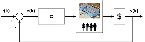
3. Development of Economic Objective Function for Advanced Building Systems Control

Considering the literature and previous works, a general component-level objective function of the form shown in Equation (1) was chosen. The quadratic terms (first and third) were included to allow for standard convex optimization when desired, where e represents the error for the system, Q the weighting placed upon the error, u the control action, and S the weighting placed on control action. The linear terms (second and fourth) were included to facilitate calculating cost purely in economic terms (dollars), as opposed to nonsensical units such as dollars squared. R and T can be formulated in such a manner to transform e and u into economic cost. This is demonstrated in subsequent sections using a specific building at Texas A&M’s campus as a case study.

$$J_{component}=e^{T}Qe+e^{T}R+u^{T}Su+u^{T}T$$

(1)

3.1. Building Configuration

For operating a typical building, there are economic costs associated with electrical cost, thermal costs, and comfort/productivity costs. The electrical costs can stem from running equipment such as electric motors in AHU fans, or from reheating air at local VAVs before it enters a zone. Thermal costs can occur from site-wide chillers that produce chilled water used to cool the air locally in buildings. Of course, comfort/productivity costs come from the thermal discomfort of the occupants. These costs exists across a wide selection of buildings/situations and can be accommodated by the general cost function above. To provide a more detailed understanding of how to derive the costs for a specific building, as well as how to construct/apply the proposed steady-state method, a case study is presented focused on a specific building, as detailed below.

Working with the Utilities Energy Management (UEM) Office at Texas A&M University, limited access was granted to the Utilities Business Office (UBO) for the purpose of collecting data and future implementation of advanced controllers. Individual component objective functions were developed for specific equipment in the UBO; however, the UBO represents a typical office building and thus the work can be generalized to other commercial buildings. What follows is a description of the UBO and its behavior to inform the development of the component objective functions.

The UBO is a rectangular, single-story building consisting of 11 zones, 10 of which are actively controlled. The general layout can be seen in Figure 2, with the thermostats shown as white boxes and the approximate locations of the VAVs shown as blue boxes. In this initial development, the decision was made to focus solely on the cooling aspects of the system because: (1) the majority of the year is spent cooling due to the location and climate of the building; and (2) simplified operating conditions will help to validate the developed control strategy in its initial implementation. The process flow and current control structure is displayed in Figure 3. The rest of this section details each of the subsystems and currently implemented controls.

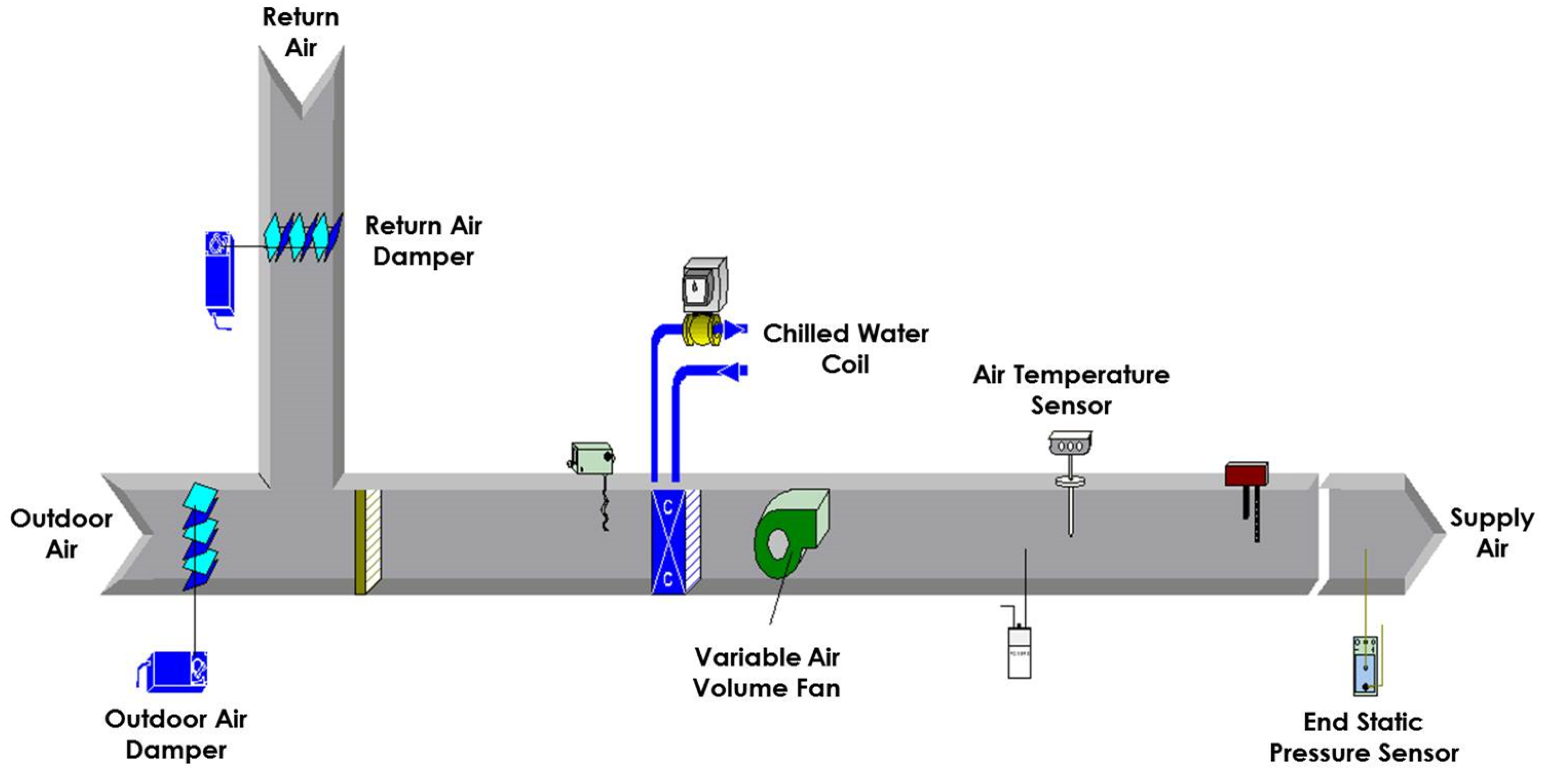
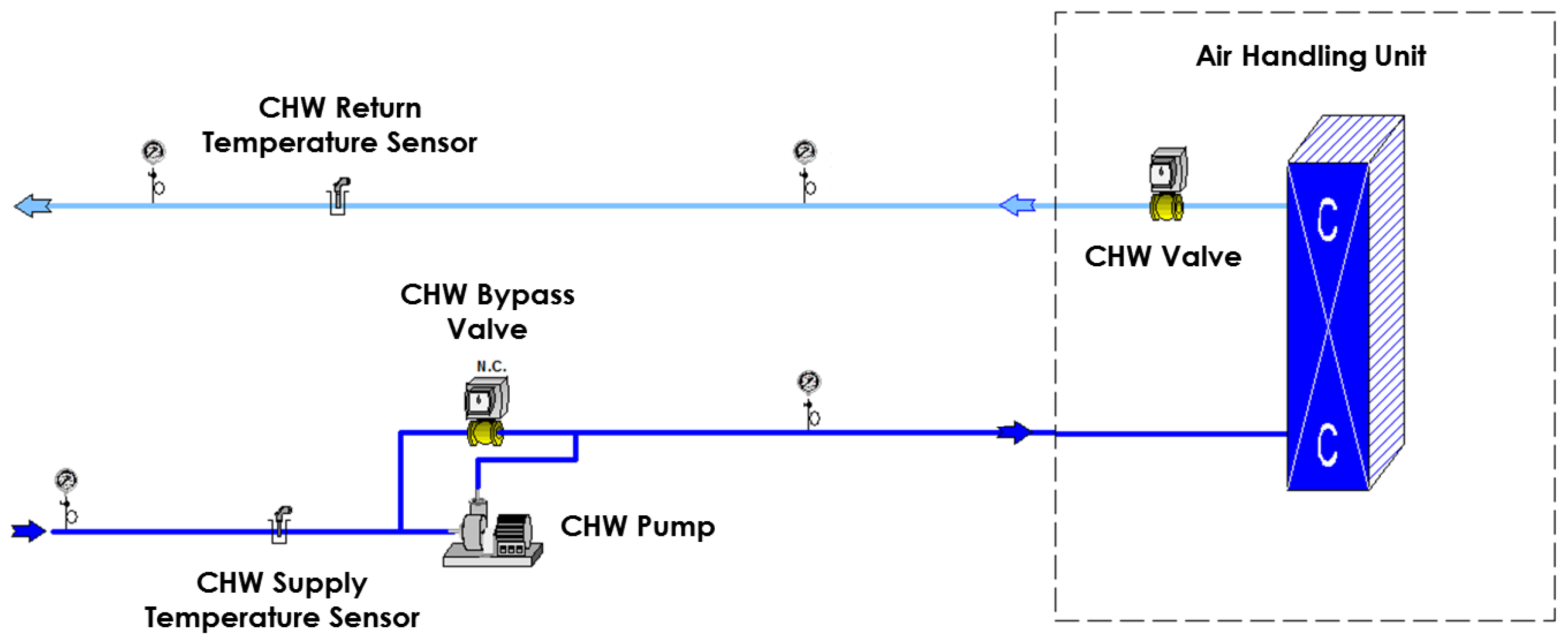
3.1.1. Rooftop Air Handling Units

Most commercial buildings are serviced by rooftop air handling units (AHUs). These AHUs serve to condition a combination of indoor air and outdoor air to meet the comfort/health requirements in one or multiple zones. In the presented case study, the UBO is serviced by a single rooftop AHU. The AHU consists of a variable air volume (VAV) fan, a chilled water coil, an outdoor air damper, a return air damper, a discharge air temperature sensor, and an end static pressure sensor. The organization of these components can be seen in Figure 4. During normal operation, the VAV fan is driven by a Proportional-Integral-Derivative (PID) loop to maintain an end static pressure setpoint given by a supervisory Proportional-Integral (PI) controller (see Figure 3 and

Table 1. Specifications for control loops in the UBO.

Controller	Reference	Feedback	Output	${\mathit{K}}_{\mathit{P}}$	${\mathit{K}}_{\mathit{I}}$	${\mathit{K}}_{\mathit{D}}$
Supervisory Controller #1	$D_{EDS}^{*}$	$D_{EDS}$	$P_{EDS}^{*}$	12	0.1	0
Fan Speed Controller	$P_{EDS}^{*}$	$P_{EDS}$	${\omega }_{fan}$	0.5	0.15	0.1
Supervisory Controller #2	$D_{CLG}^{*}$	$D_{CLG}$	$T_{DA}^{*}$	12	0.01	2000
Chilled Water Valve Controller	$T_{DA}^{*}$	$T_{DA}$	$u_{CHW}$	20	1	10
Supervisory Controller #3	Deadband Controller			N/A
Damper Controller	$T_{zone}^{*}$	$T_{zone}$	$u_{dmpr}$	Set by Manufacturer

). This PI controller’s feedback signal is a pressure demand calculation dependent upon the individual damper positions of the zone terminal boxes. This calculation is given by Equation (2).

$$D_{EDS}=\frac{1}{n}\sum _{i=1}^n{u}_{dmpr,i}·0.4+max\left(u_{dmpr,i}\right)·0.6$$

(2)

where $D_{EDS}$ is the end-static pressure demand, $n=10$ is the number of individual dampers, and $u_{dmpr}$ is the damper position. The end-static pressure demand setpoint for this supervisory PI controller stays constant at 60 (unitless) and was set during tuning by the building technicians.

3.1.2. Chilled Water Production

In many sites, chilled water is produced at a central location and used for conditioning the air in local buildings. There is a cost associated with the production of this chilled water, and it is important to capture in an economic control method. In the presented case study, chilled water provided by the central plant is passed through the UBO’s AHU chilled water coil to lower the temperature of the moving air as well as reduce the air’s humidity. The amount of chilled water passing through the coil is controlled by a valve which is actuated by a PID control loop. This control loop is driven by a difference in a discharge air temperature setpoint and the discharge air temperature. The discharge air temperature setpoint is the output of a supervisory PID control loop (see Figure 3 and Table 1) that is trying to maintain a cooling demand setpoint. A cooling demand calculation supplies the feedback signal for this supervisory controller that is a weighted combination of the average and maximum cooling loopout values from the individual zone control loops.

Figure 5 details the chilled water loop. A chilled water pump works to maintain a specific supply pressure to provide the required chilled water flow for the AHU. The chilled water supply and return temperatures are available to measure within the energy management system.

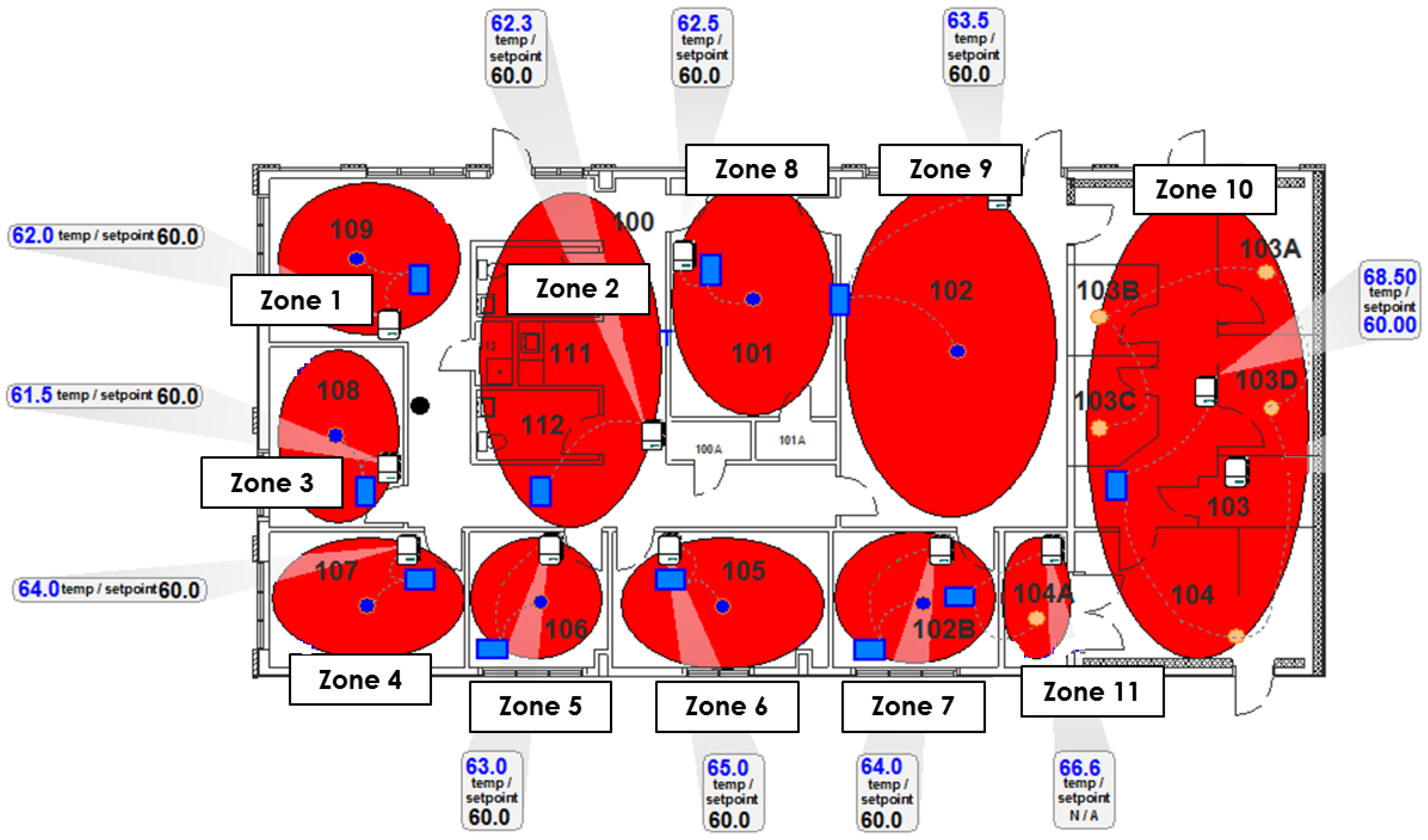
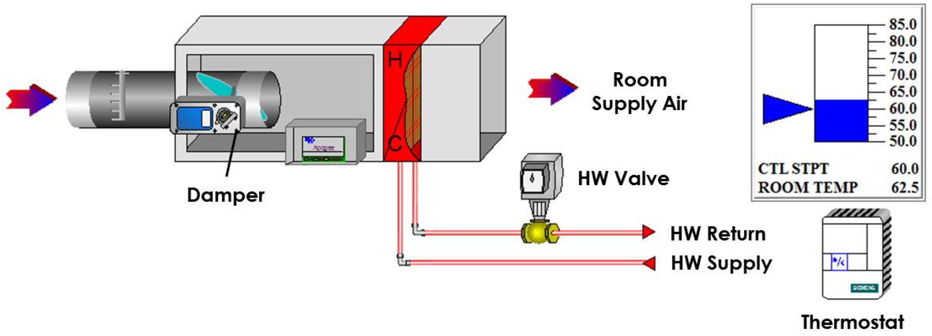
3.1.3. Conditioned Zones in Buildings

Zones within buildings can consist of one or multiple rooms, and can be serviced by one or multiple pieces of equipment. Frequently, zones in commercial buildings are assigned a VAV terminal box or damper that regulates the amount of conditioned air that is introduced to that space. There is typically a thermostat placed in the zone to provide feedback for the zone controller to regulate temperature.

As described above, the UBO consists of 11 zones, 10 of which are actively controlled. Each controllable zone is serviced by a VAV terminal box equipped with hot water reheat capabilities, an example of which is shown in Figure 6. The flow of conditioned air into the room is regulated by a damper in the terminal box whose position is determined by a PID control loop. The error signal for the control loop is the difference between the respective room temperature setpoint and the measured room temperature while the output is the damper position (see Table 1). The room temperature setpoint is determined by whether the room is occupied or unoccupied and if the zone is in heating or cooling mode. A supervisory deadband control method (see Figure 3) is employed such that if the room is occupied, the zone VAV will heat the room to 70 °F or cool the room to 74 °F. If the room is unoccupied, the VAV will heat the room to 60 °F or cool the room to 85 °F. If the occupancy sensors in all the rooms read unoccupied, then the main AHU will turn off and the room temperatures will freely fluctuate.

3.2. Economic Cost of Operating Equipment

Having described the existing equipment and controls, the following sections will outline the economic cost functions for said equipment, particularly an AHU and individual zones. Examining a typical AHU, two sources of economic cost become apparent: (1) the cost of electricity used by the AHU fan to move the air; and (2) the cost associated with the production of chilled water for cooling of the air. At the zone level, there is usually no building equipment that consumes a significant amount of power or resources (when considering cooling only applications; VAVs with local reheat would be a different situation). For example, the damper in a VAV terminal box is the only actuated component and the power required to move it is negligible.

For the presented case study, an economic objective function that minimizes the cost of occupant discomfort as a measure of the loss of productivity at the zone level was developed. As mentioned in the Background Section, select previous building energy optimizations have included some form of occupant comfort, whether simply as constraints on the optimization or as a measure to be minimized; however, to the knowledge of the authors, no previously simulated or implemented building energy optimization has considered the economic cost of occupant comfort. The following sections detail the development of these objective functions.

3.2.1. AHU Fan Economic Objective Function Development

As described above, the fan in an AHU works to maintain an end static pressure in the duct to move the required amount of air to condition the individual zones. To accomplish this, the fan motor requires electricity and there is a cost associated with the power used. A simple way to measure the power consumed by a fan motor would be to use a power meter on the electrical lines to the fan and measure the power consumed; however, power meters are not often included on individual fans within existing building energy systems. Therefore, for the presented case study of the UBO, the power consumed by the fan was instead determined by other available data. Specifically, the change in pressure across the fan and the volume flow rate of air were used. With these two values, the work being performed by the fan on the air can be estimated and converted into a measure of power. The equation for work performed by a fan is given in Equation (3):

$$P_{fan}=0.1175·\frac{q_{AHU}·\Delta P}{{\mu }_f·{\mu }_b·{\mu }_m}$$

(3)

where $P_{fan}$ is the power consumed by the fan [W], $0.1175$ is a conversion factor for imperial units, $q_{AHU}$ is the air flow rate through the AHU [cfm], $\Delta P$ is the change in pressure across the fan [in. ${\mathrm{H}}_2\mathrm{O}$], and ${\mu }_f,{\mu }_b,\mathrm{and}{\mu }_m$ are efficiencies for the fan blade, the fan belt, and the fan motor, respectively. The efficiencies were all assumed to be 0.9 based on comparable values to reflect some degradation from the ideal efficiencies of new/perfectly tuned equipment. The change in pressure across the fan was taken from the end static pressure sensor in the AHU. As for the volume flow rate, the flow rate meters included in each of the VAVs were used in summation to calculate the total air flow rate through the AHU, assuming minimal duct losses and leaks.

The most appropriate control action u for the AHU fan objective function would be the end static pressure setpoint. Assuming the local PID controllers have zero steady state error and sample significantly faster than the new supervisory controller, a reasonable assumption can be made that the end static pressure will equal the end static pressure setpoint. As such, assuming an electric utility rate of $0.12 per kWh, the fan power cost can be calculated as:

$$J_{fan}=\frac{0.1175}{1000}·\frac{C_{elec}·q_{AHU}·P_{EDS}^{*}·t_s}{{\mu }_f·{\mu }_b·{\mu }_m}$$

(4)

where $C_{elec}$ is the rate of electricity cost [$/kWh], $P_{EDS}^{*}$ [in. H${}_2$O] is the end static pressure setpoint, and $t_s$ [hr] is the sampling time of the supervisory controller. Reformulating Equation (4) to fit Equation (1) gives:

$$\begin{array}{c}{J}_{fan}=e^{T}Qe+e^{T}R+u^{T}Su+u^{T}T\\ Q=0R=0S=0\\ u=P_{EDS}^{*}\\ T=\frac{0.1175·C_{elec}·q_{AHU}·t_s}{1000·{\mu }_f·{\mu }_b·{\mu }_m},\end{array}$$

(5)

thus establishing an objective function that can minimize the cost of electricity used by the AHU’s VAV fan by optimizing the end static pressure setpoint.

3.2.2. AHU Chilled Water Economic Objective Function Development

As described in the building operation details, chilled water is used in the AHU to condition the zone supply air. If specific details about the chiller are known, the consumption of power can be calculated and then used to determine the cost of producing said chilled water. In the case study, utility usage data were leveraged to determine this cost. The UEM Office at Texas A&M University maintains utility usage data, specifically the cost per unit of energy of the respective utility. For chilled water, this is the dollar cost associated with producing one mmBtu of chilled water at the campus wide chilled water temperature of 45 °F. In the AHU, the discharge air temperature setpoint is tracked by a PID loop that actuates the valve metering how much chilled water flows through the chilled water coil. The energy associated with chilled water usage can be determined by Equation (6):

$$\dot{Q}=\dot{m}·c·\Delta T$$

(6)

where $\dot{Q}$ is the rate of change of heat, or energy, $\dot{m}$ is the mass flow rate, c is the specific heat of the respective fluid, and $\Delta T$ is the change in temperature of the fluid. If a mass flow rate sensor is available on the AHU for the chilled water, then this measurement can be used to calculate the rate of change of energy of the chilled water and thus the overall cost; however, mass flow rate sensors are not usually installed on chilled water lines at the AHU level. If this is the case, then a volume flow rate can be used such that:

$$\dot{m}=\rho ·q$$

(7)

where $\rho$ is the density of water and q is the volume flow rate. With the UBO, the maximum flow rate through the chilled water valve was determined to be $3.41e^{-3}$${\mathrm{m}}^3/\mathrm{s}$ (54.05 gal/min). Assuming a linear valve/flow relationship, the chilled water valve position multiplied by the maximum possible flow will give the current volume flow rate of the chilled water. Using data values for the discharge air temperature setpoint and the chilled water valve position, a fit was generated to transform the setpoint to a valve position [31]. Combining the relationships gives Equation (8)

$$\begin{array}{c}{J}_{CHW}=\alpha ·q_{max}·\rho ·c·\Delta T_{h_{2}o}·t_s·0.00341214·\frac{3682}{241}\\ \alpha =\left(3.021T_{DA}^{*2}-109.4T_{DA}^{*}+1002\right)\end{array}$$

(8)

where $\alpha$ is the fitted relationship between the discharge air temperature setpoint ($T_{DA}^{*}$ [${}^{\circ }$C]) and the chilled water valve position [%], $q_{max}$ [${\mathrm{m}}^3/\mathrm{s}$] is the maximum flow through the valve (at 100% opening), $\rho$ [kg/m${}^3$] is the density of water, c [kJ/kg ${}^{\circ }$C] is the specific heat of water, $\Delta T_{h_{2}o}$ [${}^{\circ }$C] is the change in temperature of the supply and return chilled water, $t_s$ [h] is the sample time of the supervisory controller, $0.00341214$ [mmBtu/kWh] is a conversion factor from kWh to mmBtu, and the last term is the economic cost for the UBO of the consumed chilled water. Reformulating Equation (8) to fit Equation (1), where u equals the discharge air temperature setpoint, gives:

$$\begin{array}{c}{J}_{CHW}=e^{T}Qe+e^{T}R+u^{T}Su+u^{T}T\\ Q=0R=0S=0\\ u=\alpha =\left(3.021·T_{DA}^{*2}-109.4·T_{DA}^{*}+1002\right)\\ T=q_{max}·\rho ·c·\Delta T_{h_{2}o}·t_s·0.00341214·\frac{3682}{241}\end{array}$$

(9)

where the linear cost term $u^{T}T$ is equal to Equation (8). This result actually lends itself well to traditional convex optimization of the setpoint $T_{DA}^{*}$, due to the quadratic nature of the fit.

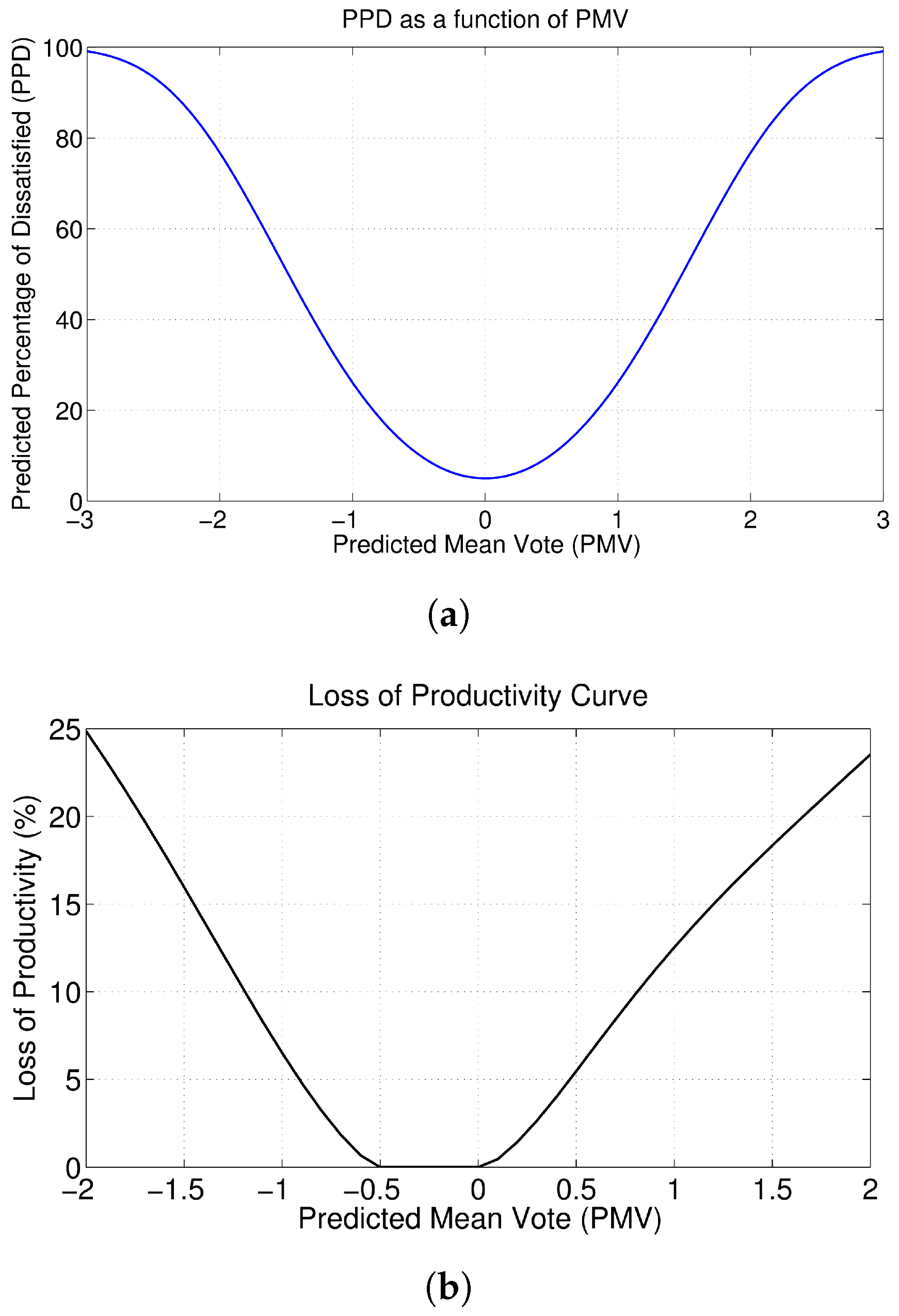
3.2.3. Zone Occupant Comfort Economic Objective Function Development

To measure an occupants level of discomfort, many have relied on the use of predicted mean vote (PMV), developed by Fanger in the 1970s [29]. PMV is a measure on the American Society of Heating, Refrigeration, and Air-Conditioning Engineers (ASHRAE) thermal sensation scale of −3 to 3, where negative numbers represent being too cold, positive numbers represents being too warm, and a value of zero represents being comfortable. Performing a large study of people, Fanger collected data regarding occupants votes and created an equation to determine the PMV across a variety of environmental factors. These factors include air temperature, air relative humidity, relative air speed, mean radiant temperature, an occupant’s insulation level due to clothing, an occupant’s metabolic rate, and an occupant’s work output, among several other variables. The details of the equation can be found in [29]. From PMV, Fanger determined the Predicted Percentage of Dissatisfied (PPD) of people. The relationship of PPD to PMV can be seen in Figure 7a.

One can see that at −3 and 3 PMV approximately 100% of the population would be dissatisfied. Of note is that, even at 0 PMV, 5% of the population, on average, will still be dissatisfied, attesting to the fact that each individual has specific preferences. While PMV determines how many people will be dissatisfied, a relationship to tie this to an economic cost is still needed.

Fortunately, researchers have investigated the effect of occupant comfort on worker productivity, as mentioned in the literature review. One effort in particular tied PMV to a measure of Loss of Productivity (LOP) [%]. By using regression analysis, a direct relation can be calculated between a worker’s loss of performance and the PMV of an indoor climate by including the calculations of equivalent thermal situations from Gagge’s two-layer human model [33] and Fanger’s comfort equation [29]. For a detailed explanation of the relationship, see [32]. The results of Roelofsen’s work [32] are two sets of coefficients for a regression fit for the cold side of the PMV comfort zone and for the warm side of the PMV comfort zone. The regression is the sixth-order fit shown in Equation (10):

$$\begin{array}{c}LOP=c_0+c_{1}PMV+c_{2}PM{V}^2+c_{3}PM{V}^3+c_{4}PM{V}^4+c_{5}PM{V}^5+c_{6}PM{V}^6\end{array}$$

(10)

where $LOP$ is the loss of productivity and $c_0,\dots ,c_6$ are the regression coefficients. The value of the Roelofsen’s coefficients are repeated in

Table 2. Regressions for loss of productivity fit of PMV; values presented in [32].

Regression	Cold Side of	Warm Side of
Coefficients	PMV Comfort Zone	PMV Comfort Zone
$c_0$	1.2802070	−0.15397397
$c_1$	15.995451	3.8820297
$c_2$	31.507402	25.176447
$c_3$	11.754937	−26.641366
$c_4$	1.4737526	13.110120
$c_5$	0.0000000	−3.1296854
$c_6$	0.0000000	0.29260920

, for reference. Roelofsen constructed the regression on the cold side to be zero at −0.5 PMV and for the warm side to be zero at 0 PMV, leaving a region between −0.5 and 0 PMV where LOP is zero. This bias is because several studies found a region of conditions near and below 0 PMV that had a negligible effect on productivity. Figure 7b shows the change in LOP as PMV varies.

To connect LOP to an economic cost, a multiplication of the lost productivity percentage by the amount of salary an employee earns over the sample period can be used, as shown in Equation (11):

$$\beta =LOP·\left(\frac{p_{year}·t_s}{52·40}\right)$$

(11)

where $\beta$ [$] is the lost productivity in wages, $p_{year}$ [$] is the annual salary for the zone, and $t_s$ [h] is the sampling time. A 40-h work week for the entire year was used as a conservative assumption. In reality, there will be some variation due to holidays, vacation, and overtime.

Considering the individual zones in the presented case study with respect to Equation (1), it is noted that, while there is no control action u at the zone level that consumes energy, there is an error signal present. That is the error e in Equation (1), which is given by:

$$\begin{array}{c}e=T_{zone}-T_{zone}^{*}\end{array}$$

(12)

where $T_{zone}$ and $T_{zone}^{*}$ are the zone temperature and zone temperature setpoint, respectively. The error is defined in this manner as this publication focuses on the systems when in cooling mode; thus, the error will be mostly positive during cooling mode. If the zone were in heating mode, the sign of the error term would need to reversed. Recognizing that the zone temperature setpoint can be optimized by the supervisory controller to minimize the LOP by optimizing the zone’s PMV, and that the error signal is a difference of temperatures, the sensitivities of the above relationships can be determined and combined to give an economic objective function.

In determining PMV, only the zone air temperature and zone air relative humidity are changing. As such, a fit of the PMV equation was created and used to reduce computation time and complexity. A metabolic rate of 70 [W/m${}^2$], a clothing insulation factor of 0.75 [m${}^2$K/W], and a relative air velocity of 0.2 [m/s] were assumed. Additionally, the mean radiant temperature was assumed to be equal to the zone air temperature. The fit is defined as:

$$\begin{array}{c}PMV=0.5542·R{h}_{zone}+0.23·T_{zone}-5.44\end{array}$$

(13)

where $R{h}_{zone}$ [%] is the relative humidity of the zone and $T_{zone}$ [${}^{\circ }$C] is the zone air temperature. Equation (13) is used to determine the sensitivity of PMV to changes in air temperature. The resulting combination of sensitivities is shown in Equation (14):

$$\begin{array}{c}{J}_{room}=e^{T}Qe+e^{T}R+u^{T}Su+u^{T}T\\ Q=0S=0T=0\\ R=\left[\frac{\partial PMV}{\partial T_a}\right]·\left[\frac{\partial LOP}{\partial PMV}\right]·\left[\frac{\partial \beta }{\partial LOP}\right]\end{array}$$

(14)

where the sensitivities are determined to be:

$$\begin{array}{c}\left[\frac{\partial PMV}{\partial T_a}\right]=0.23\end{array}$$

(15)

$$\left[\frac{\partial LOP}{\partial PMV}\right]=c_1+2c_{2}PMV+3c_{3}PM{V}^2+4c_{4}PM{V}^3+5c_{5}PM{V}^4+6c_{6}PM{V}^5$$

(16)

$$\begin{array}{c}\left[\frac{\partial \beta }{\partial LOP}\right]=\left(\frac{p_{year}·t_s}{52\mathrm{wks}·40\mathrm{hrs}}\right).\end{array}$$

(17)

The cost calculation assumes that, if more than one occupant is in a zone, the sum of the occupant’s salaries is used for $p_{year}$. For Equation (16), the coefficients are as described in Table 2. If the zone’s PMV falls within the range of −0.5 to 0, then Equation (16) is equal to zero. The overall trend of the objective function as the zone air temperature varies is shown in Figure 8. The abrupt changes occur at the PMV values of −0.5 and 0, due to the fit of the LOP equation.

This curve will shift depending on other variables in the objective function that are varied, such as annual salary and relative humidity of the zone. In addition, depending on the value of the user-defined setpoint, the objective cost can become negative. This does not mean that the zone is earning money, but occurs because of the structure of the objective function. An optimization competition can occur between the error term and the coefficient R. As the error is defined as the difference in the zone temperature and zone temperature setpoint, the objective cost will be zero when the zone reaches this defined setpoint; however, if this setpoint is not equal to the optimal comfort temperature, as determined by the PMV function, then the objective cost will also be zero if the zone air temperature is equal to the optimal comfort temperature.

This behavior presents an interesting control question. To operate at the most cost effective point, as defined by the objective function, would require that the zone temperature setpoint be set to the PMV optimal temperature, but, in doing so, the ability for occupants or building managers to provide the system feedback about their comfort is removed. Thus, which is more important: the ability for occupants to choose their zone temperatures or allowing the system to determine what is best for the occupants? This question deserves additional investigation but is beyond the scope of this publication. Fortunately, with this objective function, the system will propose a compromise: a temperature between the user-defined setpoint and the PMV optimal comfort temperature.

For a centralized implementation, the objective function then becomes:

$$\begin{array}{c}{J}_{total}=J_{fan}+J_{CHW}+{\displaystyle \sum _{i=1}^n}{J}_{zone,i}\end{array}$$

(18)

where n is the number of zones in the system. Equation (18) is the system objective function that will be minimized in the optimization.

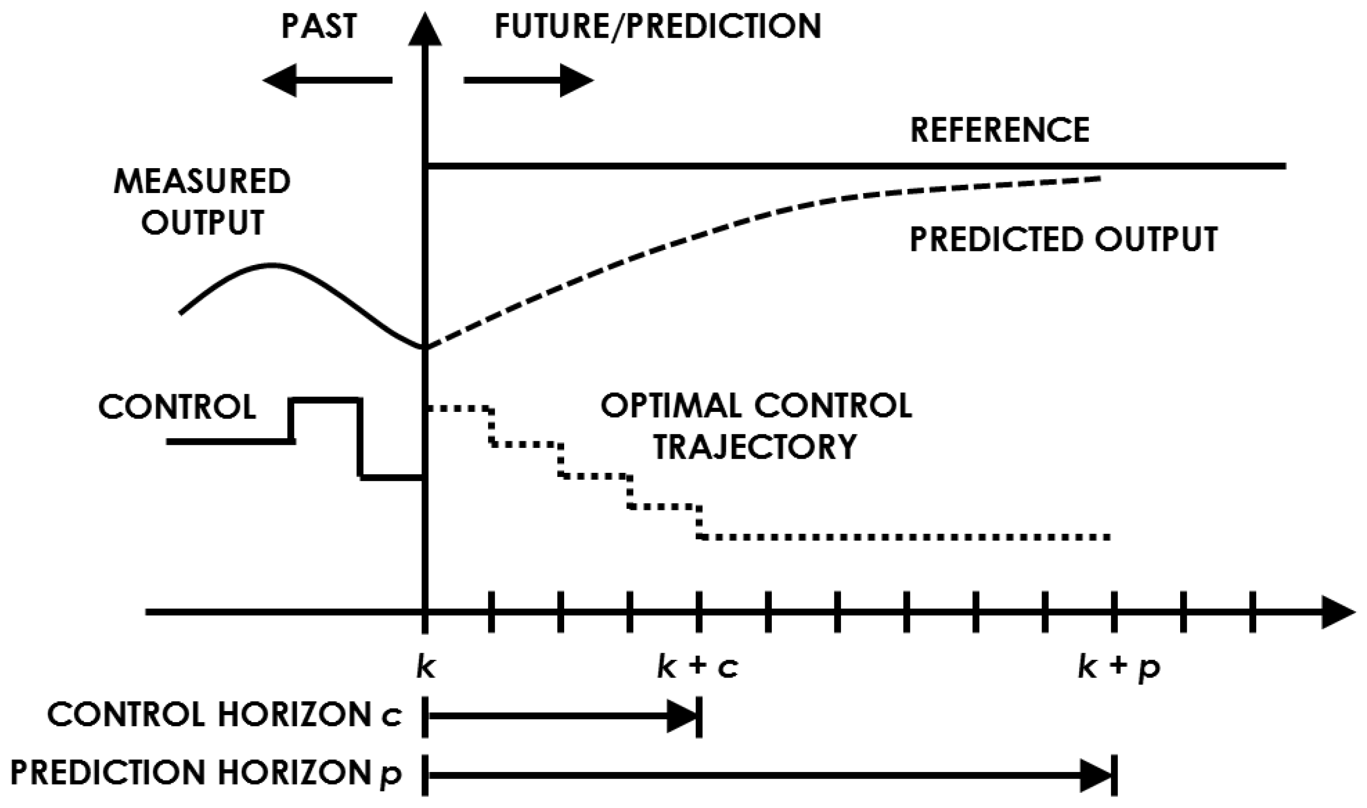
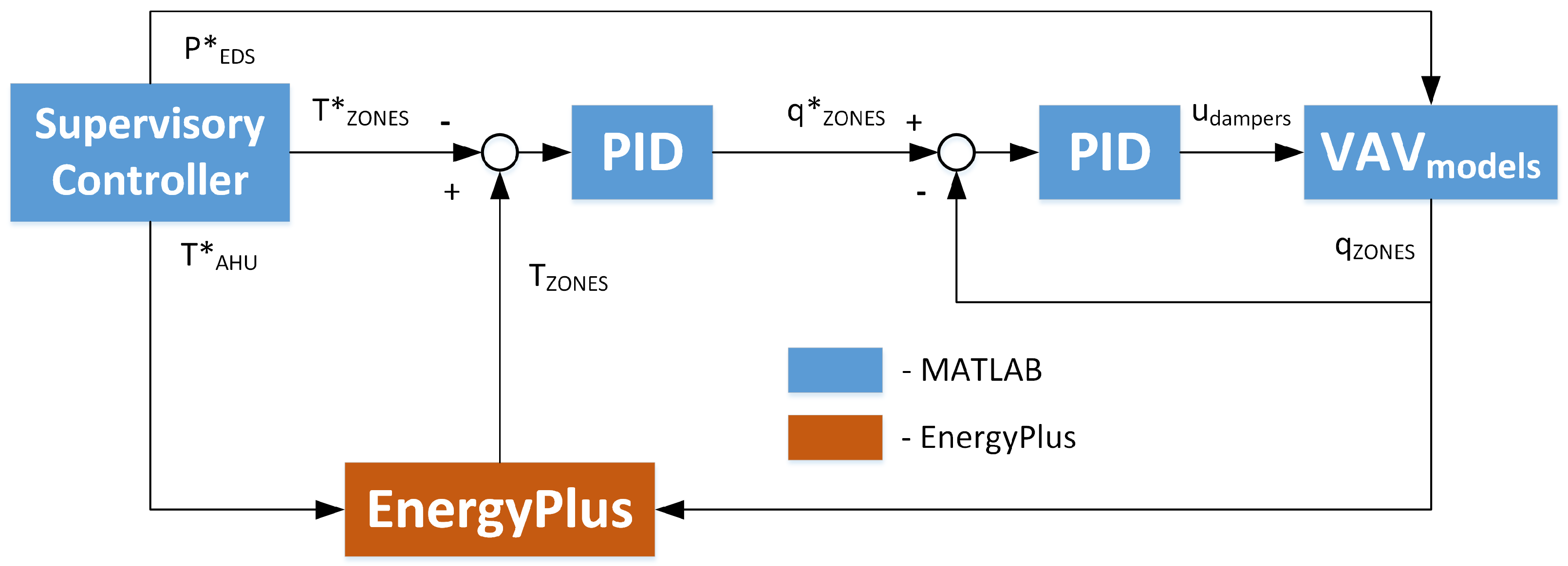
4. Simulation Design

A model of the UBO was first created with the aid of SketchUp [34], a 3D modeling software. Using dimensions taken from the building, the single story layout was replicated. Utilizing the plug-in from OpenStudio, thermal zones, boundaries, and interactions were defined. This model was then exported as an input file (IDF) for EnergyPlus [35], an open-source energy simulation program that has been developed by the Building Technologies Office (BTO) under the U.S. Department of Energy (DOE). Using EnergyPlus, HVAC equipment was added to the model based on the equipment present in the UBO. While EnergyPlus excels at modeling and simulation, it is not immediately accessible for controller development and implementation. As such, controllers for the AHU and the zone level VAVs were created in MATLAB. To enable co-simulation between EnergyPlus and MATLAB, two programs were used. The first was MLE+ [36], an open-source MATLAB toolbox for creating the necessary configuration files and providing functions to connect EnergyPlus and MATLAB with an easy-to-use graphical interface. MLE+ utilizes the Building Controls Virtual Test Bed (BCVTB) [37] as the communication backend between EnergyPlus and MATLAB, providing the co-simulation functionality.

The individual zones of the model were setup as defined in the building layout and exterior doors and windows were placed as accurately as possible. The AHU and zone VAVs were added using EnergyPlus’ HVACTemplate objects. A central electric chiller was also added to supply chilled water to the AHU. The chilled water output temperature is regulated to 45 °F, the same as the supply chilled water temperature for the UBO.

Currently, EnergyPlus does not offer modeling of pressure with variable air volume systems, thus another solution was necessary to simulate the UBO’s control and physical limitations of end static pressure and flow in the AHU. To accomplish this, the authors assumed that the dynamics of the fan speed and end static pressure were fast enough compared to the simulation timestep (1 min) to be considered instantaneous. Additionally, the assumption that the fan would supply the requested end static pressure, constrained by the physical limitations of the AHU and ducting, was made. To determine this constraint, data from the real UBO building were analyzed and a maximum possible work performed by the fan was calculated (910 W). During the optimizations, the constraint is calculated by using Equation (19).

To determine the total volume flow through the AHU, individual models of the zone VAVs were generated from data based on VAV damper position and end static pressure. The effect of outdoor air temperature was also considered on the VAVs as the AHU draws in outdoor air, but was shown to be minimal. This is most likely due to the fact that AHU is able to meet its discharge air temperature setpoint, even at varying flows, effectively isolating the VAV supply air from the outdoor air conditions. The flows from the VAV models are summed to obtain the total flow through the AHU, assuming minimal duct losses. The constraint can be written as:

$$910\ge 0.1175·\frac{q_{AHU}·P_{EDS}}{{\mu }_f·{\mu }_b·{\mu }_m}$$

(19)

Thus, the optimization will only ever choose an end static pressure setpoint that is physically achievable by the system. This end static pressure is then passed to the VAV models which, along with the commanded damper positions, produce individual zone air volume flows.

The overall control hierarchy can be seen in Figure 9. The supervisory controller supplies the zone temperature setpoints ($T_{ZONES}^{*}$) to the respective PID reference inputs and the end static pressure setpoint ($P_{EDS}^{*}$) to the VAV models. The discharge air temperature setpoint ($T_{AHU}^{*}$) is supplied directly to EnergyPlus as the control for the chilled water valve is implemented using an appropriate setpoint manager within EnergyPlus. The zone temperature error is fed to the cooling PID controller which outputs a desired percentage of maximum flow setting (0–100%). If the minimum flow setting for a zone is zero, then the signal remains unchanged. The desired flow percentage is then passed to the flow PID controller which then produces a desired damper position. This damper position is used in the VAV models as previously described. The outputs from the VAV models, desired zone air volume flows, are converted to air flow fractions and then sent to zone VAVs in EnergyPlus where the room dynamics are simulated for one timestep.

For the supervisory controllers, a prediction model is necessary to determine the future zone temperatures as the setpoints are optimized. A previously developed modeling algorithm was employed to generate models for the individual zones [38]. One of the main reasons this algorithm was chosen is because of its ease in producing models, requiring the user to only select input and output data. The full details of this process are beyond the scope of this publication, but more information can be found in [38]. Briefly, data from the EnergyPlus simulation are analyzed to develop discrete, linear models of the selected parameters. These models take the form of:

$$\begin{array}{c}{x}_i(k+1)=A_i{x}_i\left(k\right)+B_i{u}_i\left(k\right)+K_i{e}_i\left(k\right)\\ y_i\left(k\right)=C_i{x}_i\left(k\right)\end{array}$$

(20)

where A, B, C, and K are the identified system matrices, u is the model input vector, y is the predicted output, and e is the error defined as the difference between the current value and the previous predicted value. The algorithm automatically identifies significant coupling interactions between zones and includes the respective zone temperatures ($T_{zonedist.,j}$) as measured disturbances. In addition to the temperature of these disturbance zones, other parameters such as outdoor air temperature ($T_{OA}$), outdoor air relative humidity ($R{h}_{OA}$), AHU discharge air temperature ($T_{AHU}$), end static pressure ($P_{EDS}$), and zone temperature setpoints ($T_{zone,i}^{*}$) are used as inputs to ARX, ARMAX, Output Error, and Box-Jenkins modeling methods with the output being the respective zone temperatures ($T_{zone,i}$). The best fitting model is selected and then the individual models are combined into a centralized model of the entire system. Steady-state predictions from this centralized model are then used by the supervisory controller to optimize the UBO’s 12 setpoints (discharge air temperature setpoint, end static pressure setpoint, and 10 zone temperature setpoints) to minimize the economic cost functions previously described. The optimization occurs every 15 min with the R, S, and T matrices updating based on current operating conditions to reflect the time varying nature of the system dynamics.

Steady-state relationships were chosen over dynamic relationships for the initial implementation and validation of the proposed economic objective function strategy. This choice takes advantage of the fact that in the building energy systems, the control variable’s dynamics (AHU discharge air temperature, end static pressure, VAV damper position) change quickly versus the other system variables (outdoor air temperature, outdoor relative humidity, room temperature), which change relatively slowly over the optimized timestep. The exact model inputs and outputs are shown in

Table 3. Inputs and outputs for the generated zone models.

Model Input	Model Output
$T_{OA}$
$R{h}_{OA}$
$T_{zone,i}^{*}$	$T_{zone,i}$
$T_{AHU}^{*}$
$P_{EDS}^{*}$
$T_{zonedist.,j}-T_{zone,i}$

.

Models were identified for two operational cases: (1) where the zone VAV damper still had actuator range (i.e. the damper was not fully open); and (2) where the zone VAV damper is fully open. The separate models were necessary as the effect of the model inputs varies greatly between the two cases. In Case 1, the effect of $T_{AHU}^{*}$ and $P_{EDS}^{*}$ are minimal compared to $T_{zone,i}^{*}$. This is due to the fact that the VAV damper is actuated by a PID controller with $T_{zone,i}^{*}$ as the reference. The PID controller is able to reject changes in $T_{AHU}^{*}$ and $P_{EDS}^{*}$ by changing the damper position to achieve $T_{zone,i}^{*}$. However, in Case 2, when the damper is fully open, $T_{AHU}^{*}$ and $P_{EDS}^{*}$ become the inputs of significance as they directly effect the zone temperature, determining the amount and the temperature of the incoming conditioned air.

A decision process was necessary to determine when each model should be used. This decision was made based off of two conditions. The first determined if the predicted zone temperature using the Case 1 models was greater than the prediction from the Case 2 models. This condition served to verify whether the predicted temperature from the Case 1 models was currently achievable with the state of the AHU. If the Case 1 predicted temperature was lower than the Case 2 predicted temperature, then the VAV would not be able to achieve the Case 1 predicted temperature with the current $T_{AHU}^{*}$ and $P_{EDS}^{*}$ values. The second checked if the current VAV damper position was less than 95%, or, in other words, if the VAV still had actuator range of the damper. The value of 95% was used as opposed to 100% to serve as a threshold and help prevent the system from oscillating between cases. If both these conditions were true, then the Case 1 models were used; otherwise, the Case 2 models were used. To help ensure smooth transfer between the two models and more accurate predictions, errors were calculated between the previous predictions the measured temperatures and included in the current prediction.

5. Results

Simulations were completed to determine the steady-state optimal control method’s performance compared to the current control strategies in place in the UBO, using Equation (18) as the objective function. An additional simulation was completed to demonstrate the current control method’s ability to track LOP optimal (PMV = −0.25) zone temperature setpoints. By using LOP optimal temperature setpoints, a more direct performance difference can be determined between the current control method and the proposed steady-state optimal control method. Lastly, a simulation showcasing the proposed optimal control method’s ability to prioritize certain zones over other zones was completed.

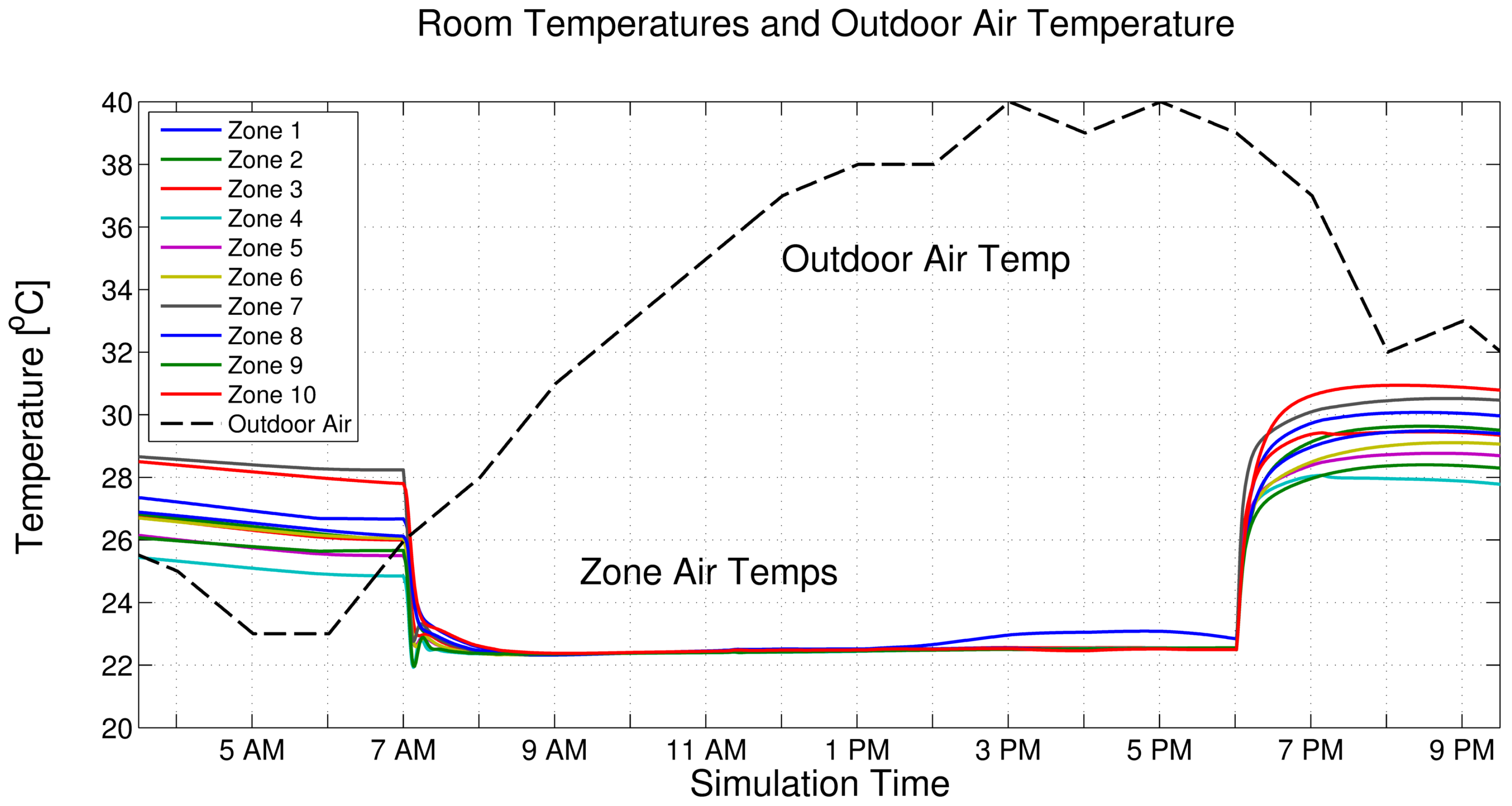
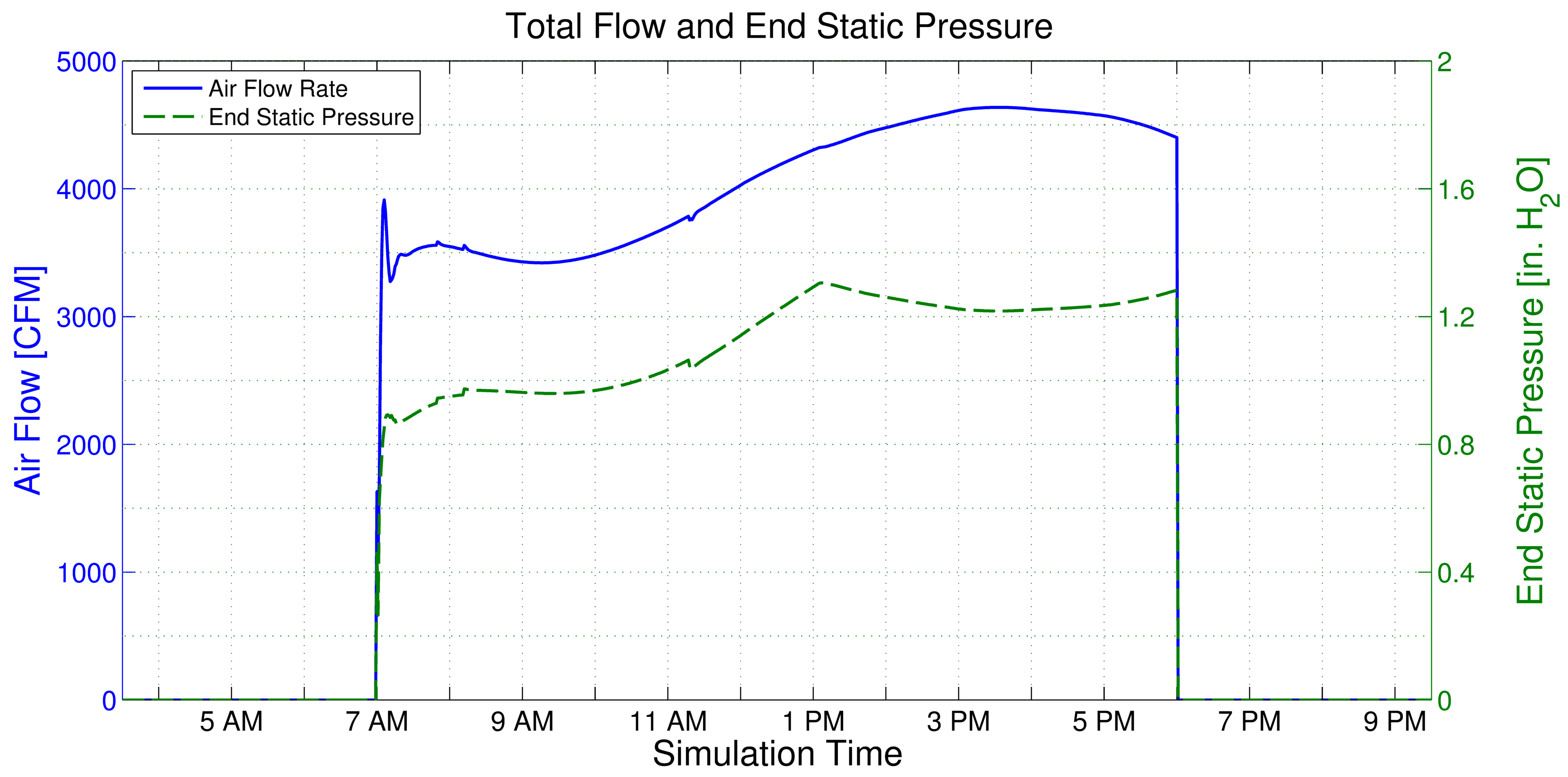
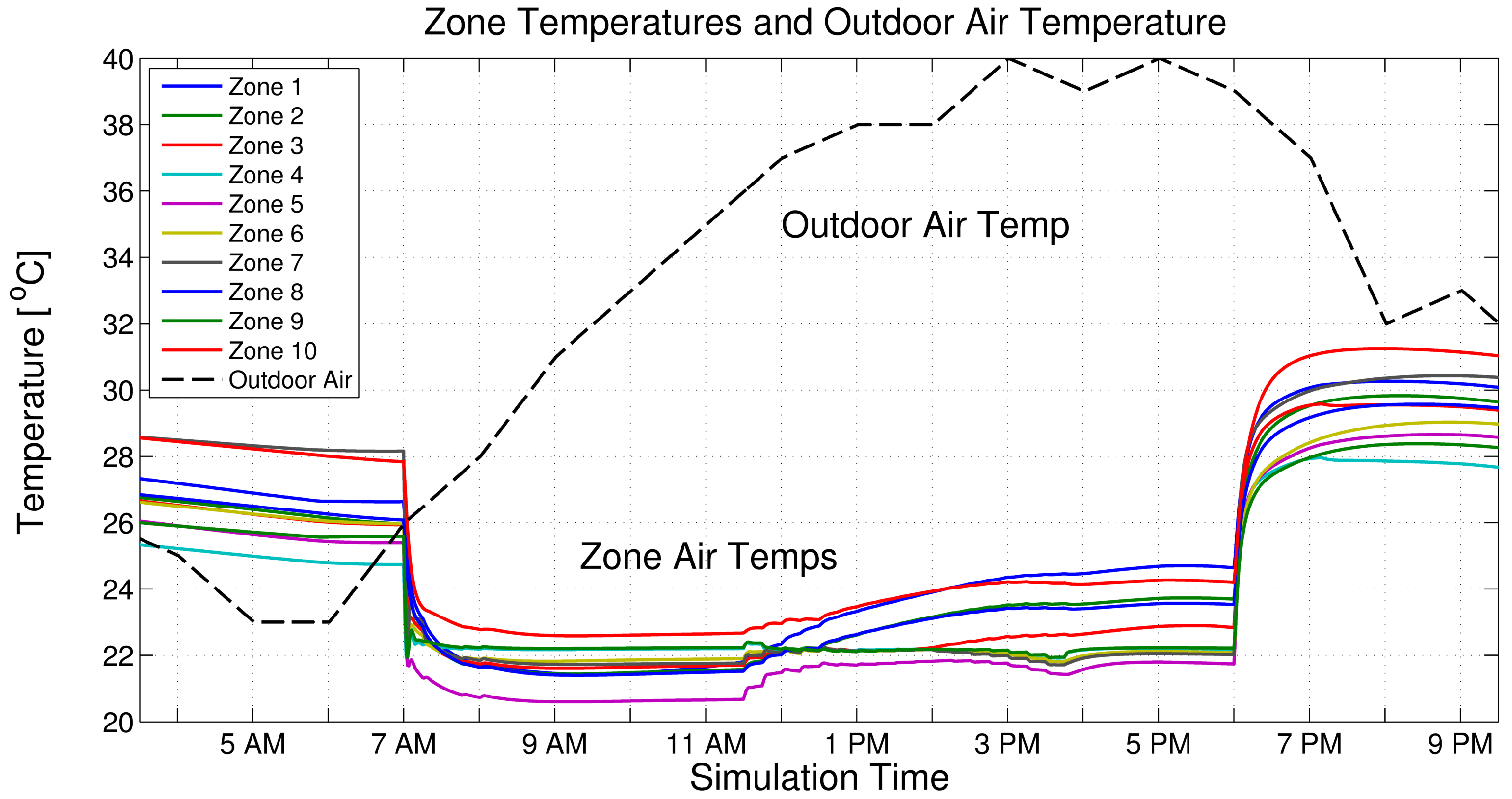
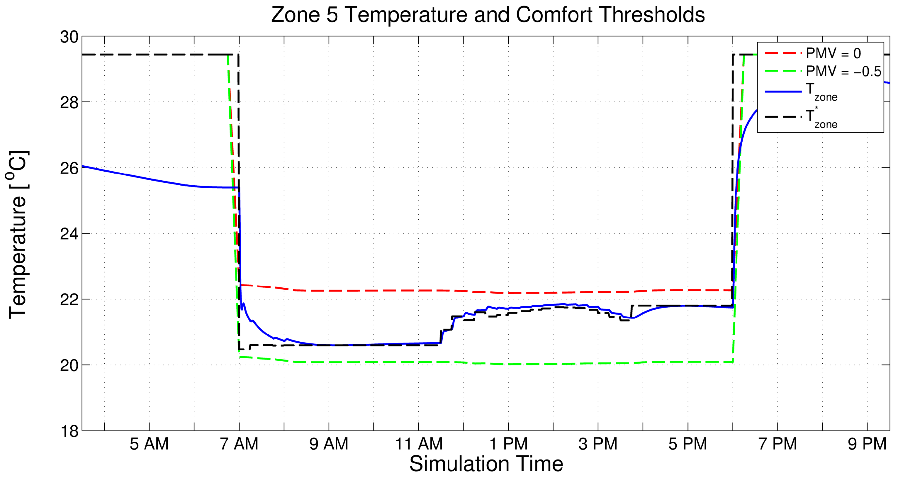
5.1. UBO Simulation with Current Building Controls

The current control method was simulated on the UBO building under two operational cases: (1) with the building operator defined zone temperature setpoints (23 °C); and (2) with LOP optimal zone temperature setpoints (the air temperature at which PMV = −0.25). The numerical results of the first case are used as a baseline to compare against, while this section details the performance of the second case. Figure 10 shows one day of the zone temperatures for the UBO building using the current control method and PMV optimal temperature setpoints. The outdoor air temperature (dashed line) is included in the plot for reference.

The current control method with demand calculations and local PID control shows the ability to track the LOP setpoints fairly accurately. Worth noting is that beginning around 2 pm, Zone 1’s temperature starts to drift upwards away from the optimal temperature. This is due to Zone 1’s damper being fully open combined with the fact that the AHU fan has reached its power limit and the discharge air temperature is not decreasing fast enough to provide the additional required cooling. Figure 11 shows the system’s end static pressure (dashed green line) and the total air flow (solid blue line) in the AHU. Shortly after 1 PM, the end static pressure begins to decrease as the total air flow continues to increase. This is the point where the AHU fan has reached its maximum power capabilities. As the zone dampers continue to open, there is less obstruction to the passage of air, decreasing the pressure and increasing the flow.

Figure 12 shows the chilled water flow and discharge air temperature of the AHU. The discharge air temperature gradually decreases throughout the day (dashed green line), responding to the increase in cooling demand. As the temperature drops, more chilled water is required to cool the air, displayed by the increase in the mass flow rate of the chilled water (solid blue line).

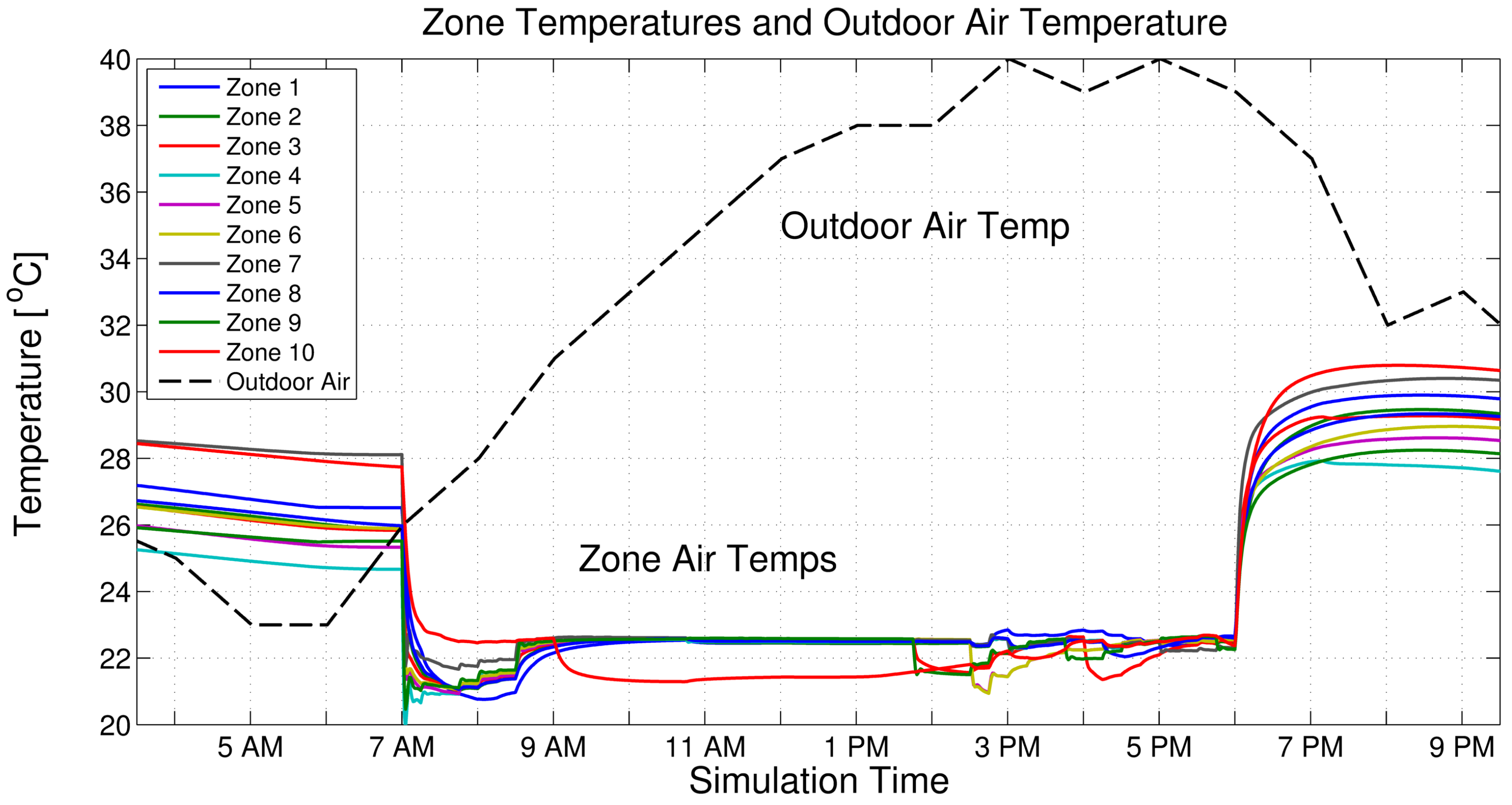
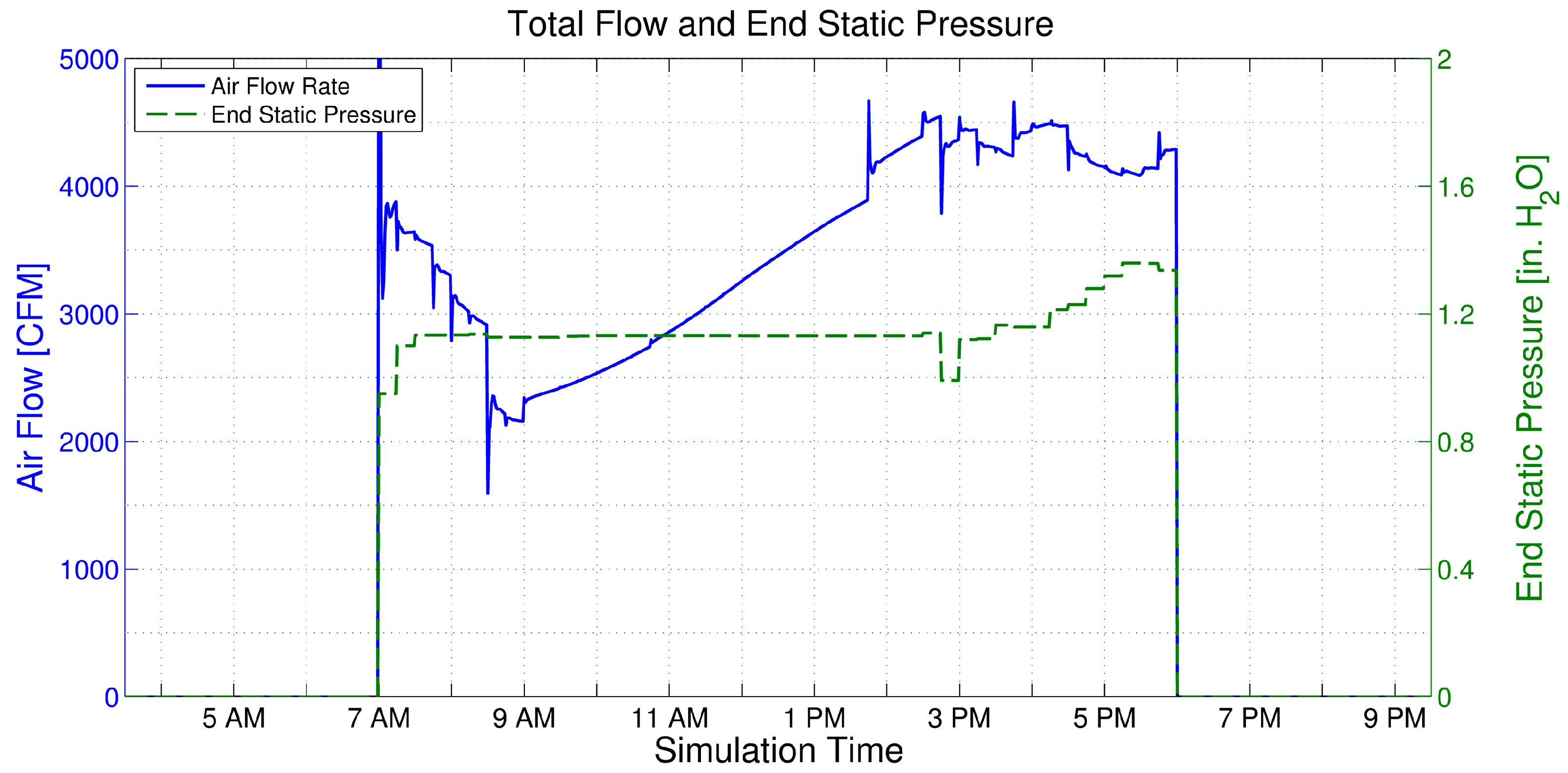
5.2. Steady-State Optimal Control Simulation

The proposed steady-state optimal control method was simulated on the UBO building with the user-defined temperature setpoints equal to the PMV optimal temperature. All the zone temperatures can be seen in Figure 13. Compared to Figure 10, the zone temperatures appear to vary slightly more through out the day. This is not because the zones temperatures are not optimal, but because of the range of PMV (−0.5 to 0) for zero loss of productivity. This range of PMV’s allows the optimization a band in the individual zone temperatures while minimizing the utility cost of the chilled water and electricity and leveraging the coupling that exists between zones.

Figure 14 shows the end static pressure and the total air flow through the AHU. Comparing to the current control method simulation, the air flows follow relatively similar paths, with the pressure in the steady-state method simulation taking a higher value but remaining more constant throughout the day. Figure 15 shows a lower discharge air temperature for the steady-state case. While this results in increased flow rates of the chilled water, the cost may not necessarily be higher as the return chilled water temperature may be lower, meaning the chiller has to cool the water over a smaller difference in temperatures. This lower discharge air temperature helps the steady-state optimal control method to achieve more reduction in the cost of lost productivity due to discomfort, enabling lower temperatures in the zones.

5.3. Very Important Person Simulation

To demonstrate one of the proposed steady-state algorithms capabilities, a simulation in which the comfort conditions of one zone was valued significantly more over the other zones in the building was completed. This can occur in the situation where there is a very important person (VIP) that requires comfortable conditions to be maintained, or in the case where other rooms are less important to maintain at a specific comfort level and can be warmer to reduce utility usage. In this simulation, Zone 5 was chosen as the VIP zone. Figure 16 shows all of the zone temperatures. The other zones are higher in temperature throughout the day, while Zone 5 is maintained at a lower temperature. Several zone temperatures can be seen rising above the 0 PMV threshold after 1 PM, when the cooling demand for the day is the greatest. This departure from the optimal LOP range between −0.5 and 0 PMV is due to the optimization balancing the cost of discomfort in the zones with the cost of the utilities.

Figure 17 provides further insight into the maintaining of comfort in Zone 5. The zone temperature is shown with the solid blue line and two thresholds are displayed: (1) the dashed red represents the 0 PMV threshold; and (2) the dashed green represents the −0.5 PMV threshold. After the building is initially occupied, the zone temperature is maintained between the two thresholds resulting in zero loss of productivity for Zone 5.

6. Discussion

Table 4. Annualized economic costs of the different simulation scenarios.

	Zone
	Comfort Cost			Total
Control Method	(Productivity)	CHW Cost	Fan Cost	Utility Cost	Total Cost
Current Control with User Setpoints	$6869.38	$4093.61	$1255.67	$7046.03	$13,915.41
Current Control with PMV Setpoints	$476.37	$4562.48	$1677.62	$8131.19	$8607.56
Optimal Predicted Steady-State Setpoints with PMV Setpoints	$299.21	$4383.28	$1226.63	$7426.72	$7725.93

shows the annualized costs from the two simulations performed with the current control method and the simulation performed with the proposed steady-state optimal control method. The costs from the simulations were annualized using cooling degree days for the College Station, TX area. The first simulation in the table is the UBO as it is currently operated. The building technician defined temperature of 23 °C was used as the zone temperature setpoint. While this simulation used the least amount in utilities, it also had the greatest cost in terms of loss productivity due to discomfort. The technician defined setpoints is above the PMV optimal range for loss productivity, thus this is to be expected.

The second simulation in the table is the UBO and its current control method but with PMV optimal temperature setpoints (setpoints that give 0 PMV). Worth noting is the significant decrease of 93.1% in the cost of loss productivity just by changing the user-defined setpoints. This of course comes at an increase (approximately 15.4%) in utility cost; however, the total cost was reduced by $5307.85, or 38.1%. The third simulation is the UBO with the proposed steady-state optimal control method. This method resulted in the greatest decrease of the cost of lost productivity of 95.6% with a slightly higher cost in utilities of 5.4%. The steady-state optimal control method also gave the greatest decrease in overall cost, saving $6189.48, or 44.5%, of the original cost. This translates to utility savings of $704.47, or 8.7%, and total cost savings of $881.63, or 10.2%, over the current control method with PMV optimal setpoints.

A significant observation is that, just by changing the current zone temperature setpoints, the UBO building operators could have immediate savings in terms of increased productivity for a slight increase in utility cost with no change in control methods. Furthermore, additional savings can be had through the use of the advanced steady-state optimal control method. Other benefits of using the advanced controller are that, over time, the modeling identification algorithm used will update and improve the steady-state prediction models automatically, providing for the potential for further savings over time. In addition, the models will adapt as seasonal climate shifts occur and equipment efficiency changes while the current control method would require manual tuning as the system parameters change to maintain the same level of performance.

In the UBO, user overrides of the current control system and setpoints are common. While these overrides may reduce in frequency with a change in zone temperature setpoints to PMV optimal values, the impact of overrides would still be greater with the current control system compared to the proposed steady-state optimal controller. The steady-state optimal controller balances the optimal economic zone setpoint with the user-defined setpoint, theoretically reducing the number of overrides. The advanced controller also has the added benefit of allowing the building operator to easily prioritize zones to maximize comfort by adjusting the weight of the annual salary of respective zones.

The authors acknowledge that not all building operational situations call for maximum comfort and productivity, but propose that the importance of occupant comfort and its significant economic impact on businesses and organizations merits further investigation. As building design and control move forward, optimizing occupant comfort should be considered a priority as opposed to maintaining comfort within a predefined range.

Future Directions

The presented work has raised some interesting questions, such as the importance of occupant comfort and its associated economic cost of loss productivity versus utility cost. Further study into this relationship is necessary and can include additional economic and psychological measures, such as the impact of productivity in specific working environments, as well as investigating if integrating user feedback into the control would be beneficial or not. In addition, while the simulations showed the proposed steady-state controller to be successful in reducing the overall cost, verification on the actual building is needed. It would also be of interest to investigate the performance of steady-state predictions versus dynamic predictions and determine exactly how much benefit there is from implementing the more computationally difficult dynamic models of fully implemented MPC.

7. Conclusions

This paper presents a novel economic steady-state optimal control method for control of energy systems in buildings. The control method used economic objective functions that were based on real data from systems found in the Utilities Business Office at Texas A&M University to minimize the economic cost associated with operating the building. Specifically, the cost of utilities (electricity and chilled water) were optimized alongside the cost of loss productivity due to occupant discomfort. In these optimizations, the effect of practical realities that are under represented in the literature were taken into account, including humidity and its effect on comfort, the switching behavior of systems due to mechanical limits, and the effect of current operating conditions on the optimization. Co-simulations of the steady-state optimization controller applied to the Utilities Business Office building were performed with EnergyPlus and MATLAB. The simulation results show improved comfort performance and economic savings with the use of the steady-state optimization controller over the current control method implemented. While the proposed algorithm was deliberately applied to one AHU, the basic structure allows for the optimization of larger building systems that could include several chillers, AHUs, dozens of VAVs, and hundreds of zones.