Dominant Wave Energy Systems and Conditional Wave Resource Characterization for Coastal Waters of the United States

Abstract

Opportunities and constraints for wave energy conversion technologies and projects are evaluated by identifying and characterizing the dominant wave energy systems for United States (US) coastal waters using marginal and joint distributions of the wave energy in terms of the peak period, wave direction, and month. These distributions are computed using partitioned wave parameters generated from a 30 year WaveWatch III model hindcast, and regionally averaged to identify the dominant wave systems contributing to the total annual available energy ($AAE$) for eleven distinct US wave energy climate regions. These dominant wave systems are linked to the wind systems driving their generation and propagation. In addition, conditional resource parameters characterizing peak period spread, directional spread, and seasonal variability, which consider dependencies of the peak period, direction, and month, are introduced to augment characterization methods recommended by international standards. These conditional resource parameters reveal information that supports project planning, conceptual design, and operation and maintenance. The present study shows that wave energy resources for the United States are dominated by long-period North Pacific swells (Alaska, West Coast, Hawaii), short-period trade winds and nor’easter swells (East Coast, Puerto Rico), and wind seas (Gulf of Mexico). Seasonality, peak period spread, and directional spread of these dominant wave systems are characterized to assess regional opportunities and constraints for wave energy conversion technologies targeting the dominant wave systems.

1. Introduction

As wave energy converters (WECs) optimize energy absorption by resonating at the frequency (period) of the incident waves, their energy absorption, and annual energy production ($AEP$), are generally constrained by their operational frequency bandwidth [1]. Their $AEP$ may also be constrained to a narrow wave direction band due to their directional dependence and weathervaning capabilities. Finally, the seasonal and interannual variability of the wave energy can significantly constrain their $AEP$ by reducing the capacity factor, which is the ratio of actual wave energy production to its rated full power within a specific timespan [2]. As a result of all these constraints, it is important that wave energy resource characterization and assessment studies resolve the partitioned wave power to enable examination of its variation by wave frequency (period), direction and time. Many such studies, however, due to wave data being limited to bulk wave parameters, have only examined the total theoretical wave power (total energy in all frequencies and directions). All of these studies used wave model hindcast data outputs from third-generation spectral wave models to provide sufficient spatial coverage and resolution to examine the geographic distribution of wave power within the study region.

Wave energy resource assessments for US coastal waters have been reported at different scales; as part of global assessments [3,4,5,6,7,8], national assessments that include the entire US Coast [9,10], and regional assessments covering the coastline of one or more US states: West Coast [11,12,13,14,15,16,17,18,19,20], Hawaii [21,22], East Coast [23,24,25], Puerto Rico [26], and WEC test sites [27].

The emphasis of these global and national assessment studies is the total theoretical wave power (total energy in all frequencies and directions) and its spatial and temporal (seasonal) distribution. Reguero et al. [4] assessed global mean total wave power and reported temporal trends on different time scales using a 61 year WaveWatch III (WWIII) hindcast with a spatial resolution of 1.5$°$ by 1.0$°$. The Electric Power Research Institute (EPRI) [9] mapped the theoretical and recoverable wave power for the US Coast using a 51 month WWIII hindcast with a spatial resolution of 4 arc minutes. Many of the regional studies also focused on mapping the total wave power. Ozkan and Mayo [24] and Canals-Silander and Moreno [26] recently showed total wave power distributions and their interannual variations for the Florida peninsula and Puerto Rico (including US Virgin Islands) using various data sources.

Other wave energy resource attributes have been assessed at limited sites and for limited periods of record, including spectral width, another measure of the energy distribution, spread by wave frequency or period and directionality coefficient, a measure of the directional constancy of the wave power (or conversely its directional spread). These studies computed resource parameters recommended by the international standards body, the International Electrotechnical Commission (IEC) [28], for evaluating opportunities and constraints for wave energy development. These IEC parameters include omnidirectional wave power ($J$), significant wave height ($H_s$), energy period ($T_e$), spectral width, (${\epsilon }_0$), directionality coefficient ($d_{\theta }$), and the direction of the maximum directionally resolved wave power, ($J_{{\theta }_{max}}$) [28]. Lenee-Bluhm et al. [11] investigated these six IEC parameters at buoy stations near Washington, Oregon, and along the northern California coast. García-Medina et al. [14] examined alongshore variations of these IEC parameters along the US West Coast. Wu et al. [16], Wu et al. [15], and Yang et al. [20] recently characterized wave energy resources along the US West Coast by assessing spatial and seasonal trends of these IEC parameters using 32 year Simulating Waves Nearshore (SWAN) model hindcast (300 m spatial resolution in nearshore regions). Allahdadi et al. [25] used these IEC parameters to characterize the wave energy resources along the US East Coast using a 32 year SWAN hindcast (200 m spatial resolution in nearshore regions). Dallman and Neary [27] assessed these IEC parameters at eight US WEC test and potential deployment sites using SWAN hindcasts and National Buoy Data Center (NDBC) buoy observations. To the authors’ knowledge, Ahn et al. [29] is the only study to apply the joint frequency-direction-time resolved wave energy and its corresponding resource parameters for characterizing wave energy resources for US coastal waters. With the absence of frequency-directional wave spectra with sufficient duration and spatial coverage from which IEC parameters can be computed, Ahn et al. [29] proposed alternative wave energy resource parameters using spectral partitioned bulk wave data from a 30 year WWIII hindcast to delineate distinct regional trends in total wave power, including frequency and directional spreading characteristics, as well as its magnitude. However, the alternative parameters introduced by [29] and the IEC parameters [28] only characterize the total wave power; and so cannot resolve, delineate and characterize the discrete wave energy systems that contribute to the total wave power.

A primary goal of the present study is to identify dominant wave energy systems contributing a large fraction of the total available energy and to investigate the resource characteristics conditional on these wave energy systems for the US coastal waters. To the authors’ knowledge, this is the first study to resolve the characteristics of the dominant wave energy systems. Joint and marginal distributions of $AAE$ are computed using partitioned bulk wave parameters obtained from a 30 year WaveWatch III hindcast. These distributions are used to characterize the regional wave energy trends and identify the dominant resource bands and wave systems contributing the large portions of energy to the total $AAE$ for eleven wave energy regions. To characterize the energy within the dominant wave systems, partition-based conditional resource parameters (peak period spread, directional spread, and seasonal variability) that consider dependencies of the peak period, direction, and month are proposed. Computing these conditional resource parameters with partitioned data isolates wave trains within the spectrum, and better resolves the energy spreading characteristics than computing wave energy resource parameters based on the full spectrum. In addition to providing a comprehensive high-fidelity wave resource characterization for all US coastal waters, another key contribution of this paper is that it establishes a new methodology for identifying the dominant wave systems and describing their conditional resource characteristics. This application is demonstrated for a reconnaissance level wave energy resource assessment within US coastal waters.

2. Data and Methods

The present study examines characteristics of regional dominant wave energy systems by investigating the joint wave power distribution and conditional resource parameters. This section includes subsections describing what data are used (Section 2.1), how the joint wave power distribution is computed (Section 2.2), and how the conditional resource parameters are computed and what these values represent (Section 2.3).

2.1. Wave Data

The wave energy resource parameters are computed using the validated 30 year hindcast from the third-generation (3G) spectral wave model, WaveWatch III^® (WWIII, ver. 5.08), with a spatial resolution of 4 arc minutes [30]. This hindcast used bias-corrected Climate Forecast System Reanalysis (CFSR) wind data. The spatial resolution of 4 arc minutes limits this study to a reconnaissance-level resource assessment and characterization [28]. Because the frequency-directional wave spectra were archived at limited grid points, hourly spectral partitioned bulk wave data, archived at 77,346 grid points, are used in the present study to compute the wave power and wave energy resource parameters. The WWIII hindcast provides quantitative spectral partitioned bulk wave data, e.g., partitioned wave height, partitioned peak period, partitioned wave direction, and partitioned wind sea fraction [31,32]. This hindcast was compared and validated with spectral measurements at approximately two-dozen buoy stations where the hindcast generally satisfies validation requirements for a reconnaissance-level study recommended by the IEC standard [33].

2.2. Annual Available Energy Calculation

As a measure of wave energy potential, wave power in kW/m is computed from hourly partitioned bulk wave data. The partitioned wave power, $J_n$ in kW/m, transmitted by irregular waves is approximated as

$$J_n=\frac{\rho g}{16}{H}_n{}^2{C}_{g\_n}$$

(1)

where $\rho$ is the sea-water density (1025 $\mathrm{kg}/{\mathrm{m}}^3$), $H_n$ is the partitioned significant wave height, and $C_{g\_n}$ is the partitioned group velocity defined as

$$C_{g\_n}=\frac{2\pi }{k_n}\left(1+\frac{2k_{n}h}{\sinh \left(2k_{n}h\right)}\right)\frac{1}{T_{e\_n}}$$

(2)

and $T_{e\_n}$ is the energy period of the partition. The wave number $k_n$, depth $h$ and $T_{e\_n}$ are related through the dispersion equation as

$${\omega }_n{}^2={\left(\frac{2\pi }{T_{e\_n}}\right)}^2=g{k}_n\tanh \left(k_{n}h\right)$$

(3)

The ${\omega }_n$ is the angular frequency of the partition.

In most previous studies, the energy period ($T_e$) has been approximated using a relation, which is derived from a theoretical spectrum as a function of the peak period ($T_p$): $T_e=C{T}_p$ when the wave spectrum is unknown [3,6,34,35,36,37,38,39,40]. Because the wave spectra with sufficient duration and spatial coverage are not available from the hindcast, we approximated the $T_e$ using $C$ = 0.858 for wind seas and $C$ = 1.0 for swells, which are equivalent to the Pierson–Moskowitz spectrum [41] and Gaussian spectrum [33]. Although the JONSWAP spectrum is widely used to represent the frequency spectrum of wind seas by considering the growth of the waves over a limited fetch, analysis of the data from the hindcast comparing the estimate of $T_e$ with true $T_e$ computed from the spectra output reveals better agreement with the Pierson–Moskowitz spectrum.The partitioned wave power, $J_n$, is sorted into wave direction bin (${\theta }_b$, resolution of ${20}^{\circ }$ clockwise from the North), peak period bin ($T_b$, resolution of 1 s), and monthly bin $\left(M\right)$ [42]. The 30 year averaged wave power, $J_m\left(T_b,{\theta }_b,M\right)$, is computed as the summation of $J_n$ within each of the bins $\left(T_b,{\theta }_b,M\right)$ divided by the number of hours in 30 years ($T_{30-year}$) as

$$J_m\left(T_b,{\theta }_b,M\right)={\displaystyle \sum }_1^N{J}_n/T_{30-year}$$

(4)

where $N$ is the number of $J_n$ within each of the bins.

While the complete wave spectrum represents the total wave variance, the $J_m\left(T_b,{\theta }_b,M\right)$ indicates the energy of wave systems sorted by the corresponding partition wave direction and frequency. It is important to characterize the frequency spreading, directional spreading, and temporal variability of the partitioned wave energy resources because WEC technologies might only be able to resonate with waves within a narrow frequency and direction band and not be able to tune to different wave systems that are occurring simultaneously.

The annual available energy, $AAE$, in MWh/m, which is analogous to annual energy production ($AEP$) without considering energy absorption, conversion, and generation, is computed as

$$AAE\left(T_b,{\theta }_b,M\right)=T_{year}·J_m\left(T_b,{\theta }_b,M\right)$$

(5)

where $T_{year}$ is the number of hours in a year (8766 h). The $AAE\left(T_b,{\theta }_b,M\right)$ is the mean of annual available energy partitioned by the peak period bin, direction bin, and month for the 30 year period. The $AAE$ in terms of any variables, e.g.,$AAE\left(T_b\right)$,$AAE\left({\theta }_b,M\right)$, is taken as the summation over the other variables. The 30 year averaged total $AAE$ is simply the sum of all components $.$

2.3. Conditional Resource Parameters

As common WEC archetypes, e.g., oscillating bodies and oscillating water columns, ideally need to resonate at the energy period (frequency) of the incident waves to optimize the energy absorption and maximize the hydrodynamic efficiency [43], the wave energy generation is generally constrained by the WEC’s operational period bandwidth. A summary metric for characterizing the peak period spread of the available wave energy is, therefore, useful for assessing the impact of the variability of partition peak period on the wave resource energy potential. Likewise, many WECs, and all WEC arrays, are directionally dependent and only optimize wave energy absorption within a narrow wave direction band by aligning normal to the dominant wave direction. A summary metric for characterizing the directional spread of the available wave energy is, therefore, useful for assessing the influence of the directional variability on the energy potential. Finally, it is important to characterize the seasonal variability of the wave energy resource so energy projects can identify sites where the wave energy varies seasonally and sites where the wave energy is distributed more evenly throughout the year. In this study, three conditional resource parameters—peak period spread, directionality coefficient, and seasonal variability—that consider dependencies of the peak period, direction, and month are computed using $AAE$ joint distributions to provide a high-fidelity characterization of the wave energy resources.

2.3.1. Conditional Peak Period Spread, ${ϵ}_{AAE}\left({\theta }_b\right)$ and ${ϵ}_{AAE}\left(M\right)$

The spectral width, ${ϵ}_0,$ recommended by the IEC standard is a measure of the relative energy spread over the frequency spectrum parameterized by a ratio of the standard deviation of the variance density to the energy period [28]. In the present study, the conditional peak period spread is parameterized by the range of peak periods of the $AAE$ within wave direction bins and month and is computed as

$${ϵ}_{AAE}\left({\theta }_b\right)=\sqrt{\frac{{{\displaystyle \sum }}_{T_b}\left[AAE\left(T_b,{\theta }_b\right)\right]{{\displaystyle \sum }}_{T_b}\left[T_b{}^2·AAE\left(T_b,{\theta }_b\right)\right]}{{\left\{{{\displaystyle \sum }}_{T_b}\left[T_b·AAE\left(T_b,{\theta }_b\right)\right]\right\}}^2}-1}$$

(6)

where $T_b$ and ${\theta }_b$ are the peak period bins and direction bins as defined above and ${ϵ}_{AAE}\left({\theta }_b\right)$ is the peak period spread of $AAE$ within a particular ${\theta }_b$. The conditional peak period spread, ${ϵ}_{AAE}\left(M\right)$, is calculated by applying $AAE\left(T_b,M\right)$ to Equation (6). A small value indicates the wave energy potential exhibits a narrow peak period spread.

2.3.2. Conditional Directionality Coefficient, $d_{\alpha }\left(T_b\right)$ and $d_{\alpha }\left(M\right)$

The directionally resolved $AAE\left(T_b\right)$, ${AAE\left(T_b\right)|}_{\alpha }$, passing through a vertical plane with the normal vector in direction $\alpha$, is computed by adding each component of the $AAE\left(T_b,{\theta }_b\right)$ resolved in the direction $\alpha$ as

$${AAE\left(T_b\right)|}_{\alpha }={{\displaystyle \sum }}_{{\theta }_b}AAE\left(T_b,{\theta }_b\right)\left|\cos \left(\alpha -{\theta }_b\right)\right|$$

(7)

The parameter $\alpha$ has a resolution of ${10}^{\circ }$ between $0^{\circ }$ and ${180}^{\circ }$ clockwise from the North. The ${AAE\left(T_b\right)|}_{\alpha }$ is different from the $AAE\left(T_b\right)$ in that it sums up the relative contributions to $AAE\left(T_b\right)$ across a directional plane from waves in all directions.

As a characteristic measure of the directional spread of wave power, IEC recommends the directionality coefficient,$d_{\theta }$, the ratio of the maximum value of directionally resolved wave power to the total wave power. In the present study, the ratio of the maximum value of the directionally resolved $AAE\left(T_b\right)$ to the $AAE\left(T_b\right)$ is parameterized as

$$d_{\alpha }\left(T_b\right)=\frac{\max \left[{AAE\left(T_b\right)|}_{\alpha }\right]}{AAE\left(T_b\right)}$$

(8)

The $\max \left[{AAE\left(T_b\right)|}_{\alpha }\right]$ represents the maximum directionally resolved $AAE\left(T_b\right)$. The conditional directionality coefficient, $d_{\alpha }\left(M\right)$, is calculated by applying $AAE\left({\theta }_b,M\right)$ to Equations (7)–(8). A small $d_{\alpha }\left(T_b\right)$ and $d_{\alpha }\left(M\right)$ indicate that the wave energy potential has a broad directional spread.

2.3.3. Conditional Seasonal Variability, $t_s\left(T_b\right)$ and $t_s\left({\theta }_b\right)$

The conditional seasonal variability indicates the maximum range of monthly averaged energy relative to the annual averaged value within a particular peak period and direction

$$t_s\left(T_b\right)=\frac{{\left[J_m\left(T_b,M\right)·T_{30-year}/T_{month}\right]}_{max}-{\left[J_m\left(T_b,M\right)·T_{30-year}/T_{month}\right]}_{min}}{J_m\left(T_b\right)}$$

(9)

where $T_{30-year}$ and $T_{month}$ are the number of hours in 30 years and in a particular month over 30 years, respectively. The conditional seasonal variability, $t_s\left({\theta }_b\right)$, is calculated by applying $J_m\left({\theta }_b,M\right)$ to Equation (9).

The resource parameters, ${ϵ}_{AAE}$,$d_{\alpha }$, and $t_s$, which indicate the peak period spread, directional spread and seasonal variability of the total energy are also computed by applying the marginal distributions, $AAE\left(T_b\right)$, $AAE\left({\theta }_b\right)$ and $J_m\left(M\right)$, to Equations (6)–(9).

3. Resource Characterization of Dominant Wave Energy Systems

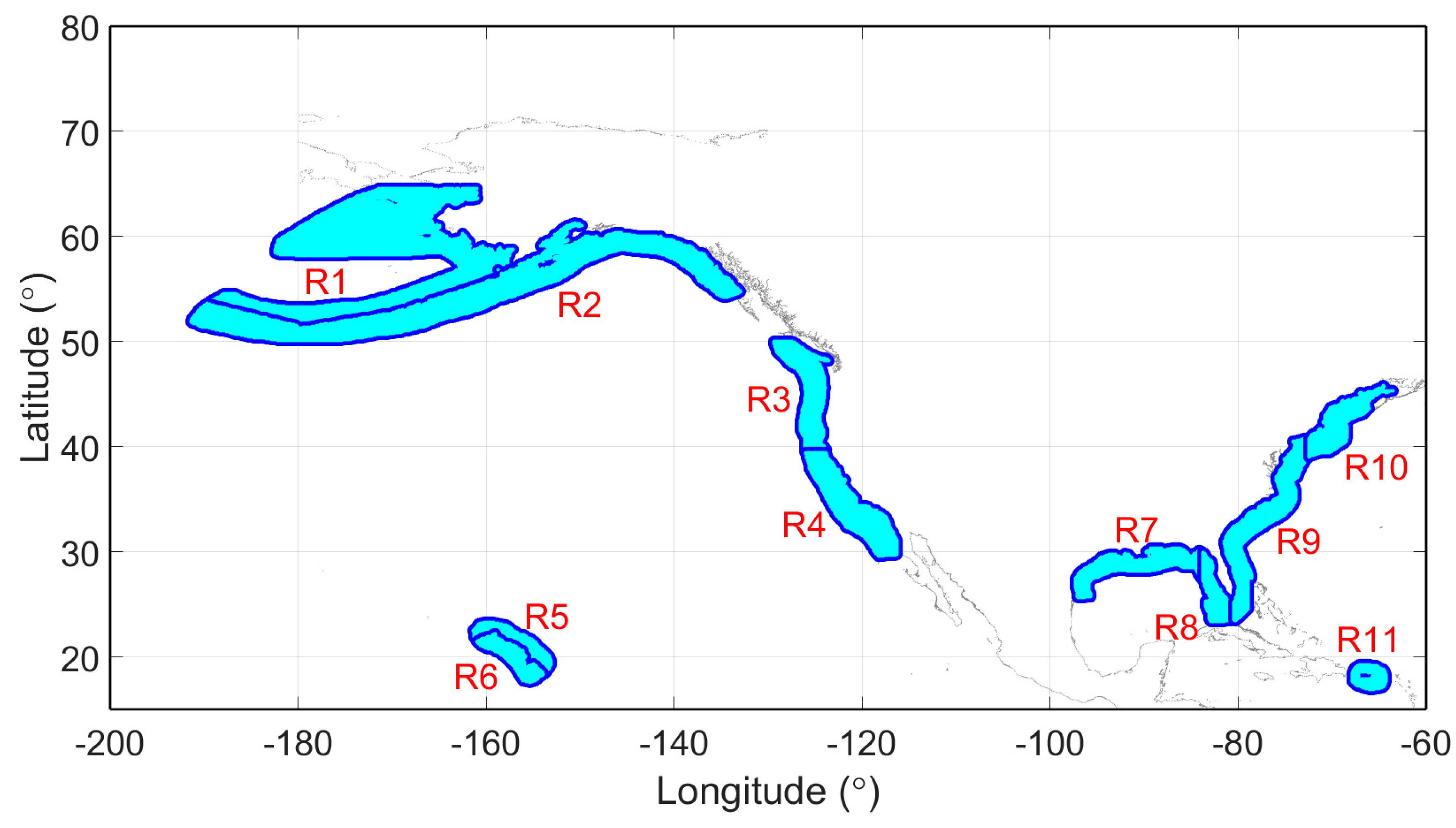
Given the importance of the distribution of the available wave energy, $AAE$, over peak period, direction, and time (season) on the design and operation of WECs, investigations of $AAE$ as a function of these variables are conducted herein to provide additional insights on wave climates and energy resources in US coastal waters. The present study plots and analyzes marginal distributions, conditional resource parameters, and joint distributions to provide regional wave energy resource characterization and assessment for eleven wave climate regions delineated by Ahn et al. [29]. In this delineation (Figure 1), distinct wave climates in Alaska, the West Coast, Hawaii, the Gulf of Mexico, the East Coast, and Puerto Rico were identified based on the orientation of the coastal waters to dominant wind systems and exposure to swell. The marginal distributions for $AAE$ are mapped in terms of peak period bin ($T_b$), direction bin (${\theta }_b$), and month ($M$). The joint distributions for $AAE$ are mapped as a function of two of these three variables and are used to derive the conditional resource parameters characterizing peak period spread, directionality coefficient, and seasonal variability conditional on the variables ($T_b,{\theta }_b,M$). These marginal and joint distributions as well as the conditional resource parameters for each region are presented in Figure 2, Figure 3, Figure 4, Figure 5, Figure 6, Figure 7, Figure 8, Figure 9, Figure 10, Figure 11 and Figure 12.

The parameter $\langle AAE\left(T_b,{\theta }_b,M\right)\rangle$ denotes the spatially averaged regional distribution that is computed by averaging all the 30 year averaged $AAE$ values, $AAE\left(T_b,{\theta }_b,M\right)$, within a given region. The spatially averaged regional joint distribution, as a function of period and direction bins, is then computed by summing across all months, e.g., $\langle AAE\left(T_b,{\theta }_b\right)\rangle ={\displaystyle \sum }_M\langle AAE\left(T_b,{\theta }_b,M\right)\rangle$. This distribution is shown in the upper-left hand corner of Figure 2, Figure 3, Figure 4, Figure 5, Figure 6, Figure 7, Figure 8, Figure 9, Figure 10, Figure 11 and Figure 12. Similarly, the joint distribution for $AAE$ as a function of month and direction (lower-left hand corner) and the joint distribution as a function of month and period (upper-right hand corner) are determined. The three averaged regional marginal distributions, $\langle AAE\left(T_b\right)\rangle$, $\langle AAE\left({\theta }_b\right)\rangle$, and $\langle AAE\left(M\right)\rangle$ are inserted adjacent to the joint distributions in Figure 2, Figure 3, Figure 4, Figure 5, Figure 6, Figure 7, Figure 8, Figure 9, Figure 10, Figure 11 and Figure 12. Note that a grand sum of each marginal or joint distribution is the total averaged $AAE$ within each region.

Results from these joint distributions indicate how much $AAE$ is associated with a given wave system, e.g., $AAE$ for a wave system characterized by a particular peak period and directional range. The marginal distributions are used to identify the dominant $AAE$ period bands contributing the most energy to the total $AAE$, and the joint distribution,$\langle AAE\left(T_b,{\theta }_b\right)\rangle$, is used to identify the dominant wave systems containing the largest $AAE$ portion. To enhance readability of the descriptions, the dominant wave systems containing the local peaks of energy are illustrated by black boxes over three consecutive bins in both peak period and direction within the joint distribution $\langle AAE\left(T_b,{\theta }_b\right)\rangle$. While this approach of averaging the waves over a large regional scale may mix some of the wave systems, it is able to reveal regional trends. In addition, the wave systems contributing large portions of energy within sub-regions are identified using sub-regional $\langle AAE\left(T_b,{\theta }_b\right)\rangle$ and summarized in geographic maps (lower-right hand corner in Figure 2, Figure 3, Figure 4, Figure 5, Figure 6, Figure 7, Figure 8, Figure 9, Figure 10, Figure 11 and Figure 12. Detailed descriptions of Figure 2, Figure 3, Figure 4, Figure 5, Figure 6, Figure 7, Figure 8, Figure 9, Figure 10, Figure 11 and Figure 12 are provided in Figure 2 caption. The joint distributions, $\langle AAE\left(T_b,M\right)\rangle$ and $\langle AAE\left(M,{\theta }_b\right)\rangle$, are used to describe the seasonal variability of the wave systems with the local and global wind climatology characterized using the Scatterometer Climatology of Ocean Winds (SCOW) [44] based on 10 years of QuikSCAT scatterometer data [45].

The resource parameters for each site as functions of the peak period, direction and month, $d_{\alpha }\left(T_b\right)$, $t_s\left(T_b\right)$, ${ϵ}_{AAE}\left({\theta }_b\right)$, $t_s\left({\theta }_b\right)$, $d_{\alpha }\left(M\right)$, and ${ϵ}_{AAE}\left(M\right)$, are calculated at all sites within a region. The averaged regional resource parameters,$\langle d_{\alpha }\left(T_b\right)\rangle$, $\langle t_s\left(T_b\right)\rangle$, $\langle {ϵ}_{AAE}\left({\theta }_b\right)\rangle$, $\langle t_s\left({\theta }_b\right)\rangle$, $\langle d_{\alpha }\left(M\right)\rangle$, and $\langle {ϵ}_{AAE}\left(M\right)\rangle$, are then calculated by averaging the parameters for all sites in a given region and presented with the corresponding marginal distributions in Figure 2, Figure 3, Figure 4, Figure 5, Figure 6, Figure 7, Figure 8, Figure 9, Figure 10, Figure 11 and Figure 12. For example, $\langle d_{\alpha }\left(T_b\right)\rangle$ is the regional averaged directionality coefficients conditional on the peak period, indicating the directional spread of the wave energy for specific peak period bins. The low value for each parameter indicates a narrow peak period spread, broad directional spread, and low seasonal variability. The value of this approach is that examination of the regional wave energy resource characteristics are primarily focused on the dominant energy bands and wave systems for each region, allowing a more precise characterization and assessment compared to one that includes the total resource in all energy bands. For some regions exhibiting large spatial variability in the wave climates, characteristics of sub-regional dominant wave systems are described using the joint distributions rather than using the regional averaged resource parameters as they provide a broad-brush characterization.

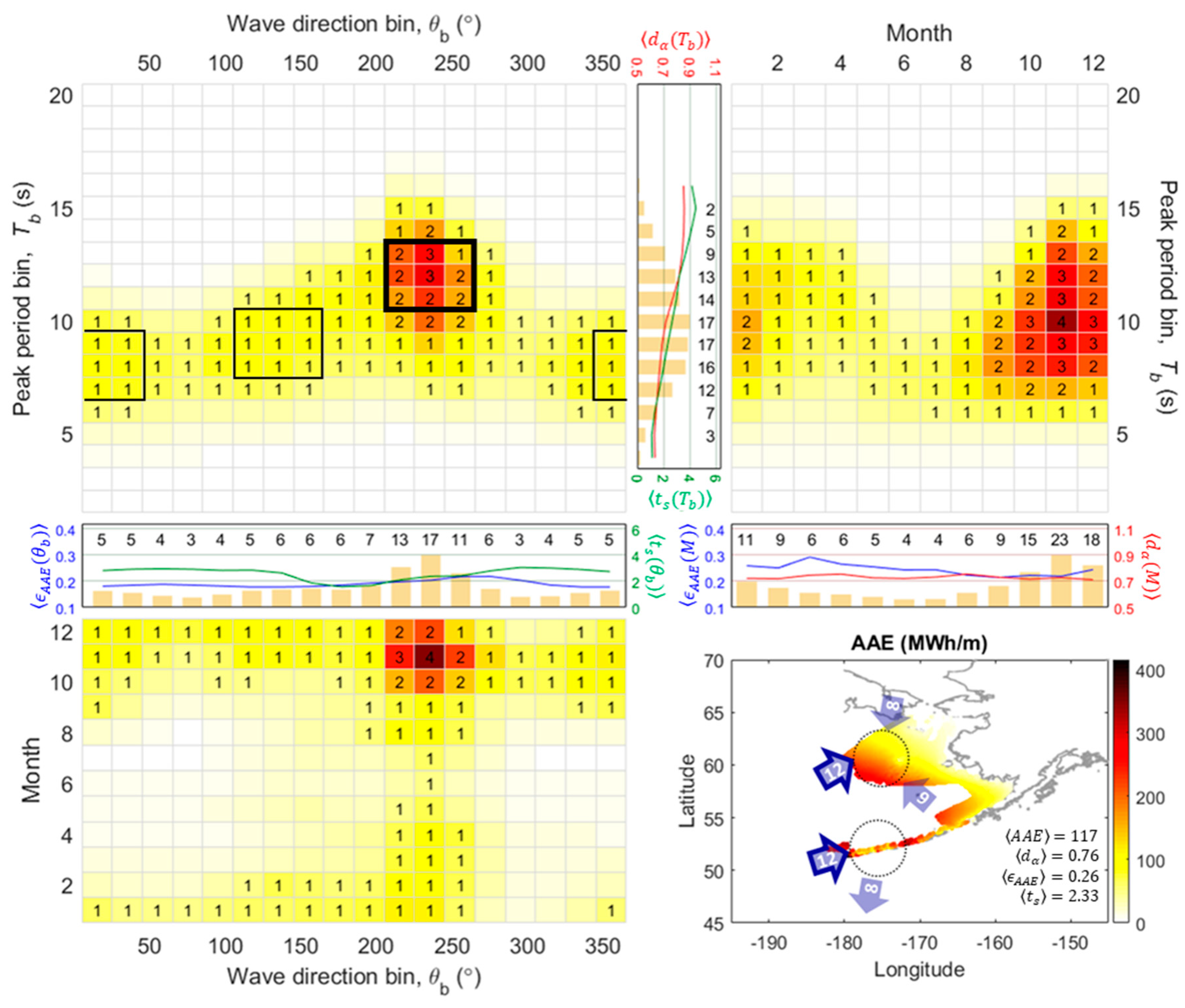
3.1. Region 1: Bering Sea

Wave energy resource attributes of coastal waters in the Bering Sea are illustrated in Figure 2. Spatially averaged values, $\langle AAE\rangle$, $\langle d_{\alpha }\rangle$, $\langle {ϵ}_{AAE}\rangle$, and $\langle t_s\rangle$, which characterize the total wave energy, are shown in Figure 2, lower right-hand corner (117 MWh/m, 0.76, 0.26, 2.33). The wave energy in this region, relative to other US regions, is moderate, exhibiting a moderate peak period spread, a broad directional spread, and a large seasonal variability. This region is further divided into two sub-regions: the west coast of Alaska (latitude > 55) and the Northern side of the Aleutian Islands.

The energy within the marginal distribution for $\langle AAE\left(T_b\right)\rangle$ for the full region is generated from multiple wave systems and is broadly distributed with a sizable amount of energy across periods ranging from wind seas to longer period swells, peaking in the short-period swell band. As seen in the joint distributions marked with the bold box, the dominant wave system present in both sub-regions consists of long-period swells (11–13 s) in late fall (Oct.–Dec.) from SW (200–260°). This wave system is driven by westerlies with prevailing winds, in the marginal sea of the Pacific. The secondary wave systems (thin-line boxes in the joint distribution) consist of short-period swells (7–9 s) from N (340–40°) in late fall (Oct.–Dec.) for both regions and short-period swells (8–10 s) from SE (100–160°) in early winter (Nov.–Jan.) for the west coast of Alaska.

The dominant wave system leads to a larger value for $\langle d_{\alpha }\left(T_b\right)\rangle$ within the swell band, indicating a narrow range of directions with significant energy for both sub-regions. This is compared to the smaller value of $\langle d_{\alpha }\left(T_b\right)\rangle$ within the wind sea and short-period swell bands, indicating a broad range of directions for the secondary wave systems in the west coast of Alaska. The seasonal variation for both sub-regions is characterized by the value of $\langle t_s\left(T_b\right)\rangle$ which is quite large for the dominant and secondary wave systems within the swell periods, but much smaller for the wind seas which are generally present in some form year-round. In the summertime, the wind seas are from SW (200–260°), similar to the dominant wave system. Therefore, the seasonal variability $\langle t_s\left({\theta }_b\right)\rangle$ is small for waves from SW (200–260°) and larger for all other directions. Due to the high energy of the swells in the dominant wave system for both sub-regions, the peak period spread $\langle {ϵ}_{AAE}\left(M\right)\rangle$ for late fall (Oct.–Dec.) is relatively narrow representing a prevailing peak period band during this season. However, because both wind seas and the dominant swells are from SW (200–260°), the peak period spread ${ϵ}_{AAE}\left({\theta }_b\right)$ is relatively broad within this direction band.

The information provided in this analysis further elucidates the wave energy resource attributes that are relevant for WEC design and operation. If a developer targets the dominant wave system in the long-period swell band, this resource has small directional spread but a large seasonal variation. This would permit a simpler and less expensive strategy for design and operation, targeting a narrow peak period band and minimizing the cost of controls to re-tune the WEC, and allowing directionally dependent WECs with less expensive mooring systems [46]. However, the capacity factor would be lower because of the strong seasonal variation. In contrast, a WEC design concept that can operate across a broad band of periods from wind seas to long-period swells using an advanced control system would increase the capacity factor by targeting the dominant wave system as well as the wind sea. Of course, these strategies to increase capacity factor would significantly increase costs, which would have to be weighed against the benefits of increased generation.

3.2. Region 2: Aleutian Trench and Gulf of Alaska

The wave resource characteristics for the Aleutian Trench and the Gulf of Alaska are illustrated in Figure 3. Values for the spatially averaged $\langle AAE\rangle$, $\langle d_{\alpha }\rangle$, $\langle {ϵ}_{AAE}\rangle$, and $\langle t_s\rangle$ which characterize the total wave energy are shown in Figure 3, lower right-hand corner (229 MWh/m, 0.82, 0.22, 1.58). In general, this region has high energy potential with narrow peak period spread, but with broad directional spread, and moderately high seasonal variability. This region is divided into two sub-regions: the southern side of the Aleutian Islands and the Gulf of Alaska. Other than wave directions, the sub-regions exhibit similar wave climates, e.g., peak periods and seasonality.

The majority of the energy in the marginal distribution for $\langle AAE\left(T_b\right)\rangle$ is within the short-period swell band (10–12 s) with much less energy within the wind sea band. The energy distribution for the sub-regions has two swell systems from different directions in winter. The dominant wave system is swell (11–13 s) from S (160–220°) for the southern side of the Aleutian Islands (left circle in map) and SW (200–260°) for the Gulf of Alaska (right circle in map) during winter (Nov.–Jan.). The secondary wave system is shorter-period swells (10–12 s) from SE (100–160°) and S (160–220°) for each sub-region, which are generated by the Aleutian Low-pressure system in winter.

The directionality coefficient $\langle d_{\alpha }\left(T_b\right)\rangle$ is a bit larger for swell periods indicating a narrower distribution of directions for high energy waves, due to the concentration of higher energy within the dominant wave system. The joint distribution for $\langle AAE\left(T_b,M\right)\rangle$ makes it clear that this is particularly true for the swell, but less so for the wind sea peak period band which has more consistent energy throughout the year. This is reflected in a larger $\langle t_s\left(T_b\right)\rangle$ for the swell band than for the wind sea band. The seasonal variability is slightly smaller $\langle t_s\left({\theta }_b\right)\rangle$ for the S (160–220°) because of the presence of wind seas from this direction during summer for both sub-regions. Because the dominant wave system has energy concentrated in the swell band, the peak period spread $\langle {ϵ}_{AAE}\left(M\right)\rangle$ is small during winter (Dec.–Feb.), whereas $\langle {ϵ}_{AAE}\left(M\right)\rangle$ is large during summer (Jun.–Aug.).

As the dominant and secondary wave systems have similar peak periods leading to a narrow peak period spread for these resources, WEC devices can target both systems resonating at similar periods. However, due to the strong seasonal variations of these wave systems, the capacity factor would be low. The capacity factor could be enhanced for both sub-regions by employing omnidirectional WECs or weather-vaning to capture the energy within the short period swell in summer as well. This strategy to increase capacity factor would require a WEC design operating with a broad band of periods from short to long-period swells.

3.3. Region 3: Pacific Northwest Coast

The wave resource characteristics for the Pacific Northwest Coast are illustrated in Figure 4. Values for the spatially averaged $\langle AAE\rangle$, $\langle d_{\alpha }\rangle$, $\langle {ϵ}_{AAE}\rangle$, and $\langle t_s\rangle$ which characterize the total wave energy are shown in Figure 4, lower right-hand corner (340 MWh/m, 0.89, 0.19, 1.67). This region has high energy with narrow directional and peak period spread, but high seasonal variability. The sites in this region have a spatially similar wave energy distribution where coefficients of variation (standard deviation/average) of the resource parameters across the region are fairly low [29].

Looking at the marginal distribution for $\langle AAE\left(T_b\right)\rangle$, the bulk of the energy for this region is contained in the long-period swell band of 12–14 s. The wind sea peak period bands have the least amount of energy. The wave energy within this region generally comes from three wave systems: the dominant wave system (13–15 s) from W (240–300°) during winter (Dec.–Feb.) and the secondary wave systems (9–11 s) from SSW (180–240°) during winter (Dec.–Feb.) and WNW (260–320°) during summer (Jun.–Aug.). The dominant wave system is generated by the westerlies. The directions of the local wind driving the secondary wave systems have a strong seasonality; the local winds blow from NNW during summer (Pacific High) and from SSW during winter (Aleutian Low).

The dominant wave system is largest during early winter (Nov.–Jan.) leading to a large value of $\langle t_s\left(T_b\right)\rangle$ for the swell range. In contrast, the energy in the two secondary wave systems are present year-round, leading to a small value of $\langle t_s\left(T_b\right)\rangle$ for the short-period swell range. Because such a large portion of the swell energy is coming from a narrow range of directions, the directionality coefficient, $\langle d_{\alpha }\left(T_b\right)\rangle$, is quite large for the swell period band. Although the shorter period swell band (9–11 s) has a small value of $\langle d_{\alpha }\left(T_b\right)\rangle$, because the two secondary wave systems in this band completely split into different seasons, this resource exhibits a narrow directional spread. The range of periods containing energy seems to be broader during winter (Dec.–Feb.) than summer (Jun.–Aug.) with the long-period and short-period swells both present; however, because the energy in winter is mostly from the dominant wave system, the peak period spread $\langle {ϵ}_{AAE}\left(M\right)\rangle$ is quite low, whereas in summer, the energy is evenly distributed among all the periods containing energy, leading to a larger $\langle {ϵ}_{AAE}\left(M\right)\rangle$.

The remarkably narrow directional and peak period spread of the dominant wave system allows for a simplification of the device design for fewer frequencies/directions, potentially leading to a decrease in the cost of energy. However, this wave system has significant seasonal variability, WEC technologies targeting the dominant wave system may have low capacity factors in summer, potentially leading to an increase in the cost of energy. Because the long-period swells contain the most energy, WEC technology in this region will need to be relatively large to achieve natural resonance for optimal energy generation [47]. On the other hand, WEC technologies targeting the secondary wave systems in the short-period swell band (9–11 s) would experience a high capacity factor and fewer constraints in the directionality due to the distinct seasonality of these wave systems.

3.4. Region 4: California Coast

The wave resource characteristics for the California coast are illustrated in Figure 5. Values for the spatially averaged $\langle AAE\rangle$, $\langle d_{\alpha }\rangle$, $\langle {ϵ}_{AAE}\rangle$, and $\langle t_s\rangle$ which characterize the total wave energy are shown in Figure 5, lower right-hand corner (190 MWh/m, 0.89, 0.24, 1.17). Overall, this region has a good level of energy, narrow peak period and directional spread, and moderate seasonal variation. Like R3, the sites in this region have a spatially similar wave energy distribution.

The marginal distribution for $\langle AAE\left(T_b\right)\rangle$ has the largest amount of energy in the swell period band (13–15 s), with moderate energy retained in the short-period swell band (9–11 s). The long-period swells contain two very different wave systems. The dominant system with the most energy is the North Pacific swells (13–15 s) from W (240–300°) in winter (Dec.–Feb.), whereas the secondary wave system is Southern Hemisphere swells (14–16 s) from S (160–220°) during the non-winter months. The short-period swell band contains another secondary wave system, 9–11 s from WNW (260–320°) during early summer (May–Jul.). The local wind in this region blows from the northwest (Pacific High) throughout the year in contrast to the local wind direction in Pacific Northwest Coast which has strong seasonality. This climatological discontinuity is located at the boundary between the two regions as well as the boundary between the Cascadia Subduction Zone and the San Andreas Fault. Notably, the local wind speed in this region is larger during summer than winter [45].

The seasonal variation of the long-period swell, containing the dominant wave system, is a little larger than the seasonality of the short-period swells, containing the secondary wave system, as reflected by a slightly larger $\langle t_s\left(T_b\right)\rangle$ for the long-period swell band. The swells from the Southern Hemisphere have a much smaller $\langle t_s\left({\theta }_b\right)\rangle$, because most months have very similar magnitudes of energy for those swells. Because the wave systems are distributed within the narrow directional band (240–320°), the directionality coefficient $\langle d_{\alpha }\left(T_b\right)\rangle$ in both short and long-period swell bands is fairly large. The wave systems show large seasonality in both peak period spread and directional spread. In winter, the energy is mainly from the dominant wave system, leading to a narrow peak period $\langle {ϵ}_{AAE}\left(M\right)\rangle$ and directional spread $\langle d_{\alpha }\left(M\right)\rangle$. In summer, the two secondary wave systems exhibiting different period and direction bands lead to a broad peak period spread $\langle {ϵ}_{AAE}\left(M\right)\rangle$ and directional spread $\langle d_{\alpha }\left(M\right)\rangle$ during those months.

The wave systems are generated from similar directions, and exhibit the least directional spread among the US wave climates, enabling a simpler device design that can operate in a narrow band of directions, potentially leading to a decrease in the cost of energy in this region. Because the energy for the dominant wave system does vary seasonally, the capacity factors would be less than ideal for devices only targeting those periods. However, the capacity factor could be improved by utilizing WECs that are able to respond to a broader range of peak periods to maximize the energy conversion due to the shift in dominant peak periods from the long-period swells (13–15 s) in winter to the short-period swells (9–11 s) in summer.

3.5. Region 5: Hawaiian—Northern Coast

The wave resource characterizations for the northern Hawaiian coast are shown in Figure 6. Values for the spatially averaged $\langle AAE\rangle$, $\langle d_{\alpha }\rangle$, $\langle {ϵ}_{AAE}\rangle$, and $\langle t_s\rangle$ which characterize the total wave energy are shown in Figure 6, lower right-hand corner (143 MWh/m, 0.79, 0.25, 1.41). This region has a moderate level of energy and narrow peak period spread, but moderate directional spread and seasonality. This region is further divided into three sub-regions: west (Kauai and Niihau), center (Oahu and Maui), and east (Hawaii).

As seen in the joint distributions marked with the bold box, the dominant wave system for these sub-regions consists of long-period swells (13–15 s) from NNW (300–260°) in winter (Dec.–Feb.) and short-period swells (8–10 s) from ENE (40–100°) nearly year-round. The relative importance of the two wave systems is different for each of these sub-regions. For the western sub-region (left circle in map), the long-period swells (13–15 s) from NNW (300–360°) are the dominant contributor to the overall energy, whereas for the eastern sub-region (right circle in map) the short-period swells (8–10 s) from ENE (40–100°) dominate. In the central sub-region (middle circle in map), both wave systems have significant contributions to the overall wave energy. The year-round short-period swells are generated by the NE trade winds and are a mix of wind seas and short-period swells, whereas the long-period swells are generated by the westerlies arriving from a long distance across the North Pacific Ocean in winter.

Because the short-period swells occur year-round, the seasonal variability, $\langle t_s\left(T_b\right)\rangle$ and $\langle t_s\left({\theta }_b\right)\rangle ,$ is quite low for 8–10 s and ENE band. In contrast, the long-period swells have high seasonal variability. The energy for both wave systems is contained in a fairly modest range of peak periods, with slightly more spread for the short-period swells as indicated by values of $\langle {ϵ}_{AAE}\left({\theta }_b\right)\rangle$ on the order of 0.2 compared to $\langle {ϵ}_{AAE}\left({\theta }_b\right)\rangle$ around 0.15 for the long-period swells. In addition, during summer, the energy from the short-period swells shift to a shorter period as the waves are comprised of more wind seas rather than swells. The range of directions for the short-period swells is quite broad, reminiscent of wind seas, compared to the long-period swell where the short-period swells have small $\langle d_{\alpha }\left(T_b\right)\rangle$ compared to the long-period swells. This leads to a strong seasonal variability in the directional spread where $\langle d_{\alpha }\left(M\right)\rangle$ is relatively large during winter (Dec.–Feb.), whereas $\langle d_{\alpha }\left(M\right)\rangle$ is small during summer (Jun.–Aug.).

WEC devices targeting the short-period swells driven by the trade winds would need to be able to respond to a broader range of peak periods and would face more constraints based on a broad range of directions, whereas devices targeting the long-period swells driven by westerlies have fewer constraints on both the period and directions. However, due to the strong seasonality of the long-period swells, WEC devices targeting them would experience higher seasonal variability (lower capacity factor), potentially leading to an increase in the cost of energy. The particular choice of WEC technology varies for different sub-regions.

3.6. Region 6: Hawaiian—Southern Coast

The wave resource characteristics for the southern Hawaiian coast are illustrated in Figure 7. Values for the spatially averaged $\langle AAE\rangle$, $\langle d_{\alpha }\rangle$, $\langle {ϵ}_{AAE}\rangle$, and $\langle t_s\rangle$ which characterize the total wave energy are shown in Figure 7, lower right-hand corner (43 MWh/m, 0.81, 0.33, 0.82). This region has a lower level of energy, broad peak period spread, moderate directional spread, and low seasonal variability. Notably, sub-regions of this region, defined in the R5 (northern Hawaiian coast), have a spatially similar wave energy distribution, like occurs in R3 (Pacific Northwest Coast) and R4 (California coast).

Like R5, the marginal distribution $\langle AAE\left(T_b\right)$ has two peaks with similar contributions to total $\langle AAE\rangle$ for the full region: 7–10 s waves and 13–15 s waves. The energy distribution in this region has three separate wave systems that equally contribute to $\langle AAE\rangle$; the short-period swells (7–9 s) driven by trade winds from ENE (40–100°) almost year-round, the Southern Hemisphere generated long-period swells (14–16 s) from S (160–220°) during non-winter months (Apr.–Oct.), and the North Pacific swells (13–15 s) from NW (280–340°) during winter (Dec.–Feb.). The swells from S (160–220°) are generated by the South Pacific winter storms from Australia and New Zealand [48]. The trade winds swell and North Pacific swell systems have a broader peak period spread and high seasonal variability compared to the same wave systems in R5.

These wave systems show distinct characteristics as seen in $\langle {ϵ}_{AAE}\left({\theta }_b\right)\rangle$ and $\langle t_s\left({\theta }_b\right)\rangle$: the ENE (40–100°) short-period swells exhibit a relatively broad peak period spread $\langle {ϵ}_{AAE}\left({\theta }_b\right)\rangle$ and low seasonal variability $\langle t_s\left({\theta }_b\right)\rangle$, the S (160–220°) long-period swells exhibit relatively narrow peak period spread and low seasonal variability, the NW (280–340°) long-period swells exhibit relatively broad peak period spread and large seasonal variability. As seen in the joint distribution for $\langle AAE\left(T_b,M\right)\rangle$, the energy in the long-period band (13–15 s) is only slightly larger in winter (Dec.–Feb.) and the energy in the lower period band is fairly consistent year-round. Due to the absence of the NW (280–340°) swells during summer, the directionality coefficient, $\langle d_{\alpha }\left(M\right)\rangle$, is slightly increased due to the waves coming from a relatively narrower range of directions for this season. In contrast, because there is energy within both swell and wind sea periods throughout the year, the peak period spread $\langle {ϵ}_{AAE}\left(M\right)\rangle$ is fairly constant.

Like R5, wave energy projects in R6 would select suitable WEC technologies with natural resonance properties that are designed for power absorption of the dominant wave energy systems within distinct period and directional bands, which are occurring in different seasons. This is challenging in regions like Hawaii where there are multiple dominant wave systems. Omnidirectional or weather-vaning WECs targeting the long period swells would experience a higher capacity factor. For directionally dependent WEC technologies, targeting the South Pacific swells would have the most narrow peak period and directional spread and low seasonal variability among the three-wave systems. The short-period swells driven by trade winds may still be viable for projects that require relatively small-scale WEC devices with a steady supply.

3.7. Region 7: Gulf of Mexico—Western and Central Coast

The wave resource characteristics for the Gulf of Mexico (western and central coast) are illustrated in Figure 8. Values for the spatially averaged $\langle AAE\rangle$, $\langle d_{\alpha }\rangle$, $\langle {ϵ}_{AAE}\rangle$, and $\langle t_s\rangle$ which characterize the total wave energy are shown in Figure 8, lower right-hand corner (32 MWh/m, 0.77, 0.28, 1.09). This region has low energy with a broad period and directional spread, but moderately low seasonal variations. This region is divided into two areas: the western and central coasts in the Gulf of Mexico.

Based on the marginal distribution for $\langle AAE\left(T_b\right)\rangle$, the energy for this region is concentrated within the wind sea band (6–8 s). The waves are from a broad range of directions, with the highest concentration of energy being from SE (100–160°). The dominant wave system is generated from SE (100–160°) for the western coast (left circle in map) and SSE (120–180°) for the central coast (right circle in map) during non-summer months (Oct.–May). There is a low level of energy in the swell band (12–14 s) for SE (100–160°) during the late summer (Aug.–Sep.) along the central coast, which is generated by tropical cyclones from the Atlantic basin.

In the central coast, these wave systems lead to a small value for $\langle t_s\left({\theta }_b\right)\rangle$ within the SE (100–160°) band and the waves from the other directions have stronger seasonal dependence, and hence larger variabilities. The peak period spread is the largest during late summer (Jul.–Sep.), $\langle {ϵ}_{AAE}\left(M\right)\rangle$, and for waves from SE (100–160°), $\langle {ϵ}_{AAE}\left({\theta }_b\right)\rangle$ for this sub-region, because of the presence of swells. As the dominant wave system is slightly larger in spring (Mar.–May), the directionality coefficient, $\langle d_{\alpha }\left(M\right)\rangle$, is large in this season for both sub-regions when the winds tend to be more persistent.

The sites located on the western coast would only be considered for small-scale applications due to the overall small potential. For this region, WEC technologies operating within the wind sea band would have the largest capacity factor due to the relatively weak seasonal variation. Therefore, the WEC technologies designed for this region would be relatively small to achieve natural resonance for optimal energy capture.

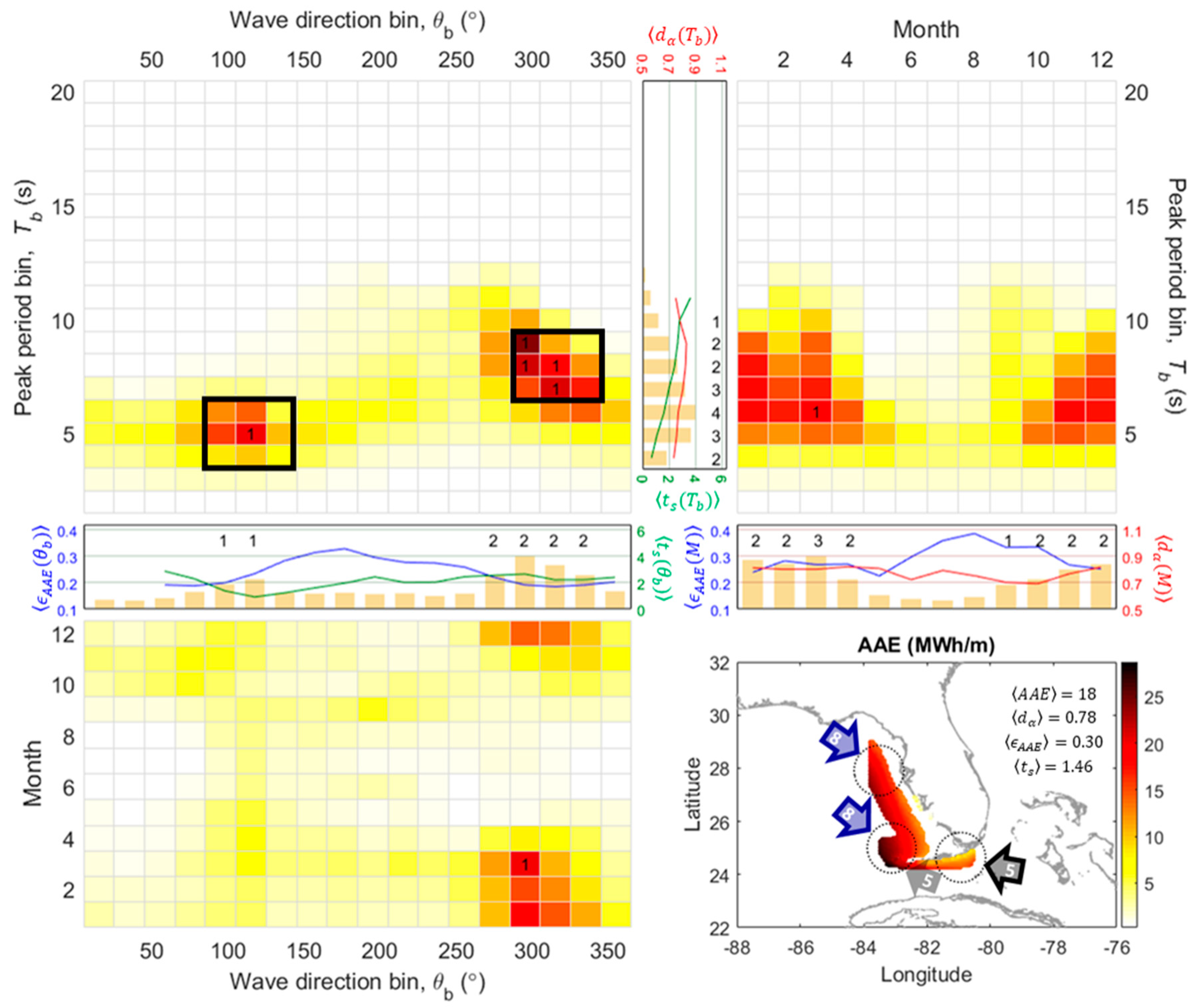
3.8. Region 8: Gulf of Mexico—Eastern Coast

The wave resource characteristics for the Gulf of Mexico (eastern coast) are illustrated in Figure 9. Values for the spatially averaged $\langle AAE\rangle$, $\langle d_{\alpha }\rangle$, $\langle {ϵ}_{AAE}\rangle$, and $\langle t_s\rangle$ which characterize the total wave energy are shown in Figure 9, lower right-hand corner (18 MWh/m, 0.78, 0.3, 1.46). This region has the lowest total wave energy with a broad peak period spread along with moderate directional spread and seasonal variability. This region is divided into three sub-regions: the Florida Shelf, the Florida Keys, and the corner transition between the two sub-regions.

As seen in the marginal distribution for $\langle AAE\left(T_b\right)\rangle$, the energy for this region is concentrated in the wind sea and short-period swell regime (4–9 s). The waves are from the full range of directions as seen in the distribution for $\langle AAE\left({\theta }_b\right)\rangle$, with peaks of concentrated energy from ESE (80–140°) and WNW (260–340°). The two dominant wave systems contribute to $\langle AAE\rangle$ within different sub-regions: the dominant wave system in the Florida Shelf (upper circle in map) is the short-period swell (7–9 s) from NW (280–340°) in late winter (Jan.–Mar.), whereas the local wind seas (4–6 s) from ESE (80–140°) nearly year-round is the dominant wave system for the Florida Keys (lower circle in map). The corner area (middle circle in map) has both wave systems, but the longer period waves from NW (280–340°) in late winter dominate.

The wind seas from ESE (80–140°) occur nearly year-round with a constant level of energy. Hence, the seasonal variability, $\langle t_s\left({\theta }_b\right)\rangle$ and $\langle t_s\left(T_b\right)\rangle$, is small for this range of periods and directions. In contrast, the short-period swells from NW (280–340°) are largest in late winter (Jan.–Mar.) and smallest in early summer (May–Jul.) resulting in a much larger $\langle t_s\left({\theta }_b\right)\rangle$ and $\langle t_s\left(T_b\right)\rangle$ from this period and direction band. The peak period spread, $\langle {ϵ}_{AAE}\left({\theta }_b\right)\rangle$, is lower for the directions of the dominant wave systems because the energy is concentrated within a small range of periods. As the short-period swell band is mainly contributed by the NW (280–340°) waves, this resource band exhibits a relatively large directionality coefficient, $\langle d_a\left(T_b\right)\rangle$, compared to those for the wind sea period band.

Because of the low energy, this region can only be considered for small-scale projects. Obviously, WECs would need to target the wind sea period band. In the Florida Shelf sub-region, projects would experience fewer constraints on directionality but larger constraints on the seasonality. Down in the Florida Keys, projects would have low total energy but with a high capacity factor. This compact and high-efficiency project can be merged with the other renewable energy resource projects, e.g., wind energy and ocean current energy.

3.9. Region 9: Atlantic—South and Mid-Coast

The wave resource characteristics for the south and mid-Atlantic coast are illustrated in Figure 10. Values for the spatially averaged $\langle AAE\rangle$, $\langle d_{\alpha }\rangle$, $\langle {ϵ}_{AAE}\rangle$, and $\langle t_s\rangle$ which characterize the total wave energy are shown in Figure 10, lower right-hand corner (65 MWh/m, 0.77, 0.27, 0.88). This region generally has a moderate level of energy and peak period spread with the broad directional spread but low seasonal variability. This region is divided into two sub-regions: the south and mid-Atlantic and the Florida Channel between Florida and the Bahamas.

The marginal distribution for $\langle AAE\left(T_b\right)\rangle$ indicates that the energy for this region is distributed between wind seas and short-period swells. Based on the distribution for $\langle AAE\left({\theta }_b\right)\rangle$, the waves are arriving from a range of directions with peaks from NE and SE (40–140°). In the Florida Channel (lower circle in map), the most dominant wave system is the wind seas (6–8 s) from NE (20–80°) in winter (Dec.–Feb.). The south and mid-Atlantic coast (upper circle in map) have three wave systems: the two dominant wave systems, the short-period swells (9–11 s) from ENE (40–100°) driven by nor’easters in non-summer months (Sep.–May) and the year-round short-period swells (8–10 s) from ESE (80–140°) driven by trade winds (or Bermuda High-pressure system), and a secondary wave system (6–8 s) from S (140–200°) in late winter (Jan.–Mar.).

As the trade winds (or Bermuda High-pressure system) swells are generated nearly year-round, the seasonal variability, $\langle t_s\left({\theta }_b\right)\rangle$, is smaller for ESE (80–140°) band than for ENE (40–100°) band for south- and mid-Atlantic coast. This wave system contributes to the energy for the short-period swell band in summer, leading to small seasonal variability, $\langle t_s\left(T_b\right)\rangle$, within this period band. Because the two short-period swell systems are roughly generated from a similar direction, the directionality coefficient, $\langle d_{\alpha }\left(T_b\right)\rangle$, for their period band is fairly large.

Although the total wave energy for this region exhibits relatively broad directional spread, the energy within the dominant wave systems is distributed in the narrow directional band, 40–140° for south and mid-Atlantic coast and 20–80° for the Florida Channel, reducing the importance of the wave directionality. In the south and mid-Atlantic coast, WEC devices targeting the swells driven by both trade winds (or Bermuda High-pressure system) and nor’easters, would experience fewer constraints on both seasonality and directionality. High capacity factors may be expected due to remarkably small seasonal variability. Like R8, the energy projects in the Florida Channel can also be merged with other ocean renewable resources due to the presence of local winds and persistent ocean currents.

3.10. Region 10: Atlantic—North Coast

The wave resource characteristics for the Atlantic (north coast) are illustrated in Figure 11. Values for the spatially averaged $\langle AAE\rangle$, $\langle d_{\alpha }\rangle$, $\langle {ϵ}_{AAE}\rangle$, and $\langle t_s\rangle$ which characterize the total wave energy are shown in Figure 11, lower right-hand corner (83 MWh/m, 0.74, 0.26, 1.05). This region has a moderate level of wave energy and peak period spread with broad directional spread and low seasonal variability. Like R3 (Pacific Northwest Coast), R4 (California coast), and R6 (southern Hawaiian coast), the sites in this region have spatially similar wave energy distributions.

Like the southern part of the East Coast, the marginal distribution for $\langle AAE\left(T_b\right)\rangle$ shows that there is significant energy in both the wind sea and short-period swell ranges. The distribution for $\langle AAE\left({\theta }_b\right)\rangle$ indicates energy in a broad range of directions with multiple peaks in 80–220° directions along with a little peak from W (240–300°). Most sites have two dominant wave systems with similar contributions to total $\langle AAE\rangle$: the short-period swells (8–10 s) from S (160–220°) in winter to spring (Nov.–Apr.) driven by the Burmuda high-pressure system and the short-period swells (9–11 s) from ESE (80–140°) in non-summer months (Sep.–May) driven by nor’easters. A secondary wave system, wind seas (6–8 s) from W (240–300°) during winter (Dec.–Feb.) generated by westerlies, also contributes to the wave energy for this region.

Although these wave systems are dominant in winter, short-period local wind sea contains considerable energy in the summer, which decreases the seasonal variability for this region. As these summer wind seas are mainly coming from the south, the seasonal variability $\langle t_s\left({\theta }_b\right)\rangle$ is small and the peak period spread $\langle {ϵ}_{AAE}\left({\theta }_b\right)\rangle$ is large for the 140–220° band containing the Burmuda high-pressure swell system. The W (240–300°) westerlies wind seas are only present during winter within a narrow peak period range, giving a larger $\langle t_s\left({\theta }_b\right)\rangle$ and smaller $\langle {ϵ}_{AAE}\left({\theta }_b\right)\rangle$ within this directional band. The wave directions of the two dominant wave systems are roughly perpendicular to each other, leading to the broad directional spread of the total wave energy for this region.

Directionally dependent WEC technologies would need advanced controls for this region because of the relatively broad directional spread derived from the two dominant wave systems. WEC devices targeting the swells from ESE (80–140°) driven by nor’easters would have high seasonal variability (low capacity factor). WEC devices targeting the swells from S (160–220°) driven by the Burmuda high-pressure system would need to be able to respond to the wind seas to increase capacity factor. To improve the capacity factor, omnidirectional WEC devices targeting both wave systems in 8–11 s period could be utilized.

3.11. Region 11: Puerto Rico

The wave resource characteristics for the Puerto Rico coast are illustrated in Figure 12. Values for the spatially averaged $\langle AAE\rangle$, $\langle d_{\alpha }\rangle$, $\langle {ϵ}_{AAE}\rangle$, and $\langle t_s\rangle$ which characterize the total wave energy are shown in Figure 12, lower right-hand corner (39 MWh/m, 0.89, 0.27, 1.10). This final region has low energy, but moderate peak period spread and seasonal variability, and low directional spread. Like the Hawaiian regions, this region is roughly divided into the northern and southern coast: the Atlantic Ocean side and the Caribbean Sea side.

The marginal distribution for $\langle AAE\left(T_b\right)\rangle$ clearly shows that the energy for this region spans the full range of wind sea and swell periods. There are peaks in this distribution within the wind sea range and the short-period swell range. The Atlantic Ocean side (upper circle in map) has two dominant wave systems with similar contributions to the total $\langle AAE\rangle$: nor’easter swells (10–12 s) from N (340–40°) in early winter to late winter (Nov.–Mar.) and the trade wind swells (7–9 s) from NE (20–80°) throughout the year. On the other hand, the Caribbean Sea side (lower circle in map) is mainly dominated by local wind seas (5–7 s) from ESE (80–140°) throughout the year.

The wind seas (5–8 s) in both NE (20–80°) and ESE (80–140°) systems are present throughout the year as reflected in the small value for the seasonal variability within this period range $\langle t_s\left(T_b\right)\rangle$. This is contrasted with the nor’easter swells from N (340–40°) which have more energy in winter, giving a larger $\langle t_s\left(T_b\right)\rangle$. Each wave system has narrow directional spread as seen in $\langle d_{\alpha }\left(T_b\right)\rangle$ and is distributed in a similar directional band, leading to a large directionality coefficient of the total wave energy for this region. The directional spread tends to be broader (smaller $\langle d_{\alpha }\left(M\right)\rangle$) during summer (Jun.–Aug.) when there is little swell and the energy is primarily contained in the wind seas. Because the nor’easter swells contain little energy in the wind sea bands, the peak period spread is narrow, giving a low value for $\langle {ϵ}_{AAE}\left({\theta }_b\right)\rangle$ in the N (340–40°) direction. On the other hand, the other wave systems have a much broader peak period spread due to the mix of wind seas and swells.

Different wave energy planning and WEC designs may be required for the Atlantic Ocean side coast and the Caribbean Sea side. On the Atlantic Ocean side, if an energy project emphasizes a constant energy generation (high capacity factor), targeting WEC technologies with an idealized operating period of 7–9 s would maximize the capacity factor. However, if an energy project targets the nor’easter swells (10–12 s) to extract from the higher energy waves, the capacity factor of the project would be decreased. On the other hand, on the Caribbean Sea side, the WEC should operate at the wind sea period. Although the energy potential is relatively low in this sub-region, the year-round wave system is distributed within a narrow direction/period, allowing for a simplification of the device design, and potentially leading to a higher capacity factor in this region.

4. Summary

The joint distributions of $\langle AAE\rangle$ shown in Section 3 reveal dominant wave systems within each of the eleven wave climate regions as summarized in

Table 1. Summary of the characteristics of the dominant wave systems (marked with the black bold box in Figure 2, Figure 3, Figure 4, Figure 5, Figure 6, Figure 7, Figure 8, Figure 9, Figure 10, Figure 11 and Figure 12) in US wave energy regions. Three columns delineate the wave systems based on the peak period, with wave direction, and month in parentheses.

Regions		Wind Sea ${\mathit{T}}_{\mathit{p}}\le 7\mathit{s}$	Short Swell $7\mathbf{s}<{\mathit{T}}_{\mathit{p}}\le 12\mathit{s}$	Long Swell $12\mathbf{s}<{\mathit{T}}_{\mathit{p}}$
R1:	Bering Sea	-	-	SW (10–12)
R2:	Aleutian Trench and Gulf of Alaska	-	-	SSW (11–1)
R3:	Pacific Northwest Coast	-	-	W (12–2)
R4:	California Coast	-	-	W (12–2)
R5:	Hawaiian—Northern Coast	-	ENE (All)	NNW (12–2)
R6:	Hawaiian—Southern Coast	-	ENE (All)	NW (12-2), S (4–10)
R7:	Gulf of Mexico—Western and Central	SSE (10–5)	-	-
R8:	Gulf of Mexico—Eastern	ESE (All)	NW (1–3)	-
R9:	Atlantic—South and Mid-Coast	-	ENE (9–5), ESE (All)	-
R10:	Atlantic—North Coast	-	ESE (9–5), S (11–4)	-
R11:	Puerto Rico	-	NE (All), N (11–3)	-

. For coastal waters in the Bering Sea and the Pacific Ocean (R1–R4), long-period swell systems with a peak period exceeding 12 s in winter contribute most to the total energy, but over a range of wave directions: emanating from the SW direction for the Bering Sea (R1), from the SSW direction for the Aleutian Trench and Gulf of Alaska (R2), and from the W direction for the Pacific Northwest (R3) and California (R4). Coastal waters in Hawaii (R5 and R6) have bi-modal and tri-modal distributions with three major wave systems. The northern coastal Hawaiian waters (R5) have winter season long-period swells originating from NNW and year-round short-period swells originating from ENE. The southern coastal waters (R6) have an additional wave system during non-winter months, consisting of long-period swells originating from S. In the Gulf of Mexico, non-summer wind seas from SSE for the western and central region (R7) and late winter short-period swells from NW for the eastern region (R8) contain the most energy. Like coastal waters around Hawaii, the Atlantic Ocean regions (R9–R11) have multiple wave systems. Those in the south and mid-Atlantic (R9) have two dominant wave systems consisting of short-period swells originating from ENE in non-summer months and ESE year-round. Coastal waters in the North Atlantic (R10) have two dominant short-period swells originating from S in winter to spring and ESE in non-summer months. Coastal waters in Puerto Rico (R11) have two separate dominant wave systems: winter season short-period swells originating from N and year-round short-period swells originating from NE.

5. Conclusions

The annual available energy ($AAE$) partitioned by the peak period, direction, and month is computed using spectral partitioned bulk wave data obtained from a 30 year WaveWatch III (Phase II, ver. 5.08) hindcast. Joint distributions of $AAE$ reveal dominant wave systems within each of the eleven wave climate regions. Marginal distributions and conditional resource parameters show dominant resource bands and how important wave resource characteristics can vary with direction, frequency, and seasonal, e.g., how directional spreading varies seasonally, or how frequency spreading varies over the wave direction. These parameters enable delineation of individual wave systems, and, therebye, a high-fidelity characterization of the resource and a more lucid assessment of the opportunities and constraints for wave energy project development.

The resource characterization and assessment conducted in the present study provide important information for WEC technology developers on the dominant conditions within each of the regions such that they can develop WEC concept designs and strategies that are most effective for a given region. This is a significant benefit, allowing developers to target the most common range of conditions present for US coastal waters. In addition, another key contribution of this study is that it suggests a new methodology for identifying and characterizing the dominant wave systems. However, risks to installation, operation and maintenance (IO&M), and survival should be investigated and characterized based on extreme wave conditions. The regional analysis presented herein sometimes blends conditions over spatially heterogeneous domains. Therefore, the $AAE$ distributions presented herein are not fully representative of specific conditions at individual locations, but, rather, represent the full range of conditions within the individual regions. Creating distributions and performing analyses representative of conditions at specific locations would require the delineation of more sub-regions, perhaps hundreds, for the US, which is beyond the scope of this study. However, similar resource characterizations and assessments using these techniques can be conducted within smaller sub-regions or at a project site. Further, these same analyses can be conducted with higher-resolution model hindcasts for feasibility and design-level resource assessments.