Bi-level Capacity Planning of Wind-PV-Battery Hybrid Generation System Considering Return on Investment

Abstract

Reasonable configuration of equipment capacity can effectively improve the economics of wind-photovoltaic-battery hybrid generation system (WPB-HGS). Based on the current needs of investors to pay more attention to the economic benefits of WPB-HGS, this paper proposes a capacity configuration method for WPB-HGS considering return on investment (ROI). A bi-level planning model for integrated planning and operation of WPB-HGS was established. The lower-level model optimizes the system’s operating status with the goal of maximizing the daily power sales of the system. The upper-level model plans the equipment capacity of the WPB-HGS with the goal of maximizing the annual net income and return on investment. The model is solved using adaptive weighted particle swarm optimization. According to actual engineering examples, the specific equipment capacity is configured, and the configuration results are analyzed to verify the effectiveness of the method.

1. Introduction

With the overexploitation of fossil energy such as oil and coal, the problem of energy exhaustion is becoming more and more serious [1]. Moreover, the economy is developing rapidly all over the world, and the population is growing too fast, resulting in an increasing demand for resources. Therefore, traditional fossil energy has been difficult to meet the needs of economic development. Due to the excessive use of fossil energy, the global ecological environment has been greatly damaged [2]. In order to deal with the problem of energy depletion, all countries in the world have made great efforts to develop environmentally friendly renewable energy (RE) to replace traditional fossil energy [3]. Therefore, photovoltaic (PV), wind energy, tidal energy, and other renewable energy appear in people’s vision. Renewable energy exists in nature, which is inexhaustible and widely distributed, and its impact and damage on the environment can be almost ignored. Because of the above advantages, renewable energy has been widely used. Vigorously developing renewable energy is a key step to alleviate the current shortage of fossil resources such as coal, reduce environmental degradation, and reform of energy structure.

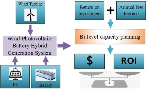
Wind generation and photovoltaic generation are two kinds of renewable energy power generation technologies with the best development prospect and the most extensive application in recent years, which have been highly concerned by all countries in the world [4,5]. The wind-PV hybrid generation system (WP-HGS), which is a combination of wind and photovoltaic generation technology, can combine the complementarity of wind energy and solar energy in time and space, making full use of the natural advantages of both. There is a good complementarity between the two kinds of energy in time and season. So, compared with the wind or photovoltaic generation alone, the WP-HGS has a better stability. At the same time, wind and PV can also have good complementarity in space, which can effectively save the floor space of the system. Compared with the single PV or wind generation system, the WP-HGS can make up for the shortcomings of continuity and discontinuity in the single energy system [6].

With the continuous improvement of the installed capacity of WP-HGS, more and more problems are exposed. First of all, wind and PV generation are intermittent and random with the change of wind and solar [7,8]. The output power is not easy to control, which has a great impact on the power grid and is not conducive to the stability of the power system. Secondly, the growth rate and installed capacity of wind and photovoltaic generation grow too fast, while the grid connected capacity is limited, resulting in a large number of wind and solar abandonment phenomena, which will also lead to the increase of generation cost. At present, in order to solve the above problems, large-scale energy storage devices are usually used in combination with WP-HGS [9]. At present, common energy storage methods include pumped energy storage, compressed air energy storage, lead-acid battery energy storage, lithium battery energy storage, and supercapacitor energy storage [10,11]. At present, the most widely used is battery energy storage. It can be combined with photovoltaic and wind turbine to form a wind-PV-battery hybrid generation system (WPB-HGS). Through the charging and discharging of energy storage equipment, the energy of wind and solar can be transferred in time and space, the utilization ratio of wind and solar energy can be improved, the fluctuation and intermittence of wind and solar energy can be effectively eliminated, and the stable and safe operation of power grid can be ensured [12,13]. Although the energy storage equipment has so many advantages, the cost of energy storage equipment is high [14]. When the capacity of energy storage equipment in WPB-HGS is too high, the system economy is reduced, and the utilization efficiency of energy storage equipment is low; when the capacity of energy storage equipment is too low, it is difficult to meet the requirements of power supply stability. Therefore, the reasonable allocation of energy storage for WPB-HGS is very important.

For the WPB-HGS, economic benefit is the most direct and important evaluation index. Reasonable planning of wind turbine (WT), photovoltaic (PV), battery energy storage (BES), and other equipment can not only ensure the reliability of energy supply but also effectively improve the economy of the system. At present, there have been some research results on the planning of WPB-HGS. In Reference [15], a capacity configuration optimization (CCO) model for stand-alone wind–PV–diesel–battery micro-grid based on an improved binary bat algorithm (BBA) is proposed. A power system’s expansion planning model was proposed in Reference [16] to study the contribution of interconnecting small isolated power systems in promoting renewable penetration levels increase and cost reductions. In Reference [17], optimal sizing is carried out for a PV-wind-battery hybrid renewable energy system employed in off-grid rural telecom towers to provide an environment-friendly, reliable, and economical power supply.

All the above studies take off-grid WPB-HGS as the research object. However, for grid connected system, Reference [18] has addressed the optimal allocation (including sizing and sitting) of energy storage system (ESS) and distributed generation (DG) from the perspective of the distribution system operator (DSO). Reference [19] presents an integrated methodology that considers renewable distributed generation (RDG) and demand responses (DR) as options for planning distribution systems in a transition toward low-carbon sustainability. Reference [20] presents a methodology for the joint capacity optimization of renewable energy (RE)sources, i.e., wind and solar, and the state-of-the-art hybrid energy storage system (HESS) composed of battery energy storage (BES) and supercapacitor (SC) storage technology, employed in a grid-connected microgrid (MG). In Reference [21], two constraint-based iterative search algorithms are proposed for optimal sizing of the wind turbine (WT), solar photovoltaic (PV), and the battery energy storage system (BESS) in the grid-connected configuration of a microgrid. The first algorithm, named as sources sizing algorithm, determines the optimal sizes of RE sources, while the second algorithm, called as battery sizing algorithm, determines the optimal capacity of BESS.

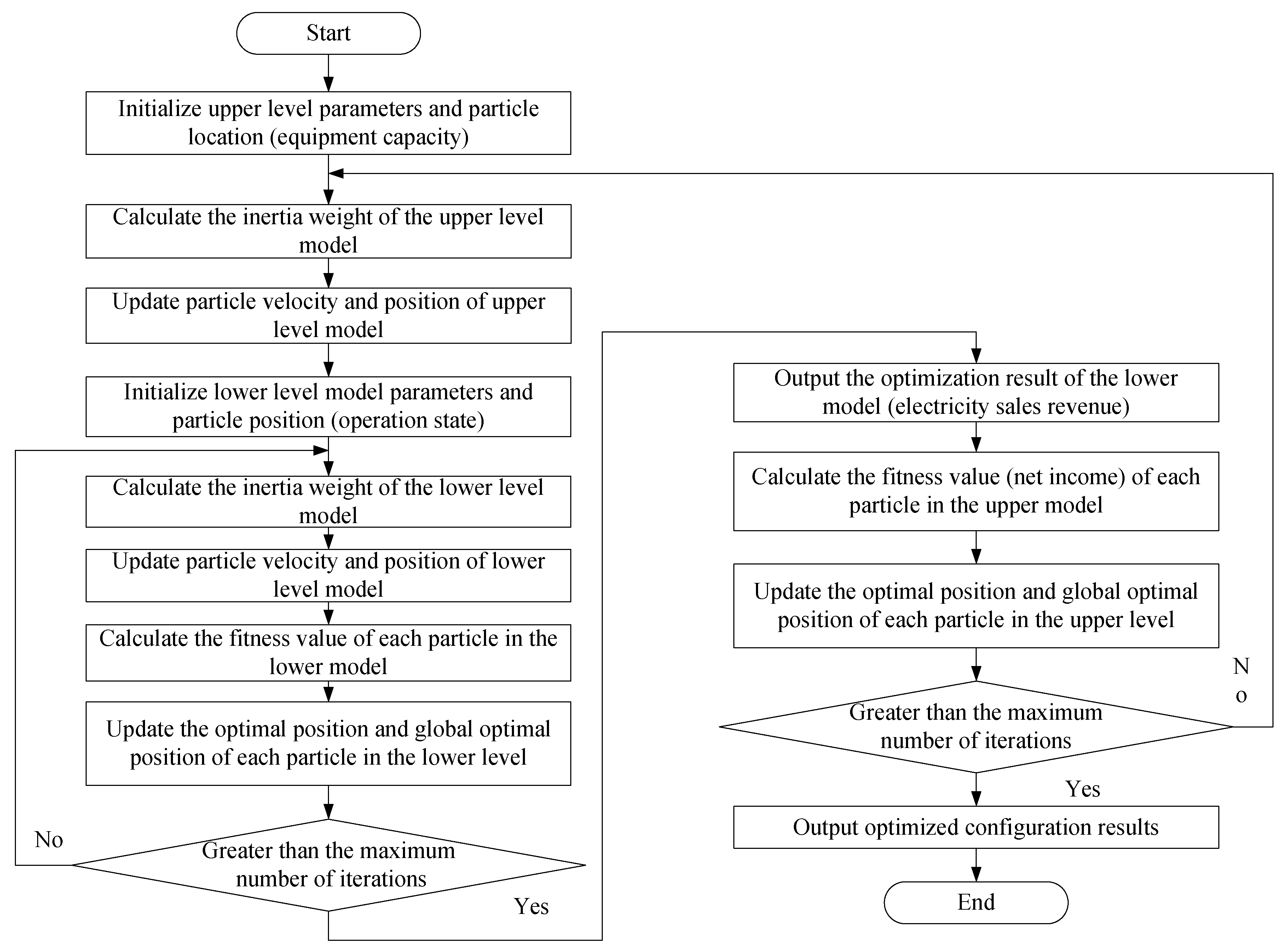
All of the above studies on the planning of WPB-HGS use single-level optimization models. For a WPB-HGS, both equipment capacity and system operating conditions can affect its economy. Equipment capacity determines the cost of equipment purchase and system construction in the initial stage of system construction. The operation and maintenance costs and electricity sales revenue are directly related to the operating status of the system. Therefore, when optimizing the WPB-HGS, it is necessary to consider both the equipment capacity and the operating status. Therefore, this problem is a typical bi-level optimization problem. The upper layer determines the structure of the system and the capacity of the system equipment, and the lower layer optimizes the operating state of the system under the upper-layer equipment capacity configuration results. In Reference [22], a bi-level program was proposed to determine the optimal size of distributed generations and compressed air energy storage (CAES) in an islanded microgrid. In Reference [23], a bi-level model is proposed to optimize the allocation of photovoltaic (PV), wind turbine (WT), and energy storage system (ESS) in distribution networks. At the upper level, a genetic algorithm (GA) is used to optimize the capacity of PV, WT, and ESS. At the lower level, an operation strategy of ESS is proposed first to smooth the power flow. Aiming at capacity optimization of an isolated microgrid, Reference [24] establishes a bi-level capacity optimization model that considers load demand management (LDM) while comprehensively considering load and renewable generation uncertainties.

For a specific project of WPB-HGS, the economic benefit is the most important basis for the investment builder to evaluate the system. However, the existing research often uses a single economic index, such as investment cost or net income, which cannot fully consider the economy of the whole life cycle of WPB-HGS. Therefore, this paper puts the return on investment (ROI) into the optimization objective to improve the system economy. Considering the influence of the operation state of the WPB-HGS on the optimal allocation results, a bi-level model of planning operation integration of the WPB-HGS is established. The effectiveness of the proposed planning model is verified by a case study. At last, it is compared with the single-level planning model to verify that the bi-level planning operation integration model has better economy.

The main contributions of this paper are:

• Established a bi-level model of planning operation integration of the WPB-HGS. This bi-level planning model can optimize the capacity and operation state of the system equipment to improve the economy of planning results.
• Put the return on investment (ROI) into the optimization objective. In consideration of the system revenue, ROI is included in the optimization objective to improve the system economy more comprehensively.
• Compared with the traditional single-level planning model, the integrated bi-level planning operation model is more economical.
• With the increasing application of WPB-HGS, this paper has a certain guiding significance for the optimal configuration design of WPB-HGS in the future.

The remainder of this paper is organized as follows: Section 2 introduces the structure and equipment model of WPB-HGS. Section 3 establishes the double-level programming model of WPB-HGS. Section 4 uses case to verify the proposed model. The concluding remarks are drawn in Section 5.

2. System Description

2.1. Structure of WPB-HGS

The structure of WPB-HGS is shown in Figure 1. The system mainly includes wind turbines (WT), wind turbine converters (WTC), photovoltaic panels (PV), photovoltaic converters (PVC), battery energy storage (BES), battery converters (BC), and other equipment. The DC bus transmits energy to the grid through the grid-connected inverter (GCI). Photovoltaic panels convert solar into electrical energy, which is transmitted to the DC bus after passing through the PVC. The wind turbine converts wind energy into electrical energy, which is transmitted to the DC bus through the WTC.

2.2. System Equipment Model

2.2.1. PV Model

The PV model is as follows [25]:

$$P_{\mathrm{PV}}={\eta }_{\mathrm{PV}}{P}_{\mathrm{stc}}G/G_{stc}\left(1+{\eta }_{\mathrm{T}}\left(T-T_{\mathrm{stc}}\right)\right)$$

(1)

where $P_{\mathrm{PV}}$ is the output power of PV, ${\eta }_{\mathrm{PV}}$ is the generation efficiency of PV, the value is 0.95, $P_{\mathrm{stc}}$ is the output power of PV under standard test conditions, $G$ is the actual light radiation intensity on PV panel, and $G_{stc}$ is the rated light intensity generally taken as 1 kW/m². $T$ is the actual temperature of photovoltaic system, $T_{\mathrm{stc}}$ is standard test temperature, the general value is 25 °C, and ${\eta }_{\mathrm{T}}$ is the power temperature coefficient (%/°C), the general value is −0.47%/°C.

2.2.2. WT Model

The WT model is as follows [26]:

$$\{\begin{array}{cc}{P}_{\mathrm{WT}}=0& v<v_{\mathrm{ci}}\left|\right|v>v_{\mathrm{co}}\\ P_{\mathrm{WT}}=P_{\mathrm{wtr}}\left(v-v_{\mathrm{ci}}\right)/\left(v_{\mathrm{r}}-v_{\mathrm{ci}}\right)& v_{\mathrm{ci}}\le v<v_{\mathrm{r}}\\ P_{\mathrm{WT}}=P_{\mathrm{wtr}}& v_{\mathrm{r}}\le v\le v_{\mathrm{co}}\end{array}$$

(2)

where $P_{\mathrm{WT}}$ is the output power of the WT, $P_{\mathrm{wtr}}$ is the rated output power of the WT, $v_{\mathrm{ci}}$ is the cut-in wind speed of the WT, $v_{\mathrm{co}}$ is the cut-out wind speed, $v_{\mathrm{r}}$ is the rated wind speed, and $v$ is the actual wind speed.

2.2.3. Battery Model

The battery model is as follows:

$$E(t+1)=E(t)+d_{\mathrm{c}}(t){\eta }_{\mathrm{c}}{P}_{\mathrm{c}}(t)\Delta T-d_{\mathrm{d}}(t)\frac{P_{\mathrm{d}}(t)\Delta T}{{\eta }_{\mathrm{d}}}$$

(3)

where $E(t)$ is the remaining energy of the energy storage battery at time t. $d_{\mathrm{c}}(t)$ and $P_{\mathrm{d}}(t)$ are a set of mutually exclusive 0–1 state variables, which respectively represent the charging and discharging states of the energy storage device. Mutually exclusive means that the energy storage device only charges or discharges energy at a certain time. ${\eta }_{\mathrm{c}}$ is the charging efficiency, the value is 0.95. ${\eta }_{\mathrm{d}}$ is the discharging efficiency, the value is 0.95. $P_{\mathrm{c}}(t)$ is the charging power and $P_{\mathrm{d}}(t)$ is the discharging power. The maximum charge and discharge range of the battery is 0.1–1 rated capacity of the battery. If it goes beyond this range, the battery will be damaged.

2.2.4. Battery Life Model

The service life of energy storage battery is not only related to the times of charge and discharge but also the depth of charge and discharge. The number and depth of charge and discharge can be calculated by water flow method. The more charge and discharge times, the greater depth and the shorter service life of the energy storage battery. The battery life model is as follows [27]:

$$T_{\mathrm{b}}=0.2/{\displaystyle \sum _{i=1}^n(1-e^{-\frac{1}{k_{\delta 1}{\delta }_n{}^{k_{\delta 2}}+k_{\delta 3}}})}$$

(4)

where $T_{\mathrm{b}}$ is the energy storage battery service life (year); n is the number of charging and discharging of the energy storage battery;${\delta }_n$ is the charge and discharge depth; and $k_{\delta 1}$ (1.4 × 10⁵), $k_{\delta 2}$ (−0.501), and $k_{\delta 3}$ (−1.23 × 10⁵) are charge-discharge depth loss coefficients.

3. Bi-Level Planning Model

There are two main factors that affect the economic index of the WPB-HGS, one is the investment cost of the system and the other is the income from the sale of electricity. Investment cost mainly refers to the cost of energy supply and energy storage equipment, which is mainly related to equipment capacity. The larger the equipment capacity is, the greater the investment cost is. The income from selling electricity in WPB-HGS is directly related to the operation status of the system. The output power of each equipment determines the output power of the system, and thus the income from selling electricity. The traditional single-level optimization model cannot optimize the equipment capacity and operation state at the same time. Based on this, this paper constructs a bi-level planning model of equipment capacity of WPB-HGS. The basic workflow is shown in Figure 2. The upper-level model takes the maximum annual net income and ROI as the goal to optimize the equipment capacity of the WPB-HGS. The device capacity configuration results are brought into the lower-level model as constraints. The lower-level model optimizes the operation state of the system with the goal of the highest proceed from the sale of electricity and obtains the proceed from the sale of electricity. The proceeds from the sale of electricity are then transferred to the upper level to calculate the net revenues and ROI of the system. After several iterations of the upper- and lower-level models, the optimal capacity allocation results are obtained.

3.1. Upper-Level Model

The upper-level model allocates the equipment capacity with the goal of the maximum annual net income and the maximum ROI.

3.1.1. Annual Net Income

The annual net income objective function is as follows:

$$\max f_1=C_{\mathrm{M}}-(C_{\mathrm{INV}}+C_{\mathrm{OP}})$$

(5)

where $C_{\mathrm{M}}$ is the total annual revenue from the sale of electricity, $C_{\mathrm{INV}}$ is the annual value of equipment investment cost, and $C_{\mathrm{OP}}$ is the annual operation and maintenance cost.

The total annual revenue from the sale of electricity is as follows:

$$C_{\mathrm{M}}=365C_{\mathrm{mond}}$$

(6)

where $C_{\mathrm{mond}}$ is the daily electricity sales revenue of the system, and it is the optimization result of the lower-level operation optimization model.

The annual value of equipment investment cost model is as follows:

$$C_{\mathrm{INI}}=\left(\begin{array}{c}(m_{\mathrm{pv}}{N}_{\mathrm{pv}}+m_{\mathrm{wt}}{N}_{\mathrm{wt}})+\hfill \\ {\displaystyle \sum _{i=1}^n\left(m_{\mathrm{g}}^i{N}_{\mathrm{g}}^i+m_{\mathrm{g}}^i{N}_{\mathrm{g},\mathrm{r}}^i\right)}+\hfill \\ m_{\mathrm{s}}{C}_{\mathrm{s}}+m_{\mathrm{s}}{C}_{\mathrm{s},\mathrm{r}}\end{array}\right)\frac{r_0{\left(1+r_0\right)}^{Y_{\mathrm{y}}}}{r_0{\left(1+r_0\right)}^{Y_{\mathrm{y}}}-1}$$

(7)

where $m_{\mathrm{pv}}$ and $m_{\mathrm{wt}}$ are the individual prices of PV and WT; $N_{\mathrm{pv}}$ and $N_{\mathrm{wt}}$ are the number of PV and WT; since the service life of PV panel and WT are assumed to be the whole project cycle, there are no replacement capacity; $m_{\mathrm{g}}^i$ represents the unit price of converter. According to the structure diagram of WPB-HGS shown in Figure 1, it can be seen that there are four types of converters in total, namely: energy storage converter, photovoltaic converter, wind turbine converter, and bidirectional DC/AC converter; $N_{\mathrm{g}}^i$ represents the quantity of type i converter; $N_{\mathrm{g},\mathrm{r}}^i$ represents the replacement quantity of type i converter; $m_{\mathrm{s}}$ is the unit price of energy storage battery, $C_{\mathrm{s}}$ is the capacity of energy storage battery; $C_{\mathrm{s},\mathrm{r}}$ is the replacement capacity of energy storage battery; $r_0$ is the discount rate; $Y_{\mathrm{y}}$ is the project cycle.

The annual maintenance cost model is as follows:

$$C_{\mathrm{OP}}=K_{\mathrm{OP}}{C}_{\mathrm{INI}}$$

(8)

where $K_{\mathrm{OP}}$ is the annual maintenance cost factor.

3.1.2. ROI

Return on investment refers to the economic return investors get from investment activity. As an important economic index, the ROI can reflect the comprehensive profitability of investment projects. Moreover, ROI eliminates the incomparable factors of profit difference caused by different investment amounts, so it has horizontal comparability that is helpful to judge the profit of each investment project. Therefore, this paper proposes to add the ROI to the optimization target of optimal capacity allocation of WPB-HGS to improve the economy of allocation results.

The ROI objective function is as follows:

$$\max f_2=\frac{C_{\mathrm{M}}}{C_{\mathrm{TOTAL}}}\times 100\%$$

(9)

where $C_{\mathrm{M}}$ is the total income from the annual electricity sales, and $C_{\mathrm{TOTAL}}$ is the total investment cost of the system.

3.1.3. The Treatment of the Upper Optimization Targets

In this paper, each optimization objective is normalized, weighted, and combined into a comprehensive optimization objective. The comprehensive optimization objective is as follows:

$$\max F_1={\omega }_1\left|\frac{f_1-f_1^{\min }}{f_1^{\max }-f_1^{\min }}\right|+{\omega }_2\left|\frac{f_2-f_2^{\min }}{f_2^{\max }-f_2^{\min }}\right|$$

(10)

where $f_1^{\max }$ and $f_1^{\min }$ are the ideal maximum and minimum values of objective function $f_1$, $f_2^{\max }$ and $f_2^{\min }$ are the ideal maximum and minimum values of objective function $f_2$, and ${\omega }_1$ and ${\omega }_2$ represent the weight coefficients of each sub-objective function.

3.2. Lower-Level Model

3.2.1. Optimization Objective

The lower-level optimization model optimizes the operation state of the system with the goal of maximizing the daily electricity sales revenue of the WPB-HGS. The optimization objective is as follows:

$$\max F_2=C_{\mathrm{mond}}$$

(11)

where $C_{\mathrm{mond}}$ is the daily electricity sales revenue of the system. The detail is as follows:

$$C_{\mathrm{mond}}={\displaystyle \sum _{t=1}^{T}f(P_{\mathrm{out}}(t))}$$

(12)

where $P_{\mathrm{out}}(t)$ is the output power of the system. $f(*)$ is a function of the revenue from electricity sales.

3.2.2. Constraint Condition

(1) Power balance constraint

The power balance constraint is as follows:

$$P_{\mathrm{out}}(t)=P_{\mathrm{pv}}(t)+P_{\mathrm{wt}}(t)-P_{\mathrm{bat}}(t)$$

(13)

where $P_{\mathrm{out}}(t)$ is the system grid connected output power, $P_{\mathrm{pv}}(t)$ is the PV output power, $P_{\mathrm{wt}}(t)$ is the wind turbine output power, and $P_{\mathrm{bat}}(t)$ is the energy storage battery absorption power.

(2) Output constraint of distributed generation

The output constraint of PV and WT are as follow:

$$P_{\mathrm{pv}}^{\min }(t)\le P_{\mathrm{pv}}(t)\le P_{\mathrm{pv}}^{\max }(t)$$

(14)

$$P_{\mathrm{wt}}^{\min }(t)\le P_{\mathrm{wt}}(t)\le P_{\mathrm{wt}}^{\max }(t)$$

(15)

where $P_{\mathrm{pv}}(t)$ and $P_{\mathrm{wt}}(t)$ are the output power of PV and WT, $P_{\mathrm{pv}}^{\min }(t)$ and $P_{\mathrm{pv}}^{\max }(t)$ are the minimum and maximum allowable output power of PV, and $P_{\mathrm{wt}}^{\min }(t)$ and $P_{\mathrm{wt}}^{\max }(t)$ are the minimum and maximum allowable output values of WT.

(3) Output constraint of converter equipment

The output constraint of converter equipment is as follows:

$$P_{\mathrm{g}}^{i,\min }(t)\le P_g^i(t)\le P_{\mathrm{g}}^{i,\max }(t)$$

(16)

where $P_g^i(t)$ is the output power of converter and $P_{\mathrm{g}}^{i,\min }$ and $P_{\mathrm{g}}^{i,\max }(t)$ are the minimum and maximum allowable output power of converter.

(4) Battery charging and discharging power constraints

The output constraints of PV and WT are as follow:

$${\eta }_{\mathrm{d}}{P}_{\mathrm{d}}^{\min }\le P_{\mathrm{d}}(t)\le {\eta }_{\mathrm{d}}{P}_{\mathrm{d}}^{\max }$$

(17)

$${\eta }_{\mathrm{c}}{P}_{\mathrm{c}}^{\min }\le P_{\mathrm{c}}(t)\le {\eta }_{\mathrm{c}}{P}_{\mathrm{c}}^{\max }$$

(18)

where $P_{\mathrm{d}}(t)$ and $P_{\mathrm{c}}(t)$ are the discharge and charging power of the energy storage battery, ${\eta }_{\mathrm{d}}$ and ${\eta }_{\mathrm{c}}$ are the discharge efficiency and charging efficiency, $P_{\mathrm{d}}^{\min }$ and $P_{\mathrm{d}}^{\max }$ are the minimum power and maximum power allowed by discharge, and $P_{\mathrm{c}}^{\min }$ and $P_{\mathrm{c}}^{\max }$ are the minimum power and maximum power allowed by charging.

(5) Battery state constraints

The battery state constraints are as follow:

$$S(t+1)=S(t)+\frac{d_{\mathrm{c}}(t){\eta }_{\mathrm{c}}{P}_{\mathrm{c}}(t)\Delta T}{C_{\mathrm{bat}}}-\frac{d_{\mathrm{d}}(t)P_{\mathrm{d}}(t)\Delta T}{{\eta }_{\mathrm{d}}{C}_{\mathrm{bat}}}$$

(19)

$$S_{\min }\le S(t)\le S_{\max }$$

(20)

$$S(0)=S(T)$$

(21)

where $S(t)$ is the state of charge (SOC) of the battery; $d_{\mathrm{c}}(t)$ and $d_{\mathrm{d}}(t)$ are a set of mutually exclusive 0–1 state variables, respectively, representing the charging and discharging state of the battery. Mutually exclusive means that the battery can only charge or discharge energy at the same time. ${\eta }_{\mathrm{c}}$ represents the charging efficiency, ${\eta }_{\mathrm{d}}$ represents the discharging efficiency, $P_{\mathrm{c}}(t)$ represents the charging power, and $P_{\mathrm{d}}(t)$ represents the discharging power. $C_{\mathrm{bat}}$ is the capacity of battery, $S_{\min }$ is the minimum allowable SOC of battery, and $S_{\max }$ is the maximum allowable SOC of battery. Equation (21) shows that the SOC of the battery should be equal before and after a whole scheduling cycle.

(6) Output power fluctuation constraint

The output power fluctuation constraint is as follows:

$$\left|P_{\mathrm{out}}(t)-P_{\mathrm{out}}(t-1)\right|<P_{\lim }$$

(22)

where $P_{\mathrm{out}}(t)$ is the system output power at time t, $P_{\mathrm{out}}(t-1)$ is the system output power at time t − 1, and $P_{\lim }$ is the maximum fluctuation power.

3.3. Solution of the Model

Generally, the algorithms used to solve the optimal configuration model can be divided into two categories: mathematical programming method and intelligent algorithm. Although the mathematical programming method is simple in calculation, its accuracy is low. Although the common genetic algorithm has high precision, it has a complex structure and a large amount of calculation, so its convergence speed is slow. As a kind of bionic intelligent algorithm, particle swarm optimization (PSO) algorithm has the advantages of fast convergence speed and less adjustable parameters. Because of its simple structure, it is conducive to engineering realization. In this paper, adaptive weight particle swarm optimization (AW-PSO) is used to solve the bi-level planning model. Compared with the PSO, the AW-PSO has higher search accuracy and can avoid falling into the local optimal solution. The model solving process based on AW-PSO is shown in Figure 3.

4. Case Study

4.1. Basic Data

In order to verify the effectiveness of the proposed planning scheme, the actual engineering data is selected for simulation. The structure of the whole system is shown in Figure 1. Typical daily data of solar radiation intensity, wind speed, and temperature are shown in Figure 4, Figure 5, and Figure 6, respectively. All typical daily data are from renewable energy power generation system projects. The system dispatching time is 1 min, the dispatching cycle is 1 day, and the system output fluctuation before and after the unit dispatching time is limited to 120 kW.

The device parameters of the system are shown in

Table 1. The device parameters of the system.

Name	Unit Capacity (kW)	Unit Cost ($)	Most Common Service Life (Year)
PV	1	800	25
WT	500	500,000	25
BC	300	12,000	10
PVC	50	2000	10
WTC	500	20,000	10
GCI	1000	40,000	10

.

The battery parameters are shown in

Table 2. The battery parameters.

Name	Unit Capacity Cost ($/kWh)	SOC Range	Most Common Service Life (Year)
Battery	300	[0.1, 1]	10

.

4.2. Billing Strategy for Electricity Sales

In this example, all the power generated by the system is sold to the grid. The peak time is 9–22 points every day, and the off-peak time is 0–8 points and 23–24 points. The unit billing time is 15 min. The guaranteed energy at the peak time (GE_p) is 3000 kWh/15 min. The guaranteed energy at the off-peak time is 2000 kWh/15 min. The peak time and the off-peak time (GE_np) are charged according to different electricity sales rules. The price parameters are shown in

Table 3. Electricity price.

Name	Price ($/kWh)
Basic electricity price (BEP)	0.1
Penalty price (PP)	0.01

.

The rules for selling electricity at peak time are shown in

Table 4. The rules for selling electricity at peak time.

Grid Connected Power	Proceeds From Sale of Electricity
$E(t)<80\%G{E}_{\mathrm{p}}$	$BEP\ast E(t)-PP(0.8G{E}_{\mathrm{p}}-E(t))$
$80\%G{E}_{\mathrm{p}}\le E(t)<100\%G{E}_{\mathrm{p}}$	$BEP\ast E(t)$
$100\%G{E}_{\mathrm{p}}\le E(t)<110\%G{E}_{\mathrm{p}}$	$BEP\ast G{E}_{\mathrm{p}}+0.5BEP(E(t)-G{E}_{\mathrm{p}})$
$E(t)\ge 110\%G{E}_{\mathrm{p}}$	$BEP\ast G{E}_{\mathrm{p}}+0.5BEP\ast 0.1G{E}_{\mathrm{p}}$

.

In Table 4, $E(t)$ is the output electric energy in unit time period, and $G{E}_{\mathrm{p}}$ is the guaranteed energy in peak time. In peak time, when $E(t)$ is less than 80%$G{E}_{\mathrm{p}}$, the output power will be sold according to the basic price, and the part less than 80%$G{E}_{\mathrm{p}}$ will be fined accordingly. When $E(t)$ is more than 80%$G{E}_{\mathrm{p}}$ and less than 100%$G{E}_{\mathrm{p}}$, all electric energy will be charged according to the basic price. When $E(t)$ is more than 100%$G{E}_{\mathrm{p}}$ and less than 110%$G{E}_{\mathrm{p}}$, the part of 100% $G{E}_{\mathrm{p}}$ will sell electricity according to the basic price, and the part between 100% and 110% $G{E}_{\mathrm{p}}$ will be sold according to 50% of the basic price. When $E(t)$ is more than 110% $G{E}_{\mathrm{p}}$, the part higher than 110% $G{E}_{\mathrm{p}}$ will not be calculated as power sale income.

The rules for selling electricity at off-peak time are shown in

Table 5. The rules for selling electricity at off-peak time.

Grid Connected Power	Proceeds From Sale of Electricity
$E(t)<100\%G{E}_{\mathrm{np}}$	$BEP\ast E(t)$
$100\%G{E}_{\mathrm{np}}\le E(t)<110\%G{E}_{\mathrm{np}}$	$BEP\ast G{E}_{\mathrm{p}}+0.5BEP(E(t)-G{E}_{\mathrm{p}})$
$E(t)\ge 110\%G{E}_{\mathrm{p}}$	$BEP\ast G{E}_{\mathrm{np}}+0.5BEP\ast 0.1G{E}_{\mathrm{np}}$

.

In Table 5, $E(t)$ is the output electric energy in unit time period, and $G{E}_{\mathrm{np}}$ is the guaranteed energy in off-peak time. In off-peak time, when $E(t)$ is less than 100% $G{E}_{\mathrm{np}}$, all electric energy will be charged according to the basic price. When $E(t)$ is more than 100%$G{E}_{\mathrm{np}}$ and less than 110%$G{E}_{\mathrm{np}}$, the part of 100%$G{E}_{\mathrm{np}}$ will sell electricity according to the basic price, and the part between 100% and 110%$G{E}_{\mathrm{np}}$ will be sold according to 50% of the basic price. When $E(t)$ is more than 110%$G{E}_{\mathrm{np}}$, the part higher than 110%$G{E}_{\mathrm{np}}$ will not be calculated as power sale income.

4.3. Scene Design

In order to study the impact of ROI optimization goals on planning, two scenarios were set up for comparative analysis. The specific scenarios are as follows:

Scenario 1: Only plan the capacity of WPB-HGS with the goal of maximum annual net income.

Scenario 2: Plan the capacity of WPB-HGS with the goal of combining annual net income and ROI as the goal.

4.4. Results and Discussion

Based on the bi-level planning model established in this paper, the typical data of scenery in Figure 4 and Figure 5, the basic parameters of each equipment in Table 1 and Table 2, and the electricity sales strategy in Table 4 and Table 5, AW-PSO was used to solve the model. The device configuration results are shown in

Table 6. Configuration results.

Device	Scenario 1	Scenario 2
PV (kW)	5763	7282
WT (kW)	27,500	23,000
Battery(kWh)	2805	2249
BC (kW)	6000	5400
PVC (kW)	5800	7300
WTC (kW)	27,500	23,000
GCI (kW)	18,000	17,000

.

According to Table 6, considering ROI, the PV capacity increases from 5763 kW to 7282 kW, with an increase of 1519 kW. The capacity of WT is reduced from 27,500 kW to 23,000 kW, a decrease of 4500 kW. The reduction of the total capacity of PV and WT reduces the system output fluctuation, thereby reducing the energy storage battery capacity. Therefore, the energy storage battery capacity is reduced from 2805 kWh to 2249 kWh, which is reduced by 556 kWh. No matter in scenario 1 or scenario 2, compared with PV, WT capacity is obviously higher, because the wind can be used for a long time throughout the day. According to the typical day data of the scenery in Figure 4 and Figure 5, the light resources only exist during the day, and increase with time and then decrease, with uneven distribution. The wind resources can be used no matter day or night, and the distribution is relatively uniform, so the WT with a larger capacity can use renewable resources more reasonably and effectively improve the equipment utilization efficiency.

The economic indicators of the system in each scenario are shown in

Table 7. Economic index.

Economic Index	Scenario 1	Scenario 2
Annual net income (106$)	6.8623	6.8028
Annual cost (106$)	2.2381	1.8987
ROI	0.1626	0.1833
Investment payback period (year)	6.2	5.4
Total cost (107$)	5.5953	4.7469
Total revenue (108$)	1.7155	1.7007

.

It can be seen from Table 7 that after considering ROI in scenario 2, the total cost decreased from 5.5953 × 10⁷ $ to 4.7469 × 10⁷ $, a decrease of 15.16%. The ROI increased from 0.1626 to 0.1833, an increase of 12.73%; The investment recovery period has also been shortened from 6.2 years to 5.4 years. However, the overall benefits of the system remain substantially unchanged, decreased from 1.7155 × 10⁸ $ to 1.7007 × 10⁸$, down only 0.86%.

According to the comparison results in Table 7 that compared with not considering ROI, after adding ROI to the optimization goal, it can effectively reduce the total investment cost of the system, increase the project ROI, and reduce the investment recovery period, while ensuring that the total system revenue is reduced by a very small percentage.

The cost and distribution of each device of the system in the two scenarios are shown in Figure 7 and Figure 8.

It can be seen from the combination of Figure 7 and Figure 8 that among all devices, the cost of WT accounts for the largest proportion of the cost of all devices, which is 59% and 58% in two scenarios. The second is energy storage batteries, which are 24% and 22%. Again, it is PV equipment, which accounts for 10% and 14% in the two scenarios, respectively. The smallest percentage is GCI. Although the energy storage battery capacity is lower than the capacity of PV equipment, its equipment cost accounted for more than PV equipment. This is because the service life of PV equipment is the entire project cycle, and there is no replacement cost. The service life of energy storage battery is related to the depth and frequency of charge and discharge. After many charging and discharging processes, the service life of the battery is greatly reduced, resulting in the need to replace the energy storage battery multiple times throughout the project cycle, thereby increasing the total cost of the energy storage battery.

Figure 9 is the output curve of each device of the system in scenario 2.

At 0–7 o’clock, the wind resource is sufficient and the light radiation intensity is 0. At this time, the system output is provided by the WT. At 7–19 o’clock, the wind speed decreased and the output of WT was insufficient, while the PV output increased with the increase of light radiation intensity. After 19 o’clock, the light radiation intensity will be 0 and the wind speed will increase. At this time, the system output will be provided by WT.

It can be seen from the output curve in Figure 9 that the output of WT and PV have good complementary characteristics.

It can be seen from the energy storage output curve in Figure 9 that the energy storage battery output has been fluctuating up and down at 0, and has not played the role of peak shaving and valley filling. This is because the investment cost and replacement cost of energy storage batteries are high, and the use of energy storage batteries for peak output and valley filling in system output is not economical. Therefore, the main function of the energy storage battery is to smooth the output of the system. At 7–19 o’clock, the energy storage battery is charged and discharged relatively frequently and the power is relatively high. This is because the superposition of the WT and PV output causes the system output fluctuation to become larger. The energy storage battery needs to be frequently charged and discharged to smooth the system output.

In scenario 2, the output curve of the system before and after stabilizing the fluctuation by the energy storage battery is shown in Figure 10.

Table 8. Maximum fluctuation of system output.

Name	Before Stabilizing the Fluctuation	After Stabilizing the Fluctuation
Maximum power fluctuation (kW)	5590	120

shows the maximum power difference in system output before and after unit time.

According to Figure 10 and Table 8, the maximum output fluctuation of the system per unit time is 5590 kW before the energy storage battery stabilizes the fluctuation. The maximum output fluctuation per unit time of the system is 120 kW after the energy storage battery stabilizes the fluctuation. This meets the requirements of maximum fluctuation power. The energy storage battery plays a good role in stabilizing the fluctuation.

SOC of energy storage battery is shown in Figure 11. According to Figure 9 and Figure 10, due to the large fluctuation of WT and PV output, the energy storage battery needs to conduct high-frequency charging and discharging to ensure the stability of output power, resulting in high frequency and large fluctuation of energy storage state.

4.5. Verification of Bi-Level Planning Model

In order to verify the effectiveness of the proposed bi-level planning model, it is compared with the traditional single-level planning model. The single-layer planning model adopted only plans of the system equipment capacity and does not consider the system operation state. Compared with the bi-level planning model, the single-level planning model also sets up two scenarios for comparative analysis. The specific scenarios are as follows:

Scenario 3: Based on the single-level programming model, only plan the capacity of WPB-HGS with the goal of maximum annual net income.

Scenario 4: Based on the single-level programming model, plan the capacity of WPB-HGS with the goal of combining annual net income and ROI as the goal.

The single-level planning model is solved, and the equipment configuration results are shown in

Table 9. Configuration results (single-level model).

Device	Scenario 3	Scenario 4
PV (kW)	5692	6972
WT (kW)	27,500	23,000
Battery(kWh)	2628	3260
BC (kW)	6900	5100
PVC (kW)	5700	7000
WTC (kW)	27,500	23,000
GCI (kW)	17,000	15,000

.

The economic indicators of the system in each scenario are shown in

Table 10. Economic index (single-level model).

Economic Index	Scenario 1	Scenario 2
Annual net income (106$)	6.6500	6.6259
Annual cost (106$)	2.1314	1.8937
ROI	0.1648	0.1800
Investment payback period (year)	6.1	5.5
Total cost (107$)	5.3285	4.7344
Total revenue (108$)	1.6625	1.6564

.

According to the analysis of the economic indicators of the system under the single-level planning model in Table 10, after considering the ROI in the optimization objective of scenario 4, the total cost of the system is reduced by 11.14%; the ROI is increased by 9.23%; the payback period is also shortened from 6.1 years to 5.5 years; however, the total return of the system is basically unchanged, only reduced by 0.36%.

This shows that, like the bi-level planning model, when the ROI is added to the optimization objective of the single-level planning model, it can effectively reduce the total investment cost of the system and improve the ROI of the project, to improve the overall economy, while ensuring the reduction of the minimum proportion of the total return on investment of the system.

The total income of single-level and bi-level planning models in different scenarios are shown in

Table 11. Total income.

Scene	Optimization Model	Total Income (108$)
Scenario 1	Bi-level (No ROI)	1.7155
Scenario 2	Bi-level (Consider ROI)	1.7007
Scenario 3	Single-level (No ROI)	1.6625
Scenario 4	Single-level (Consider ROI)	1.6564

.

It can be seen from Table 11 that when ROI is not considered in the optimization objective, the total income of the single-level planning model is 5.3 × 10⁶$ lower than that of the bi-level planning model. When ROI is considered in the optimization objective, the total income of single-level planning model is 4.4 × 10⁶$ lower than that of bi-level planning model.

Therefore, compared with the single-level planning model, the bi-level planning model is more economical.

5. Conclusions

In order to consider the economy of the planning results of WPB-HGS more comprehensively, this paper proposes a method of optimal allocation of WPB-HGS considering the ROI. The effectiveness of the proposed method is verified by a typical example, and the results of optimal configuration and operation are analyzed. At the same time, the paper compares the bi-level planning model with the single-level planning model. The results show that when planning the equipment capacity of WPB-HGS, considering the ROI in the optimization objective, the investment cost of the system can be reduced while the total return is basically unchanged, to improve the return on investment and shorten the investment return period. Compared with the traditional single-level planning model, the bi-level planning model proposed in this paper is more economical.

References

1. Guo, Y.; Gao, H.; Wu, Z. Hybrid wind-PV system capacity limit calculation of based on constraint transformer. In Proceedings of the 2016 China International Conference on Electricity Distribution (CICED), Xi’an, China, 10–13 August 2016; pp. 1–5. [Google Scholar]
2. Nurunnabi, M.; Roy, N.K.; Hossain, E.; Pota, H.R. Size Optimization and Sensitivity Analysis of Hybrid Wind/PV Micro-Grids- A Case Study for Bangladesh. IEEE Access 2019, 7, 150120–150140. [Google Scholar] [CrossRef]
3. Feng, J.; Zeng, B.; Zhao, D.; Wu, G.; Liu, Z.; Zhang, J. Evaluating Demand Response Impacts on Capacity Credit of Renewable Distributed Generation in Smart Distribution Systems. IEEE Access 2018, 6, 14307–14317. [Google Scholar] [CrossRef]
4. Li, Y.; Chi, Y.; Wang, X.; Tian, X.; Jianqing, J. Practices and Challenge on Planning with Large-scale Renewable Energy Grid Integration. In Proceedings of the 2019 IEEE 3rd Conference on Energy Internet and Energy System Integration (EI2), Changsha, China, 8–10 November 2019; pp. 118–121. [Google Scholar]
5. Savkin, A.V.; Khalid, M.; Agelidis, V. A Constrained Monotonic Charging/Discharging Strategy for Optimal Capacity of Battery Energy Storage Supporting Wind Farms. IEEE Trans. Sustain. Energy 2016, 7, 1224–1231. [Google Scholar] [CrossRef]
6. Lin, L.; Li, L.; Jia, L. An optimal capacity configuration method of wind/PV and energy storage co-generation system. In Proceedings of the 2014 IEEE PES General Meeting | Conference & Exposition, National Harbor, MD, USA, 27–31 July 2014; pp. 1–5. [Google Scholar]
7. Chen, X.; Leung, K.-C.; Lam, A.Y. Power Output Smoothing for Renewable Energy System: Planning, Algorithms, and Analysis. IEEE Syst. J. 2020, 14, 1034–1045. [Google Scholar] [CrossRef]
8. Long, H.; Eghlimi, M.; Zhang, Z. Configuration Optimization and Analysis of a Large Scale PV/Wind System. IEEE Trans. Sustain. Energy 2016, 8, 84–93. [Google Scholar] [CrossRef]
9. Wu, X.; Xu, K.; Wang, Z.; Gong, Y. Optimized capacity configuration of an integrated power system of wind, photovoltaic and energy storage device based on improved particle swarm optimizer. In Proceedings of the 2017 IEEE Conference on Energy Internet and Energy System Integration (EI2), Beijing, China, 27–28 November 2017; pp. 1–6. [Google Scholar]
10. Li, P.; Dargaville, R.; Liu, F.; Xia, J.; Song, Y.-D. Data-Based Statistical Property Analyzing and Storage Sizing for Hybrid Renewable Energy Systems. IEEE Trans. Ind. Electron. 2015, 62, 6996–7008. [Google Scholar] [CrossRef]
11. Yang, P.; Nehorai, A. Joint Optimization of Hybrid Energy Storage and Generation Capacity with Renewable Energy. IEEE Trans. Smart Grid 2014, 5, 1566–1574. [Google Scholar] [CrossRef]
12. Shadmand, M.B.; Balog, R. Multi-Objective Optimization and Design of Photovoltaic-Wind Hybrid System for Community Smart DC Microgrid. IEEE Trans. Smart Grid 2014, 5, 2635–2643. [Google Scholar] [CrossRef]
13. Ke, B.R.; Ku, T.T.; Ke, Y.L.; Chuang, C.Y.; Chen, H.Z. Sizing the Battery Energy Storage System on a University Campus with Prediction of Load and Photovoltaic Generation. IEEE Trans. Ind. Appl. 2015, 52, 1136–1147. [Google Scholar]
14. Moreira, A.; Pozo, D.; Street, A.; Sauma, E. Reliable Renewable Generation and Transmission Expansion Planning: Co-Optimizing System’s Resources for Meeting Renewable Targets. IEEE Trans. Power Syst. 2016, 32, 3246–3257. [Google Scholar] [CrossRef]
15. Sheng, S.; Zhang, J. Capacity configuration optimisation for stand-alone micro-grid based on an improved binary bat algorithm. J. Eng. 2017, 2017, 2083–2087. [Google Scholar] [CrossRef]
16. Silva, A.R.; Estanqueiro, A. Optimal Planning of Isolated Power Systems with near 100% of Renewable Energy. IEEE Trans. Power Syst. 2020, 35, 1274–1283. [Google Scholar] [CrossRef]
17. Kaur, R.; Krishnasamy, V.; Kandasamy, N.K.; Kumar, S. Discrete Multiobjective Grey Wolf Algorithm Based Optimal Sizing and Sensitivity Analysis of PV-Wind-Battery System for Rural Telecom Towers. IEEE Syst. J. 2020, 14, 729–737. [Google Scholar] [CrossRef]
18. Qiu, J.; Xu, Z.; Zheng, Y.; Wang, N.; Dong, Z.Y. Distributed generation and energy storage system planning for a distribution system operator. IET Renew. Power Gener. 2018, 12, 1345–1353. [Google Scholar] [CrossRef]
19. Zeng, B.; Zhang, J.; Yang, X.; Wang, J.; Dong, J.; Zhang, Y. Integrated Planning for Transition to Low-Carbon Distribution System With Renewable Energy Generation and Demand Response. IEEE Trans. Power Syst. 2013, 29, 1153–1165. [Google Scholar] [CrossRef]
20. Akram, U.; Khalid, M.; Shafiq, S. An Innovative Hybrid Wind-Solar and Battery-Supercapacitor Microgrid System—Development and Optimization. IEEE Access 2017, 5, 25897–25912. [Google Scholar] [CrossRef]
21. Akram, U.; Khalid, M.; Shafiq, S. Optimal sizing of a wind/solar/battery hybrid grid-connected microgrid system. IET Renew. Power Gener. 2018, 12, 72–80. [Google Scholar] [CrossRef]
22. Zhang, J.; Li, K.J.; Wang, M.; Lee, W.J.; Gao, H.; Zhang, C.; Li, K. A Bi-Level Program for the Planning of an Islanded Microgrid Including CAES. IEEE Trans. Ind. Appl. 2016, 52, 2768–2777. [Google Scholar] [CrossRef]
23. Liu, Y.; Yang, J.; Zhu, X.; Wang, Y.; He, B.; Zhu, J.; Chen, Y. Bi-level planning model for optimal allocation of WT–PV–ESS in distribution networks. J. Eng. 2017, 2017, 1696–1701. [Google Scholar] [CrossRef]
24. Ma, G.; Cai, Z.; Xie, P.; Liu, P.; Xiang, S.; Sun, Y.; Guo, C.; Dai, G. A Bi-Level Capacity Optimization of an Isolated Microgrid with Load Demand Management Considering Load and Renewable Generation Uncertainties. IEEE Access 2019, 7, 83074–83087. [Google Scholar] [CrossRef]
25. Moshi, G.G.; Bovo, C.; Berizzi, A.; Gladson, M.G. Optimal operational planning for PV-Wind-Diesel-battery microgrid. In Proceedings of the 2015 IEEE Eindhoven PowerTech, Eindhoven, The Netherlands, 29 June–2 July 2015; pp. 1–6. [Google Scholar]
26. Yuan, X.; Yang, F.; Xu, J.; Liu, H. Configuration Optimization of Wind-Solar-Storage System considering Demand Response. In Proceedings of the 2018 5th International Conference on Electric Power and Energy Conversion Systems (EPECS), Kitakyushu, Japan, 23–25 April 2018; pp. 1–6. [Google Scholar]
27. Xu, B.; Oudalov, A.; Ulbig, A.; Andersson, G.; Kirschen, D.S. Modeling of Lithium-Ion Battery Degradation for Cell Life Assessment. IEEE Trans. Smart Grid 2016, 9, 1131–1140. [Google Scholar] [CrossRef]
Figure 1. Structure of wind-photovoltaic-battery hybrid generation system (WPB-HGS).
Energies 13 03046 g001
Figure 2. Bi-level planning flowchart.
Energies 13 03046 g002
Figure 3. Model solution flowchart.
Energies 13 03046 g003
Figure 4. Typical solar radiation intensity.
Energies 13 03046 g004
Figure 5. Typical wind speed.
Energies 13 03046 g005
Figure 6. Typical temperature.
Energies 13 03046 g006
Figure 7. Cost of equipment in different scenarios.
Energies 13 03046 g007
Figure 8. Cost distribution of each equipment.
Energies 13 03046 g008
Figure 9. Output of equipment in scenario 2.
Energies 13 03046 g009
Figure 10. System output before and after stabilizing fluctuation in scenario 2.
Energies 13 03046 g010
Figure 11. State of charge (SOC) of energy storage battery in scenario 2.
Energies 13 03046 g011