An Assessment of Onshore and Offshore Wind Energy Potential in India Using Moth Flame Optimization

Abstract

Wind energy is one of the supremely renewable energy sources and has been widely established worldwide. Due to strong seasonal variations in the wind resource, accurate predictions of wind resource assessment and appropriate wind speed distribution models (for any location) are the significant facets for planning and commissioning wind farms. In this work, the wind characteristics and wind potential assessment of onshore, offshore, and nearshore locations of India—particularly Kayathar in Tamilnadu, the Gulf of Khambhat, and Jafrabad in Gujarat—are statistically analyzed with wind distribution methods. Further, the resource assessments are carried out using Weibull, Rayleigh, gamma, Nakagami, generalized extreme value (GEV), lognormal, inverse Gaussian, Rician, Birnbaum–Sandras, and Bimodal–Weibull distribution methods. Additionally, the advent of artificial intelligence and soft computing techniques with the moth flame optimization (MFO) method leads to superior results in solving complex problems and parameter estimations. The data analytics are carried out in the MATLAB platform, with in-house coding developed for MFO parameters estimated through optimization and other wind distribution parameters using the maximum likelihood method. The observed outcomes show that the MFO method performed well on parameter estimation. Correspondingly, wind power generation was shown to peak at the South West Monsoon periods from June to September, with mean wind speeds ranging from 9 to 12 m/s. Furthermore, the wind speed distribution method of mixed Weibull, Nakagami, and Rician methods performed well in calculating potential assessments for the targeted locations. Likewise, the Gulf of Khambhat (offshore) area has steady wind speeds ranging from 7 to 10 m/s with less turbulence intensity and the highest wind power density of 431 watts/m². The proposed optimization method proves its potential for accurate assessment of Indian wind conditions in selected locations.

1. Introduction

As populations and technological developments grow, the need for electricity consumption also increases, which impacts the environmental pollution conditions based on the type of fuels used for power generation. Remarkably, the fossil fuel-based generation from coal and oil threatens the climatic conditions due to its pollution particles (suspended in the air) which increase carbon emission greatly. As per the Paris Agreement commitments, the rising magnitude of average global temperature should be maintained at about 1.5 °C. Therefore, the Indian government has set an ambitious target to achieve 60 GW of wind capacity with a total of 175 GW of renewable energy capacity by 2022 [1], because it has always been a prominent country in terms of renewable energy aspects—especially wind and solar [2,3]. Presently, onshore wind energy extends its contribution about 37.69 GW as of March 2020 [4]. Moreover, India has a long coastline of nearly 7600 km with relatively shallow waters near shore. There are also some significant states in India, where wind energy resource was a vital source and whose wind potential is also high [5,6]. It displays the great potential of offshore wind energy specifically on the coast of Gujarat and Tamil Nadu. Recently, the Indian government has announced its target of installing 5 GW and 30 GW of offshore wind installations by 2022 and 2030 respectively [7]. Globally, the offshore and onshore wind power capacity of 23.14 GW and 568.409 GW is achieved respectively (as on 2018) [8]. The main drive force to install the wind turbines in onshore and offshore areas is the profound analysis of wind characteristics and its potential in the target locations. Generally, the study of wind characteristics is made through local site surveys by installing anemometers, pressure sensors, temperature sensors, humidity sensors, and LiDAR (Light detection and ranging) wind measurements (for coastal and mast areas) for minimum of one year. Moreover, the ground level measurements are taken as primary data for accuracy over satellite data. For additional wind potential history for elongated years, neighboring stations like airports and nearby wind stations are taken for reference [9].

Several research studies on wind resource assessment are carried out by relating numerous probability density functions (PDF) to identify the most effectual fitting measurement. Predominantly, Weibull and Rayleigh are the top distributions methods used in most research works. Notably, the Weibull method is incorporated in the commercially available wind analysis software. Don et al. [10] related various approaches of Weibull parameters estimation in fitting with Jeju Island, South Korea using moment and energy pattern method. Moreover, Pobočíková et al. [11] have assessed the appropriateness of distributions of two and three parameter Weibull, gamma, and lognormal in fitting the wind speed distribution in Slovakia and described the usefulness of three-parameter Weibull (best distribution method). Additionally, Yilmaz and Heçeli [12] compared the effectiveness of ten PDFs namely, Erlang, beta, exponential, log-logistic, lognormal, gamma, Pearson V, Pearson VI, Weibull, and uniform. Wherein, Weibull claimed its potential to be the best one to fit the wind speed distribution in the Aegean region in Turkey. Moreover, Paula-Andrea et al. [13] performed the analysis with Weibull, Rayleigh, gamma, and lognormal and goodness of fitness with R² (correlation coefficient), RMSE (root mean square error), KS (Kolmogorov–Smirnov), index of agreements (Index-A) and wind power density (WPD) fit error methods to attain the best fit. Additionally, Hayriye et al. analyzed the performance of Weibull, lognormal, and gamma using five-year data and concluded that gamma was a good fit. Further, Mohammad at el. [14] evaluated ten wind speed distributions in eight selected locations with vertical axis turbines in low wind speed area in Cyprus and determined that the GEV (generalized extreme value) performed better compared with other distribution methods.

In contradiction to the existing report that supports the Weibull method (as best fit), Fatma et al. [15] examined the usefulness of inverse Weibull (IW), Burr-III extreme value (EV), gamma, inverse gamma (IG), GEV, exponentiated Weibull (EW) and Rayleigh distributions to find the alternative method over Weibull. Further, Morgan et al. [15] assessed the wind speed distribution method at 178 stations in the United States and established that the bimodal Weibull stretches the best results. Additionally, Emilo et al. [16] examined the bimodality method by selecting the number of components in the mixture through two well-known criteria likely Akaike information criterion (AIC) and the Bayesian information criterion (BIC). Finally, the optimal number of Weibull components for maximum likelihood is discovered for the defined patterns with the estimated weight, scale, and shape parameters. The observed outcome displayed that the multi-Weibull models are more suitable. Tian et al. [17] assessed the parameters using bimodal Weibull function (BW), truncated normal Weibull function (NW), gamma–Weibull function (GW), mixture truncated normal function (NN), two parameter Weibull and maximum entropy principle (MEP) method—in which, the MEP and GW methods performed well among others. Ravindra et al. [18] evaluated the Weibull-extreme value distribution, Weibull-lognormal, and GEV-lognormal and stated that the Weibull-GEV model performed fine in unimodal and bimodal wind distributions. Ijjou et al. [19] evaluated Weibull, Rayleigh, gamma, and lognormal method and reported that the Weibull is the best fit.

Consolidating the literature studies on different wind distributions discussed above, the accuracy of the wind distribution histograms is not satisfactory. It is known fact that the accurate parameter estimation using wind distribution methods is the key factor for wind potential analysis. The recent developments of artificial intelligence with soft computing techniques offer better optimization of resources and parameter estimation for complex tasks through optimization methods. Generally, the optimization methods are based on the inspiration activities of humans, birds, and animals. Consequently, this work targets on estimating the parameters of bimodal Weibull–Weibull distribution for matching the wind distribution profile using moth flame optimization (MFO). The MFO is a population-based optimization method with the combination of moths and flames modelling. The main task for using optimization techniques is to overcome the shortfalls of conventional parameter estimation through the maximum likelihood method for accurate wind resource assessment. Considering all these reports, this work focuses on wind characteristics and wind distribution methodologies using the wind data observed from onshore location (Kayathar, TamilNadu, India) and offshore location (Gulf of Khambhat, Gujarat, India) along with the nearshore location (Jafrabad, Gujarat, India) for analysis. Several research activities had been carried out on onshore and offshore locations, but not many on the nearshore landscape. Hence, this work chiefly focuses on the analysis of wind behaviors in onshore, nearshore, and offshore areas [20] by comparing the obtained results. Ten numbers of wind speed distributions methods are considered for analysis along with unimodal conventional distributions from Weibull [21], Rayleigh, gamma, Nakagami, generalized extreme value, lognormal, inverse Gaussian, Rician and Birnbaum–Sandras [22] and bimodal-WW for wind resource assessment. The presentation of each method is estimated by the RMSE and R² tests [23]. The bimodal Weibull and Weibull (WW) probability distribution function (PDF) has been adopted to analyze the wind speed distribution in targeted locations [24]. Moreover, the influences of bimodality [25] in the targeted locations are analyzed. Likewise, the mixed Weibull method is also used because their relative percentage error of wind potential energy is not exceeding 0.1% compared to theoretical values [26]. The outcome of this method and procedure support the effective deployment of onshore and offshore wind farms.

This paper is organized as follows: Section 2 describes the wind characteristics parameters, and wind speed distribution methods used for the analysis and goodness of fitness methods to evaluate the best wind distribution. Subsequently, Section 3 defines the wind site location information for the analysis and optimization method. Further, Section 4 labels the detailed results of wind characteristics analysis and complete examination of ten wind distribution methods with parameters estimated through maximum likelihood (MLM) and goodness of probability density wind. Further, it describes the application of moth flame optimization analysis results with wind power density analysis of selected locations along with detailed research findings of each location.

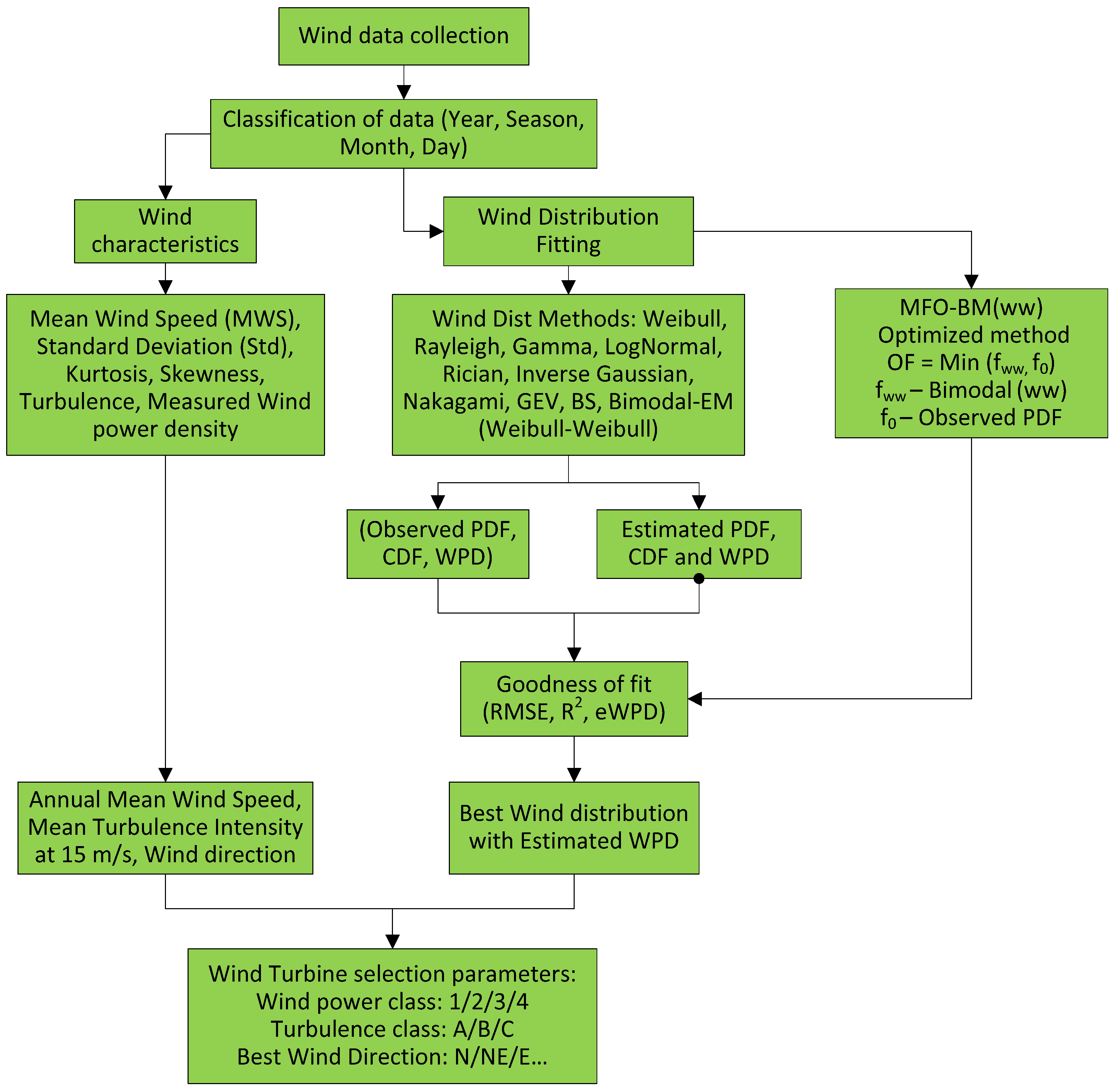
2. Wind Data Analysis Methods

Wind speeds in specific locations are subject to variation by the time of day, seasonal, and weather events due to the uneven heating of the earth’s surface. As well, the wind resource is varying (increase or decrease or made turbulent) by factors such as hilly area, bodies of water, buildings, and vegetative lands. The wind data analysis of different landscapes such as onshore, nearshore, and offshore is carried out in the subsequent sections. Later, wind characteristics, wind distribution fitting, and wind power densities are presented for the selected locations.

2.1. Wind Characteristics Parameters

Ground-level wind parameters are measured by meteorological instruments mounted on tall towers and other modern instruments like LiDAR and SODAR (Sonic detection and ranging) [27]. They act as a primary-data collection sensors for most wind resource assessment. The key parameters for any wind monitoring program are wind speed, wind direction, and air temperature. The parameters normally measured in a wind location are as follows:

• Average, standard deviation, minimum and maximum wind speed (m/s) are measured for wind generation suitability assessment, and turbine selection.
• Average, standard deviation and maximum gust direction (degrees) are estimated for optimizing wind turbines and understand the spatial distribution of wind
• Temperature (°C) and vertical wind speed (m/s) are used for the air density and turbulence application respectively to measure the average and minimum/maximum value.
• Average, standard deviation and minimum/maximum value of barometric pressure (kPa) are measured for air density applications
• Relative humidity (%) and solar radiation (W/m²) (average, minimum/maximum value) are measured for the icing and atmospheric analysis respectively.

2.2. Wind Speed Distribution Methods

The wind speed and its frequency of occurrence to form a wind distribution pattern is a critical piece of information. They are used to evaluate the power output of the wind turbine directly. The frequency of wind distribution denotes the number of intervals during period of data collected when the perceived wind speed falls within specific bins. They are normally occurred about 0.5 or 1 m/s space. They cover a minimum range of speeds described for the turbine power curve, i.e., 0 to 25 m/s and even more. The usual reports are presented in the bar chart/histogram and input as a table for software analysis. The probability density function is a mathematical one that visualizes the probable pattern of wind speed, which is random by nature in a continuous period. The detailed wind distribution models for the calculation of probability density function and cumulative distribution function [14] are presented in Appendix B.

2.3. Goodness of Fit

The goodness of fit is a statistical analysis method for qualifying the ten wind probability distributions considered for evaluation to match with actual data measured. The best scored root mean square error (RMSE) and correlation coefficient (R²) [11] finds the best fit wind distribution method for the defined location. They are used to determine the fitness of ten distributions. These can be calculated as follows:

2.3.1. Root Mean Square Value (RMSE)

RMSE estimate the residuals of the frequency of examined PDF (Probability density function) and the measured data.

$$RMSE={\left[\frac{1}{n}{\displaystyle \sum }_{i=1}^n{\left(y_i-x_i\right)}^2\right]}^{0.5}$$

(1)

where $y_i$ is the observed data plotted in a histogram, n stands for the number of bins and $x_i$ is an estimated PDF of wind distribution considered for evaluation. The evaluated RMSE value should be close to zero to form a best fit.

2.3.2. The Coefficient of Determination (R²)

The R² evaluates the linear correlation between predicted values from PDF functions and measured data.

$$R^2=1-\frac{{{\displaystyle \sum }}_{i=1}^n{\left(y_i-x_i\right)}^2}{{{\displaystyle \sum }}_{i=1}^n{\left(y_i-\overline{y}\right)}^2}$$

(2)

where $\overline{y}$ defines the mean of the total observed value and the value of R² lies between 0 to 1 (closer to 1 is the best fit).

3. Wind Site and Measurement Details

The wind data collected from two Indian states namely Gujarat and Tamilnadu are considered for analysis. These two states are pioneers in wind energy generation contributing to the Indian power grid in a higher stake. The wind data segregated into three categories such as onshore from Kayathar (Tamilnadu, India), offshore from Gulf of Khambhat (Gujarat, India), and nearshore from Jafrabad (Gujarat, India). The statistics of each location are presented in

Table 1. Measurement sensor data from wind stations.

Location	Landmass Meas. Sensor	Latitude and Longitude	Dataset Period	Interval	Recovery Rate
Kayathar (Tamilnadu)	Onshore (Mast)	8°56′42.50″ N, 77°43′24.12″ E	2014, 2015, 2016 (3 years)	10 min	100%
Gulf of Khambhat (Gujarat)	Offshore (LiDAR)	20°45′19.10″ N, 71°41′10.93″ E	12/2018 to 11/2019 (1 year)	10 min	75.85%
Jafrabad (Gujarat)	Nearshore (Mast)	20°53′29.81″ N, 71°27′35.68″ E	12/2018 to 11/2019 (1 year)	10 min	99.89%

.

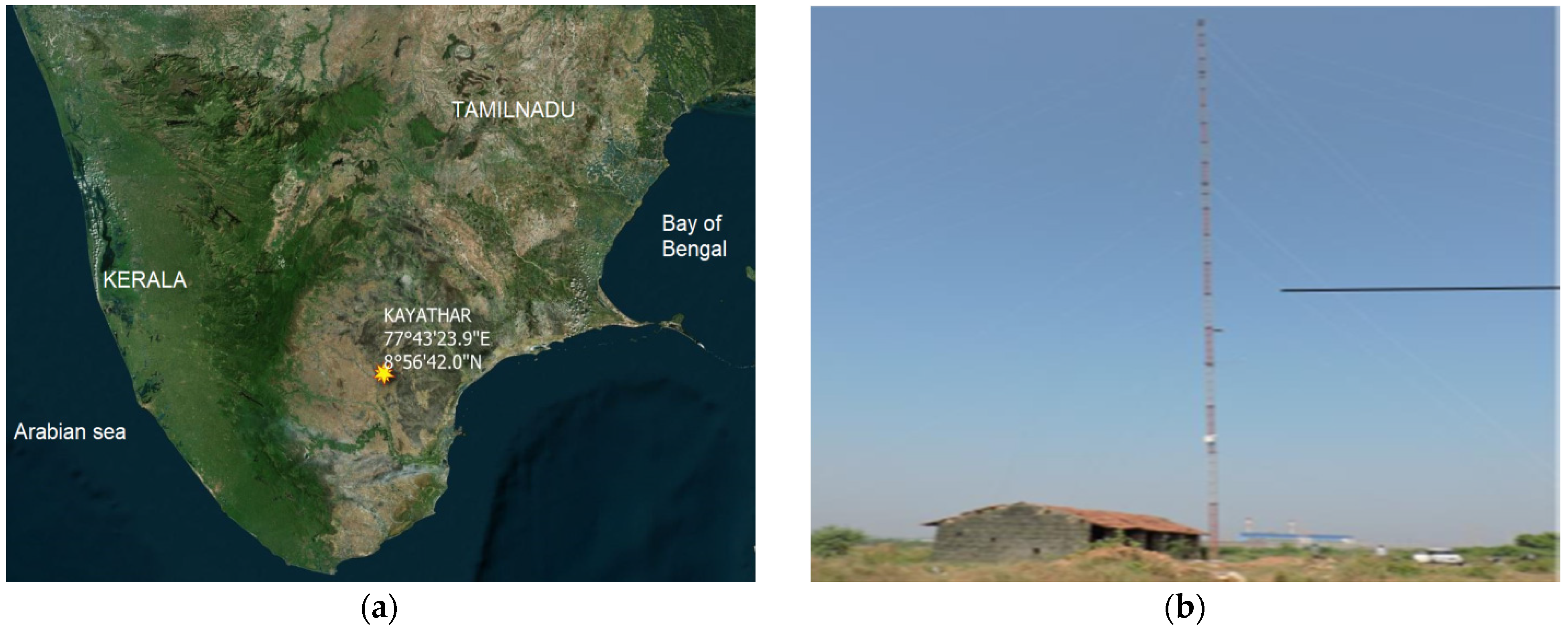
3.1. Kayathar (Tamilnadu)—Onshore Location

The Tamilnadu State, situated at the southeastern end of the Indian peninsula, comprises of a higher rate of humidity and temperature throughout the year. The annual rainfall received from the South–West monsoon (June to September) and the North–East monsoon (October to December) is 911.6 mm and temperature ranges between 20 °C and 38 °C in the plains [28]. Kayathar is a small town located in the southern part of the Tamilnadu. The mapping coordinates of Kayathar are 08°57′ N 77°48′ E and it is situated at 78 m elevation (altitude) above sea level. The geolocation of the targeted site is shown in Figure 1a. The wind data collected from the mast installed at a height of 120 m by the National Institute of Wind Energy (NIWE) (the central agency for wind energy developments in India). Wind data measured at Kayathar were recorded with an average of 10 min along with different altitudes, directions of wind flow, temperature, and pressure for three years between the years 2014 and 2016. This region experiences a template of monsoon variations from South–West and North–East monsoons. Therefore, the summer season is very hot with high humidity, and hence this site is prone to high windy during monsoons. The wind data collected from this site is classified into three categories likely seasonal, yearly, and monthly to evaluate the wind characteristics [29].

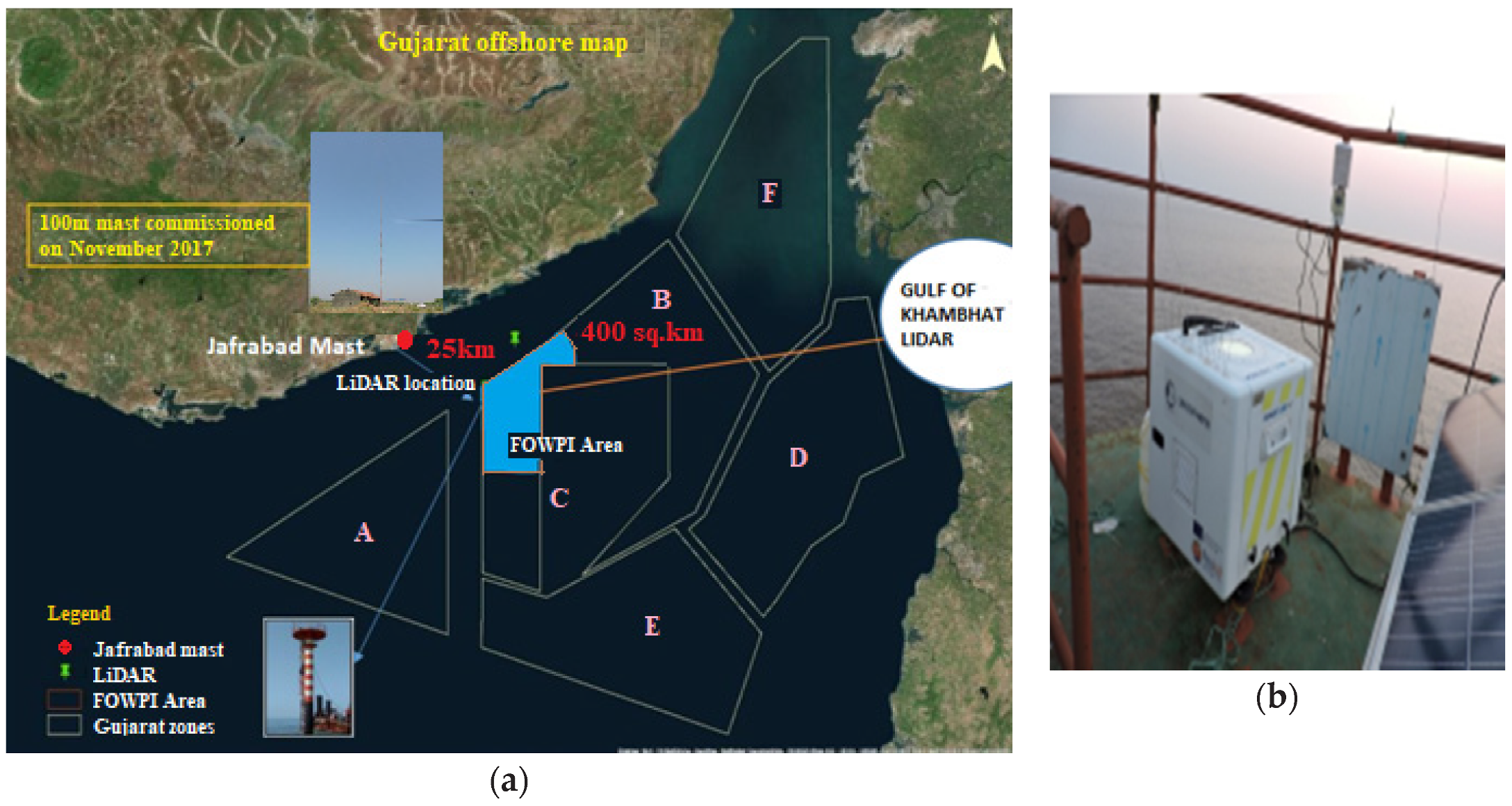
3.2. Gulf of Khambhat (Gujarat)—Offshore Location

Gujarat state has an international boundary with common border at the North–Western (NW) fringe [30]. It has a long coastline of about 1600 km, which is the longest among all states of the country with a geographical area of 1.96 lakh sq. km. It is situated between 20°1′ and 24°7′ North latitudes and 68°4′ and 74°4′ East longitudes with an elevation of about 9 m [30]. India earmarked the states Gujarat and Tamilnadu for pacing up rapidly towards offshore wind energy development through the supervision of the nodal ministry MNRE—Ministry of New and Renewable Energy and nodal agency NIWE—National Institute of Wind Energy). The offshore development activities are started with preliminary site assessments in Gujarat coastal area. The proposed location of the offshore wind farm is about 23 to 40 km off the coast from the Pipavav port, Gulf of Khambhat, Gujarat. It covers about 400 km² and the wind measurements and other data collections are through LiDAR.

Figure 2 displays the placement of the LiDAR instruments, showing a monopole structure erected in the Gulf of Khambhat at 20°45′19.10″ N, 71°41′10.93″ E with 25 km distance from the coast and 15 m water depth. The nearest port is Pipavav located at approximately 23 km from the Gujarat coast in the South–East direction. The monopole structure with a platform comprises of an anemometer, wind vane, temperature monitor, and pressure instruments are also commissioned. The LiDAR instrument is a wind cube configured for 12 various heights with a minimum height of 40 m and maximum height of 200 m. The overall data collected from LiDAR for the period from December 2018 to November 2019 is about 75.85% of the total, and the remaining 24% of data are not successful due to technical issues.

3.3. Jafrabad (Gujarat) Nearshore Location

The meteorological mast tower is installed with 100 m height at the Jafrabad coast in line of sight with the LiDAR location, at the distance of 25 km (Figure 1b). The main purpose of this installation is to correlate and validate with the LiDAR measurement for assessing offshore Gulf of Khambhat wind potential. The wind speed is measured from anemometers and temperature sensors placed at various levels such as 100, 80, 50, and 20 m above ground level. The wind direction sensors are positioned at 98, 78, and 48 m. This mast is installed at 20 53′29.81″ N, 71 27′35.68″ E with an altitude of 9 m above the ground level, with a mast height of 100 m. The wind data was collected with a 99.89% recovery rate for the period from December 2018 to November 2019.

3.4. Seasonal Wind Periods

The highest wind power potential in India concentrated on two major states, namely Tamilnadu [28] and Gujarat [29]. Concerning the classification of seasons for Gujarat and Tamilnadu states, the influence of seasonal winds from North–East monsoon (NEM) and South–West monsoon (SWM) are taken into consideration for analysis [30]. These seasons are grouped based on seasonal months, as follows:

Winter: January and February (2 months)

Summer: March, April, and May (3 months)

SWM: June, July, August, and September (4 months)

NEM: October, November, and December (3 months)

3.5. Moth Flame Optimization (MFO) Method

The application of artificial intelligence and soft computing techniques along with optimization is adopted in various activities. In this work, this method is implemented for estimating the parameters of the bimodal Weibull–Weibull method. The MFO algorithm [31] is a naturally inspired algorithm where moths are fancy insects, which are highly similar to the family of butterflies. The main inspiration of MFO is the navigation method of moths in nature, called transverse orientation. Moths navigate at night by maintaining a fixed angle to the moon. This is an effective mechanism for traveling long distances in a straight line [32]. It is considered as one of the promising metaheuristic algorithms and successfully applied in various optimization problems in a wide range of fields, such as power and energy systems, economic dispatch, engineering design, image processing, and medical applications. The working principle of MFO is based on the individuals/set of moths (M) called population and flame (F) is said to be the best solution for each moth. The moth-flame combination contains one flame per moth, which is considered to be as its best position. During the iteration, this flame will get updated if any better solution found. The matrix OM stores the corresponding fitness (objective) value, which can be written as follows:

$$M=\left[\begin{array}{cccc}{m}_{11}& m_{12}& \cdots & m_{1d}\\ m_{21}& m_{22}& \cdots & m_{2d}\\ ⋮& ⋮& ⋮& ⋮\\ m_{n1}& m_{n2}& \cdots & m_{nd}\end{array}\right]\mathrm{and}OM=\left[\begin{array}{c}I\left(m_{11},m_{12},\cdots ,m_{1d}\right)\\ I\left(m_{21},m_{22},\cdots ,m_{2d}\right)\\ ⋮\\ I\left(m_{n1},m_{n2},\cdots ,m_{nd}\right)\end{array}\right]=\left[\begin{array}{c}O{M}_1\\ O{M}_2\\ ⋮\\ O{M}_n\end{array}\right]$$

(3)

where n is the number of moths, I is the objective function, and d is the number of variables. Notably, each moth flies around its corresponding flame. Therefore, the flames matrix is the same size as the moths matrix [30]. The set of flames can be represented in the matrix F, while the matrix OF indicates the corresponding fitness value and can be written as follows.

$$F=\left[\begin{array}{cccc}{F}_{11}& F_{12}& \cdots & F_{1d}\\ F_{21}& F_{22}& \cdots & F_{2d}\\ ⋮& ⋮& ⋮& ⋮\\ F_{n1}& F_{n2}& \cdots & F_{nd}\end{array}\right]\mathrm{and}OF=\left[\begin{array}{c}I\left(F_{11},F_{12},\cdots ,F_{1d}\right)\\ I\left(F_{21},F_{22},\cdots ,F_{2d}\right)\\ ⋮\\ I\left(F_{n1},F_{n2},\cdots ,F_{nd}\right)\end{array}\right]=\left[\begin{array}{c}O{F}_1\\ O{F}_2\\ ⋮\\ O{F}_n\end{array}\right]$$

(4)

The main difference between moths and flames is the way they are treated and updated in each iteration. The moths are search agents moving around the search space, while flames are the best position of moths obtained by the current iteration [30]. The equation to find the best optimal value is given as:

$$Mi=S\left(M_i, F_j\right)$$

(5)

where M_i indicates the i-th moth, Fj indicates the j-th flame, and S is the spiral function. The spiral function of the moth is given as:

$$S\left(M_i,F_j\right)=D_i\cdot e^{bt}\cdot \cos \left(2\pi t\right)+F_j$$

(6)

where $D_i$ indicates the distance of the i-th moth for the j-th flame, b is a constant for defining the shape of the logarithmic spiral, and t is a random number. $D_i$ is calculated as follows:

$$S{D}_i=\left|F_i-M_i\right|$$

(7)

where F_i indicates the i-th flame. The moth can converge or exploit in the given search space by changing the value ‘t’ when the position of a moth gets changed. A mechanism to solve the number of flames during each iteration is mathematically defined as follows:

$$\mathrm{flame}no=\mathrm{round}\left(N-l\ast \frac{N-1}{\mathrm{T}}\right)$$

(8)

where N is the maximum number of flames, l is the number of current iteration and T is the maximum number of iterations. The objective function to be considered for minimization of estimated Bimodal Weibull distribution parameters by MFO and observed actual wind speed distribution is derived as:

$${\xi }^2={\displaystyle \sum }{\left(fest-fo\right)}^2$$

(9)

where $fest$ is the estimated value from bimodal-MFO and $fo$ is the observed data from the histogram:

$$fest=w1 \left(\frac{k1}{c1}\right){\left(\frac{v}{c1}\right)}^{k1-1}\exp \left(-{\left(\frac{v}{c1}\right)}^{k1}\right)+w2 \left(\frac{k2}{c2}\right){\left(\frac{v}{c2}\right)}^{k2-1}\exp \left(-{\left(\frac{v}{c2}\right)}^{k2}\right)$$

(10)

where, the parameters k1 and k2 are shapes, c1 and c2 stand for scales, w1 and w2 define weights and v terms the wind speed. The MFO pseudocode algorithm with program logic is derived in Appendix A and the flow chart for the MFO algorithm is described in Figure 3.

4. Results and Discussions

This segment outlines the statistical investigation of the wind data measured in the three different landscapes. A total of ten wind distribution functions are adopted to estimate the correctness of the distribution that best fits the wind speeds of the targeted location. Later, the optimization method, i.e., the MFO method is applied for parameter estimation and compared with ten wind distribution parameters. The MATLAB R2018b software with in-house developed code is used for estimating the parameters of ten wind distribution functions along with the MLM. Then, it is compared with the estimated parameters through MFO method using bimodal (Weibull–Weibull) distribution. As stated earlier, the goodness of fit is to evaluate the best wind distribution method with a lower rate of RMSE value nearer to zero. Additionally, the higher rate of R² should be nearer to one with reduced error fitting for evaluating the wind power density. Further, the results are grouped for the best wind power density with the selected distribution. Later, the annual mean wind speed along with mean turbulence intensity (15 m/s) are considered for categorizing the turbulence class for the turbine selection to form a standalone wind turbine/wind farm. The complete steps/procedures for the assessment of wind resources are given in Figure 4.

4.1. Wind Characteristics

The detailed wind statistical analysis for the Kayathar station (onshore), Jafrabad station (Mast-nearshore), and Gulf of Khambhat station (offshore) are presented in this section. The key characteristics of any wind assessment are to ascertain the wind resource feasibility such as mean wind speed, standard deviations of wind, turbulence intensity, and wind directions. The collected statistical analysis is used to determine the site eligibility for wind turbines, selection and energy yield to make the wind project technically viable. The statistical analysis of wind speed, wind direction, and its relation is represented by the wind rose plot. The mean wind speed over the periods for seasonal, monthly, and annual analysis represent the energy contained in the wind, and for the analysis of turbulence intensity to classify turbines. The PDF for fitting the wind speed distribution, wind power potential analysis, and statistical characteristics are presented in the following sections.

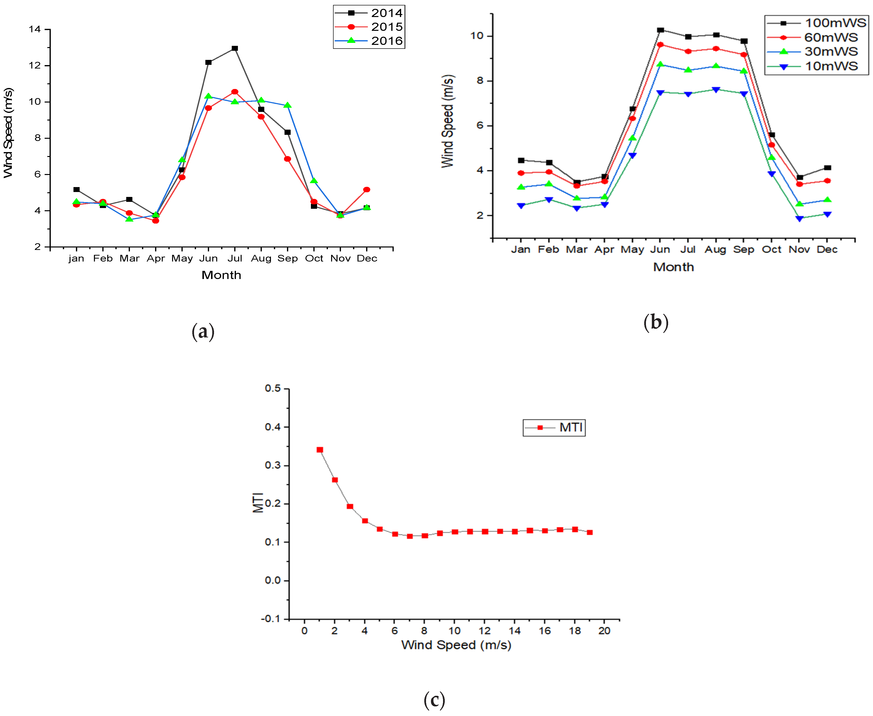
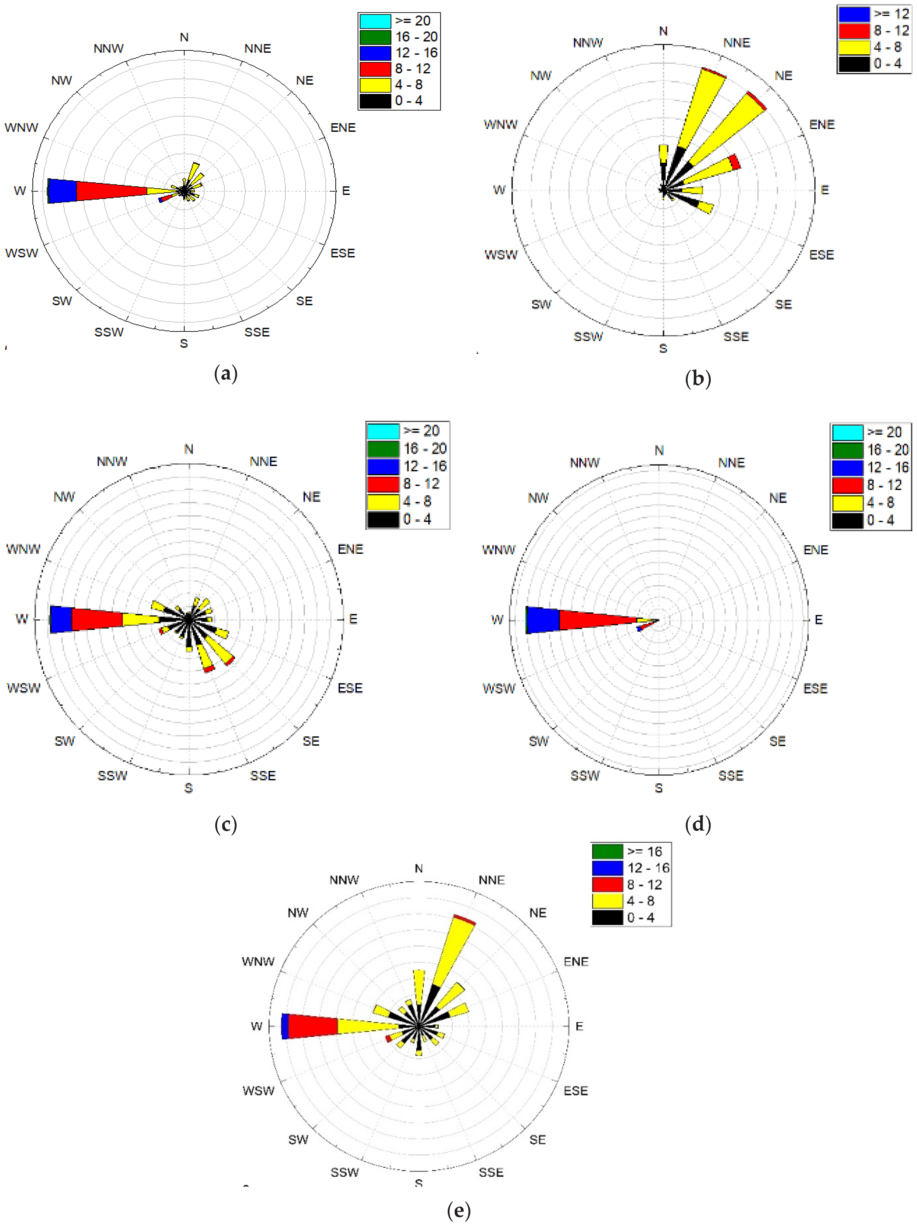
4.1.1. Kayathar Station (Onshore)

The annual mean wind speed (MWS), standard deviation, maximum wind speed, skew, and kurtosis in the Kayathar region between the years 2014 and 2016 are presented in

Table 2. Annual wind speed (100 m) statistics.

Year	Vmean (m/s)	Vrmc (m/s)	Vstd (m/s)	Vmax (m/s)	Vmin (m/s)	Vskew (m/s)	Vkurt	Vmedian	MTI (m/s)
2014	6.62	8.84	4.14	20.92	0.28	0.80	−0.31	5.34	0.17
2015	5.98	7.81	3.56	19.27	0.41	0.77	−0.32	4.96	0.18
2016	6.38	8.16	3.65	18.84	0.19	0.55	−0.70	5.51	0.17

and Figure 5a. The highest mean wind speed of about 6.62 m/s is recorded in the year 2014 with a maximum wind speed of 20.92 m/s for the same year. Further, the skewness factors of the wind speed are observed as a maximum of 0.8086 m/s in the year 2014 and a minimum of 0.5589 m/s in the year 2015. This skewness rate indicates the positive wind distribution with a moderate skew range between 0.5 to 1 [32]. The annual average kurtosis is recorded as −0.3190 and −0.7038 in the year 2014 and 2016 respectively. It specifies the shorter wind distribution and thinner tails than the normal distribution. The wind speed at various altitudes are measured and shown in Figure 5b. It is observed for different ranges such as 10, 30, 60, and 100 mWS. Additionally, the shear analysis power-law coefficient is evaluated and observed as 0.170.

Table 3. Kayathar wind characteristics—month wise.

Season	Vmean (m/s)	Vstd (m/s)	Vmax (m/s)	VSkew	VKurt	MTI (m/s)
Winter	4.43	1.69	10.36	0.50	−0.01	0.25
Summer	4.68	2.65	14.30	0.57	−0.39	0.16
SWM	10.03	2.74	18.52	−0.13	0.006	0.13
NEM	4.50	2.21	13.83	0.67	0.34	0.19
Annual	6.38	3.65	18.84	0.55	−0.70	0.17
January	4.48	1.49	9.66	0.45	−0.06	0.18
February	4.38	1.88	11.07	0.56	0.03	0.33
March	3.51	1.72	13.3	0.68	0.41	0.17
April	3.76	2.23	11.18	0.74	−0.46	0.17
May	6.78	3.99	18.44	0.27	−1.12	0.14
June	10.29	2.67	19.63	−0.09	0.18	0.13
July	9.98	3.53	19.81	−0.29	0.0004	0.14
August	10.07	2.48	17.05	−0.05	−0.15	0.13
September	9.79	2.29	17.6	−0.10	−0.009	0.13
October	5.62	3.01	16.54	0.60	−0.37	0.18
November	3.73	1.93	12.85	0.83	0.98	0.22
December	4.15	1.68	12.1	0.57	0.41	0.18

illustrates the seasonal wind speed peaks on the South–West monsoon period (SWM) of about 10.03 m/s and maximum seasonal wind speed observed as 18.52 m/s. Comparing the monsoon periods, the North–East monsoon (NEM) fetches a low wind mean speed of 4.5 m/s. The monthly mean wind speed is observed as having a maximum during June of 10.29 m/s and the maximum wind speed during July is 19.81 m/s. The monthly standard deviation is stable from January to March with an average value of 1.8 m/s. Further, it is observed as 3.99, 3.5, and 3.01 m/s for May, July, and October respectively during the peaks in monsoon periods due to seasonal winds. The mean turbulence intensity (MTI) is estimated as a ratio between the standard deviation of the experiential wind speed every 10 min and the mean observed wind speed for the same period. Additionally, the turbulence is higher at a low wind speed as shown in Figure 5c. The defined location, namely the Kayathar wind station, falls on turbulence category ‘B’ (as per International Electrotechnical Commission (IEC) standard) with MTI at 15 m/s of 0.132, i.e., 13.2% (Table 3).

Figure 5 shows the annual wind statistics at 100 m height, wind speed at different altitude and intensity of turbulence. It is observed that the wind speed increases on higher altitudes. When considering the 10 m, the wind speed attained a scale of 2 m/s and further reaches about 4 m/s (100 m). It is known fact that the wind power is the cubic of wind speed; it is suggested to erect the turbines at higher altitude and hub height to obtain higher wind energy extraction. The wind speed observed in the year 2016 was not great, and particularly relatively lower than 2015 and 2014 due to climatic changes. Table 3 shows the observed wind speed of the Kayathar station for seasonal case and it recorded better characteristics. It is situated in the southern part of Tamilnadu and produces more wind power during the SWM, which stakes the major portion of state demand.

Furthermore, the annual maximum wind speeds hinge on wind direction; the West direction observed a maximum wind speed of 10.26 m/s (38.66%) followed by WSW and WNW, i.e., 11.27% and 7.57% respectively, as shown in

Table 4. Kayathar wind directions—annual occurrence.

Direction Sector	Direction Name	Mean (m/s)	Max (m/s)	Std. Dev. (m/s)	Wind Occ. (%)
348.75°–11.25°	N	3.14	13.46	1.25	1.73
11.25°–33.75°	NNE	4.25	15.05	1.68	6.50
33.75°–56.25°	NE	4.76	20.63	1.82	6.51
56.25°–78.75°	ENE	4.82	14.03	2.03	4.67
78.75°–101.25°	E	4.62	13.38	2.24	2.84
101.25°–123.75°	ESE	3.73	16.54	1.68	4.16
123.75°–146.25°	SE	4.20	11.82	1.98	3.51
146.25°–168.75°	SSE	4.82	11.18	2.29	3.58
168.75°–191.25°	S	3.48	11.77	1.85	2.37
191.25°–213.75°	SSW	2.75	12.12	1.39	1.60
213.75°–236.25°	SW	2.97	10.11	1.53	1.86
236.25°–258.75°	WSW	5.44	19.87	3.50	11.27
258.75°–281.25°	W	10.26	22.86	3.30	38.66
281.25°–303.75°	WNW	6.06	18.82	3.00	7.57
303.75°–326.25°	NW	3.11	13.48	1.35	1.88
326.25°–348.75°	NNW	3.07	11.94	1.30	1.21

. The second maximum wind generation of NEM in NE wind direction is observed as 6.51%, with a mean wind speed of 4.766 m/s followed by NNE (North–Northern east) of 6.50%. The wind rose plots exposed in Figure 6 indicate the influence of South–West and North–East monsoons. The North–East monsoon influenced the wind direction during October to December, and the West direction shifts to N–NNE (Northern NNE). During SWM periods, (i.e., June–September) wind directions are found to be West and WSW (West southern west). It also represents the main wind direction from the West and ranges between 258.75°–281.25° during the South–West. The winter season experiences NEM winds and influences at the end of the South–West monsoon period. The summer wind rose plot experiences wind from SWM and the wind direction from SE–SSE (Southeast–South Southeast) and Western direction. It indicates that the Kayathar region experiences maximum wind power from the Southwest direction. During low-wind periods from NEM and winter seasons, the wind speed reduced relatively which deteriorate to low wind generation.

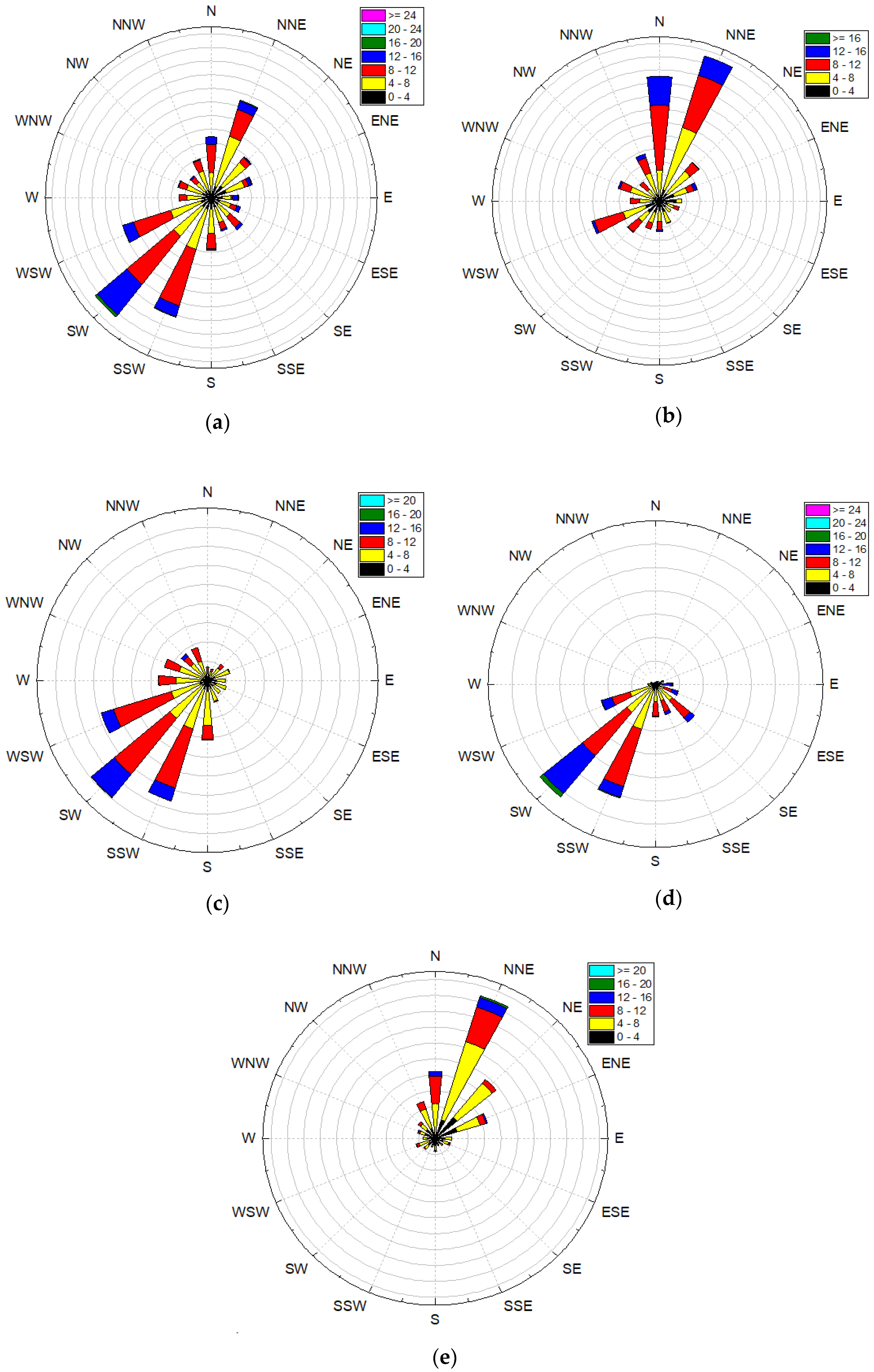
4.1.2. Gulf of Khambhat (Gujarat Offshore) Station

The mean wind speed (MWS) collected from LiDAR measurements at various heights (40 to 200 m) are presented in Figure 7 for the period of December 2018 to November 2019. It is observed that the wind speed attained an increased rate for higher altitudes with higher hub height (100 to 160 m) which fetches more wind power. The wind speed of the Gulf of Khambhat during prevailing months is high compared with the Kayathar region, particularly during winter and NEM periods, which are suitable for sustained wind generation.

Table 5. Annual and seasonal parameter of Gulf of Khambhat.

Param	Winter	Summer	SWM	NEM	Annual
Vmean(m/s)	7.12	7.56	9.04	5.74	7.51
Vstd(m/s)	3.31	3.07	3.44	3.01	3.44
Vmax(m/s)	15.28	16.87	20.26	17.02	20.26
MTI(m/s)	0.06	0.07	0.07	0.10	0.08
VSkew	0.15	0.08	0.05	0.72	0.25
VKurt	−0.83	−0.70	−0.52	0.22	0.57

shows the monthly-maximum mean wind speed in July (10.13 m/s) and low mean wind speed in November (4.81 m/s). Considering the 100 m measurements for analysis, the annual mean wind speed and maximum wind speed during June are observed as 7.59 and 22.99 m/s respectively. The shear analysis power-law coefficient is perceived as 0.0782 based on the measured wind speeds at various altitudes. In comparison with the Kayathar onshore shear coefficient, the Gulf of Khambhat is less due to its offshore landscape by nature. The wind rose plot for seasonal periods is plotted and presented in Figure 8. The major wind directions during SW (Southwest) monsoon are observed in the SW–South direction and during the NE (Northeastern) monsoon on the North–NE direction. The annual and seasonal wind rose plots are shown in Figure 8. The maximum range of annual wind speed occurred in SSW and SW direction. Regarding seasonal changes, the winter season took the maximum wind that occurs in the North to NE direction.

Table 6. Gulf of Khambhat monthly wind parameters.

Month	Vmean (m/s)	Vrmc (m/s)	Vstd (m/s)	Vmax (m/s)	Vmin (m/s)	Vskew	Vkurt
January	7.61	9.06	3.64	15.34	0.43	0.02	−1.06
February	6.52	7.64	2.91	15.89	0.3	0.11	−0.65
March	6.62	7.62	2.71	15.93	0.4	0.30	−0.37
April	7.25	8.36	3.04	16.42	0.35	0.08	−0.65
May	9.01	9.97	3.18	17.27	0.49	−0.40	−0.43
June	9.51	10.63	3.46	22.99	0.37	−0.007	−0.43
July	10.13	11.18	3.54	18.74	0.54	−0.57	−0.26
August	8.86	10.07	3.38	20.39	1.1	0.50	−0.04
September	7.56	8.47	2.79	15.25	0.5	−0.06	−0.66
October	5.40	6.84	2.90	17.98	0.42	1.07	1.35
November	4.81	5.97	2.51	19.39	0.43	0.60	0.70
December	6.65	8.02	3.22	17.37	0.2	0.43	−0.55

displays the maximum seasonal wind speed parameters of about 20.26 m/s and maximum mean wind speed of 9.04 m/s during the June to September (SWM) season. The standard deviation is stable throughout the year in all the seasons with an average value of 3.2 m/s. The minimum mean wind speed during NEM periods (October–December) is recorded as 5.74 m/s. Additionally, the annual wind speed of 7.511 m/s and maximum wind speed of 20.263 m/s is observed. The NEM period of the Gulf of Khambhat recorded the low wind speed of 5.74 m/s and the remaining periods show the average range of about 7 m/s, i.e., winter and summer.

The month-based wind speed shown peak on July (10.13 m/s) and maximum wind speed occurred during June (22.99 m/s) due to SEM. The low wind speed occurred during October and November, i.e., 5.4 and 4.8 m/s respectively, due to NEM. The skewness factor of the wind speed obtained a maximum value of 1.07 during October. The annual skewness is recorded as 0.25. It indicates that the wind distribution is positive with a moderate skew, and its range falls between 0.5 to 1. The annual kurtosis rate (0.57) indicates that the wind distribution is shorter; tails are thinner than the normal distribution.

The annual wind direction obtained a maximum value at the SW (Southwest) direction of about 15.8% with a mean wind speed of 9.8501 m/s. Further, SSW (South Southwest) and WSW (West Southwest) obtained about 15.8% and 8.7% respectively, due to SWM as shown in

Table 7. Wind direction annual statistics of the Gulf of Khambhat.

Sector	Direction Name	Mean (m/s)	Median (m/s)	Min (m/s)	Max (m/s)	Std. Dev. (m/s)	Wind Occ. (%)
348.75°–11.25°	N	7.83	7.75	0.37	15.05	3.12	10.17
11.25°–33.75°	NNE	7.09	6.73	0.4	17.98	3.13	11.07
33.75°–56.25°	NE	5.73	5.09	0.42	18.12	3.02	5.82
56.25°–78.75°	ENE	5.47	4.53	0.47	20.21	3.43	3.72
78.75°–101.25°	E	6.48	4.79	0.41	22.99	4.51	2.92
101.25°–123.75°	ESE	6.65	5.49	0.44	20.27	3.89	2.93
123.75°–146.25°	SE	7.27	7.3	0.41	16.95	3.42	4.07
146.25°–168.75°	SSE	6.35	5.66	0.43	15.74	3.29	3.53
168.75°–191.25°	S	6.76	6.7	0.47	14.05	2.85	4.66
191.25°–213.75°	SSW	8.44	8.73	0.3	18.17	2.89	13.05
213.75°–236.25°	SW	9.80	10.06	0.48	20.39	3.48	15.80
236.25°–258.75°	WSW	8.13	8.44	0.49	18.74	3.22	8.75
258.75°–281.25°	W	6.22	5.93	0.35	14.06	2.89	3.24
281.25°–303.75°	WNW	5.69	5.55	0.68	11.82	2.56	2.86
303.75°–326.25°	NW	5.96	5.7	0.41	16.42	3.18	3.08
326.25°–348.75°	NNW	6.50	6.63	0.61	13.84	2.90	4.25

. The next maximum wind direction occurred in the NNE (North Northeast) of about 11.07%, with a mean wind speed of 7.0987 m/s followed by North direction (10.17%) with a mean wind speed of 7.83%. The wind direction starts at N–NNE–NE during the winter season initially, and moves towards the South–Southwest direction during summer with the traces of the SWM season picking up. Later, the peaks have risen during the SWM with SW–S direction and finally through the NEM season in the N–NE direction. The major wind directions are obtained in the S–SW and N–NE direction during the seasonal periods. The turbulence intensity for offshore LiDAR data is plotted in Figure 7b, and its mean value took place at 15 m/s (5.9%). As per the IEC standard, it falls on the turbulence Ç category. On comparison with the onshore Kayathar station, the MTI value is low due to the offshore area. From the above discussed wind characteristics, the Gulf of Khambhat shows better results, with specifically steady wind speed and low turbulence intensity. These positive factors provide sustained wind generation and help the wind farm planners to invest in offshore wind power production in the region of Gulf of Khambhat.

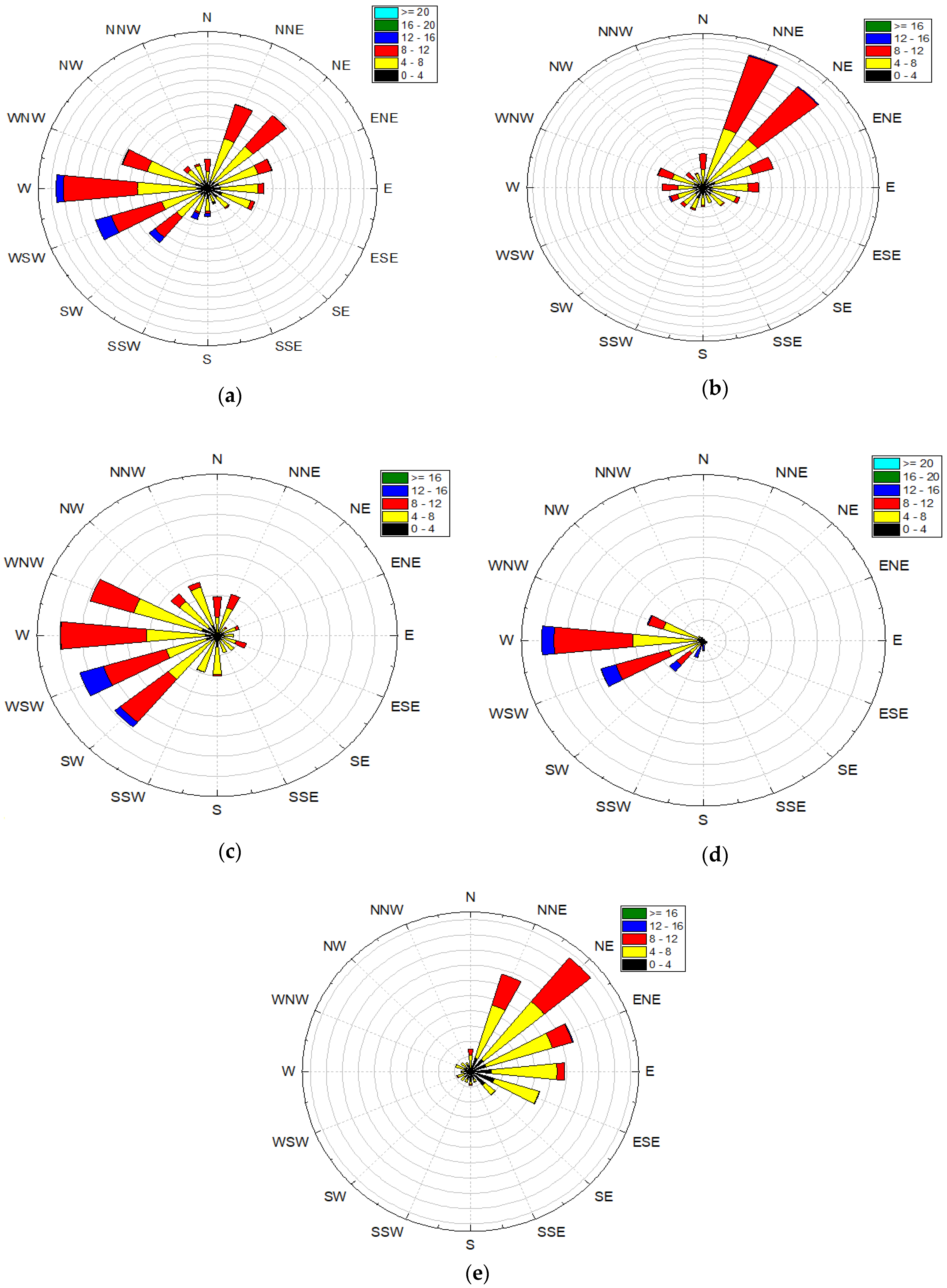
4.1.3. Jafrabad (Gujarat—Nearshore)

The wind data collected from mast anemometers with various altitudes (20–100 m) for the period of December 2018 to November 2019 is considered. The mean wind speed (MWS) data collected from mast measurements at various heights (10 to 100 m) for the same period is presented in Figure 9. The maximum mean wind speed is attained about 8.92 m/s at 100 m in June and a low mean wind speed of 5.11 m/s in November is perceived. Further, the comparison of mean wind speed gain is made while increasing the altitudes (June) at 20 and 100 m are 6.48 m/s, and 8.92 m/s, respectively. Wherein, the 100 m measurements are taken for analysis and the annual mean wind speed of 6.99 m/s at 100 m is observed. The shear analysis power-law coefficient is observed as 0.0228 based on the measured wind speeds at various altitudes. On comparison with the Kayathar onshore shear coefficient, the Jafrabad nearshore is less due to its coastal area. The distance between the Jafrabad wind station and Gulf of Khambhat (offshore) is 25 km. The wind speed behaves dynamically with different altitudes, and some steady wind speed patterns are observed at 100 and 80 m. The wind turbine with the hub height of 80 m shows steady wind generation, and is suitable for efficient power production.

The annual wind direction from the wind rose plots are shown in Figure 10. The maximum wind direction occurs in SW to West direction. Regarding the winter season and NEM, the wind direction goes toward the NNE to East direction. During the SWM season and summer monsoon periods, the majority of wind occurs in the SW to WNW direction.

Table 8. Seasonal parameter—Jafrabad.

Wparm	Winter	Summer	SWM	NEM	Annual
Vmean (m/s)	6.67	7.08	8.01	5.74	6.99
Vstd (m/s)	2.58	2.63	2.97	2.43	2.83
Vmax (m/s)	13.38	14.75	17.47	13.72	17.47
Skew	−0.008	0.09	0.27	0.30	0.29
Kurtosis	0.85	−0.42	0.36	0.47	0.26

and

Table 9. Monthly wind profile—Jafrabad.

Month	Vmean (m/s)	Vrmc (m/s)	Vstd (m/s)	Vmax (m/s)	Vmin (m/s)	Vskew	Vkurt
January	6.84	7.76	2.68	14.49	0.42	−0.04	−0.85
February	6.48	7.38	2.58	13.70	0.37	0.03	−0.74
March	6.49	7.24	2.31	13.13	0.52	0.10	−0.47
April	6.70	7.60	2.62	15.0	0.31	−0.02	−0.42
May	8.02	8.93	2.88	15.56	0.51	−0.14	−0.47
June	8.92	10.11	3.41	19.09	0.36	0.28	−0.62
July	8.56	9.41	2.90	17.34	0.53	−0.43	−0.38
August	8.07	8.88	2.61	17.79	1.80	0.55	0.30
September	6.45	7.37	2.54	14.05	0.47	0.46	−0.14
October	5.53	6.38	2.28	13.78	0.28	0.41	−0.002
November	5.11	6.01	2.28	19.36	0.24	0.31	−0.06
December	6.57	7.50	2.63	13.17	0.54	0.07	−0.87
Annual	6.99	8.02	2.83	17.47	0.54	0.29	−0.26

display the annual, seasonal, and monthly wind parameters.

Table 10. Directional statistics—Jafrabad.

Sector	Direction Name	Mean (m/s)	Std. Dev. (m/s)	Wind Occ. (%)
348.75°–11.25°	N	7.40	2.36	3.19
11.25°–33.75°	NNE	7.21	2.23	9.42
33.75°–56.25°	NE	7.35	2.41	10.15
56.25°–78.75°	ENE	6.23	2.38	6.69
78.75°–101.25°	E	5.39	2.02	5.59
101.25°–123.75°	ESE	5.04	1.96	4.89
123.75°–146.25°	SE	4.45	1.93	2.81
146.25°–168.75°	SSE	4.97	3.27	1.74
168.75°–191.25°	S	6.05	3.85	3.03
191.25°–213.75°	SSW	6.71	3.96	3.47
213.75°–236.25°	SW	7.81	3.07	7.50
236.25°–258.75°	WSW	8.61	3.12	11.63
258.75°–281.25°	W	7.99	2.57	15.04
281.25°–303.75°	WNW	6.65	2.41	8.89
303.75°–326.25°	NW	5.45	2.26	3.11
326.25°–348.75°	NNW	5.14	1.86	2.77

shows the annual wind direction at the SW direction with maximum stake of 15.04% and mean wind speed of 7.991 m/s. Later, the WSW and WNW shares about 11.631% and 8.891% respectively, due to the South–West monsoon. The next maximum wind direction of 10.158% occurred in the NE with a mean wind speed of 7.335 m/s, followed by an NNE direction (9.42%) with a mean wind speed of 7.217%.

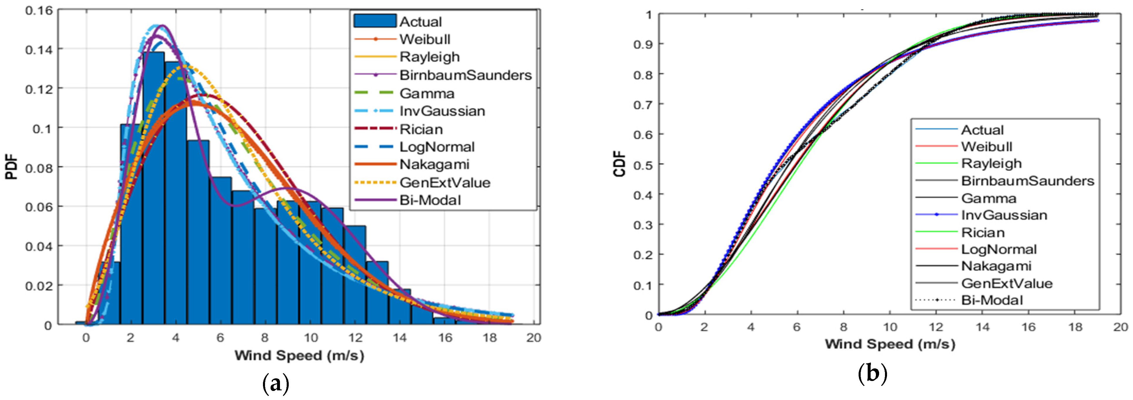
4.2. Wind Distribution Fitting

For estimating the wind energy potential, accurate wind distribution modeling is essential to extract wind power meritoriously. The performance of targeted location wind potential assessment hinges on the selection of the PDF to illustrate the computed wind speed behavior plotted in the frequency distribution.

The collected wind speed data to fit into ten numbers of wind distribution such as Weibull, Rayleigh, Birnbaum–Sandras (BS), gamma (GM), inverse Gaussian (IG), Rician (RI), lognormal (LN), Nakagami (NK), GEV and bimodal Weibull–Weibull (BM) distribution methods. The bimodal WW method is adopted, since the visual traces of probability distribution function have similarity in the bimodal with two peaks. The bimodal nature is predicted by numerical calculations of mean and standard deviation [33,34]. The goodness of fit and best-fitted wind distribution is ascertained with RMSE and R² methods by comparing actual measured data with individual wind distribution methods through PDFs. In this work, three methods are adopted, namely the maximum likelihood method (MLM), expectation-maximization algorithm (EM) and moth flame optimization (MFO). The bimodal-Weibull–Weibull methods are used to estimate the parameters of wind speed distributions. The EM method consists of two steps, namely the expectation-step (E-step) and the maximization-step (M-step). The E-step computes the conditional expectation and the M-step maximizes the expectation. The parameters of the bimodal and multimodal distribution are estimated by an iterative procedure until convergence is reached. Additionally, the bimodal WW parameters (Appendix B) were estimated through the MFO with objective function by minimizing the error between estimated and observed PDF. The distribution of wind speed data (also known as wind frequency distribution) is presented by histogram plots which are a usual method of presenting wind data for a specific year. The histogram displays the percentage of time of occurrence of each wind speed ranges.

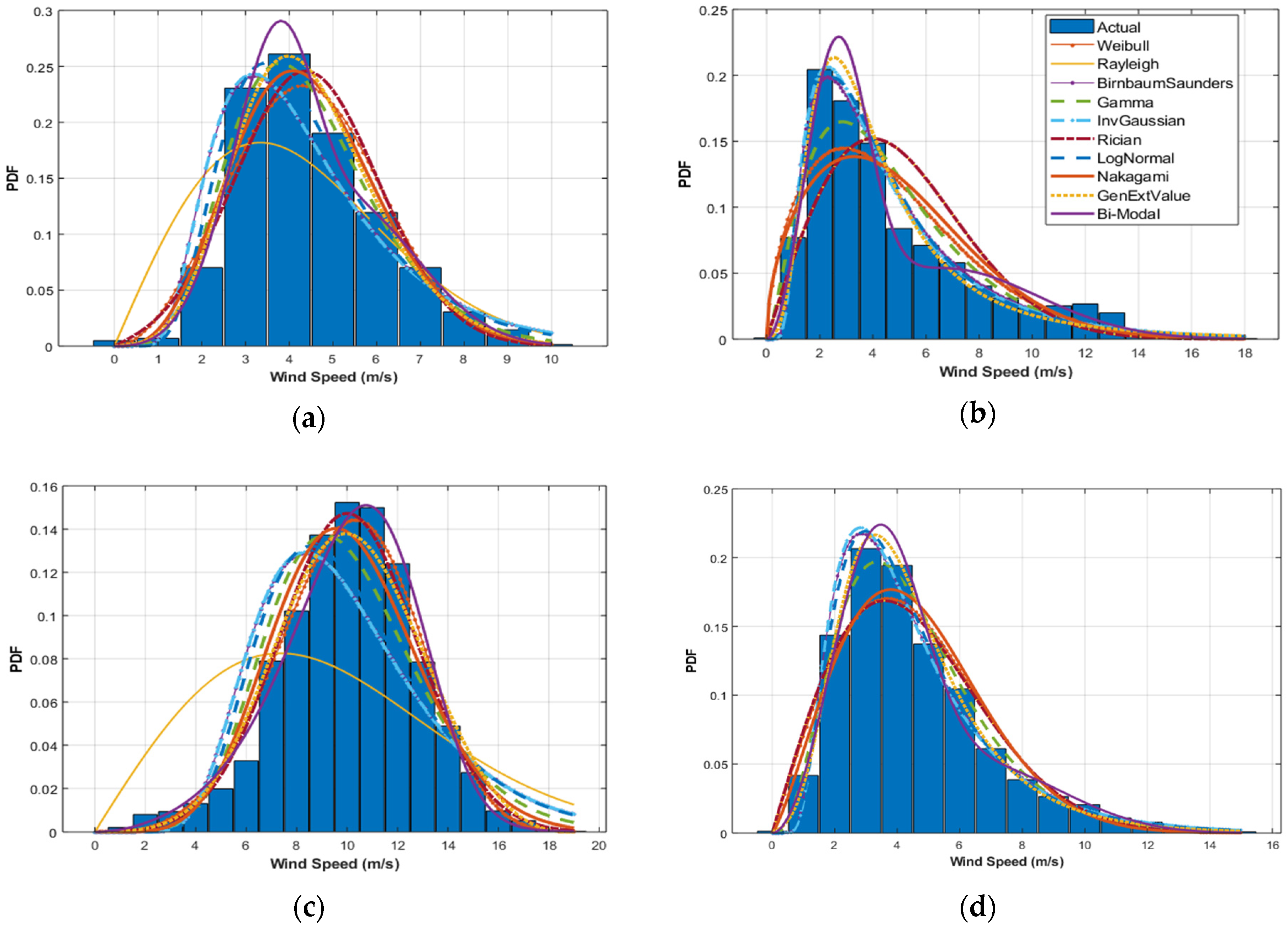
4.2.1. Kayathar Station (Onshore)

The annual wind speed observed at the 100 m hub height with estimated parameters using 10 distributions through probability distribution function (PDF) and cumulative probability distribution (CDF) plots are shown in Figure 11. The observed wind speed plotted into frequency distribution is fitting with other distributions to observe the difference in the fitting of each distribution with real histogram data.

The wind distribution from the bimodal Weibull–Weibull method closely follows the peaks of observed histogram wind patterns. The other distribution plots seem to be under fitting and close fit to the observed histogram as per the pictorial observation. Figure 12 shows the seasonal wind speed pattern by estimated parameters with distribution functions and plotted with PDF functions. The visual examination of PDF—specifically the Rayleigh distribution—behaves distinctly from other distributions during winter, summer, and SEM monsoon periods. During winter, Rayleigh performs well owing to the incidence of low wind speed.

It is also observed that the Rayleigh distribution suffers from histogram fitting during the winter and Southwest Monsoon periods. The bimodal behavior observed during the summer season and the curve follows the histogram variations.

4.2.2. Bi-Modal Behavior

The bi-modal WW method was applied to observe the data in two parts with different weightage, as shown in

Table 11. Kayathar bimodal estimated parameters.

Seasons	Vmean (m/s)	mu1	mu2	sigma1	sigma2	w1	w2	k1bm	c1bm	k2bm	c2bm	bmc1	bmc2
Annual	6.38	3.36	8.96	1.27	2.98	0.45	0.54	2.87	3.76	3.29	9.99	1.43	3.05
Winter	4.43	3.51	5.06	0.84	1.68	0.40	0.59	4.69	3.84	3.29	5.64	0.64	−0.15
Summer	4.69	2.74	7.28	1.05	3.08	0.57	0.42	2.82	3.08	2.54	8.21	1.25	2.43
SWM	10.03	8.54	10.4	3.27	2.32	0.22	0.77	2.82	9.59	5.13	11.39	0.35	−2.70
NEM	4.51	3.45	6.71	1.29	2.51	0.67	0.32	2.89	3.87	2.90	7.52	0.90	0.66

. It is estimated using bimodal methods through the EM (expectation-maximization) algorithm and the values are plotted on each part along with weightage, mean speed, standard deviation, shape, and scale parameters. The bmc1 and bmc2 are the bimodality numerical check apart from visual analysis. Where bmc1 = |μ2 − μ1|/(2 (σ1 × σ2) ^(1/2)) when bmc1 > 1. Likewise, bmc2 == |μ2 − μ1|/(2* min (σ1, σ2)) when bmc2 > 2. (μ1 and μ2 are means, and σ1 and σ2 are standard deviations of 2 parts of the bimodal model.

The wind distribution examination in the Kayathar region falls on multiple peaks and differs from normal bell-shaped histogram curves. The bimodal behavior is exclusively analyzed with the bimodal Weibull–Weibull method. Figure 13 shows the bimodal behavior of the annual and winter season. The annual season has more bimodality than winter through visual analysis, as given in Table 11, i.e., bmc1 and bmc2 estimation. Wherein, winter comprises a lesser range of bmc1 and bmc2 of 0.64 and −0.1511 respectively with the annual value of 1.43 and 3.05 for bmc1 and bmc2 respectively.

Table 12. Kayathar wind distribution estimated parameters.

Dist	Parameter	Annual	Winter	Summer	SWM	NEM
	Vmean (m/s)	6.38	4.43	4.69	10.04	4.51
WB	k—shape	7.21	4.96	5.28	11.03	5.11
	c—scale	1.84	2.93	1.61	4.19	2.05
	Mean	6.41	4.42	4.73	10.02	4.53
	Std	3.61	1.63	2.99	2.70	2.32
RY	$\sigma$—scale	5.20	3.33	3.99	7.35	3.60
	Mean	6.52	4.17	5.00	9.21	4.51
	Std	3.40	2.18	2.61	4.82	2.36
NK	$\mu$—shape	0.88	2.00	0.75	3.24	1.13
	$\omega$—scale	54.17	22.22	31.85	108.07	25.88
	Mean	6.43	4.43	4.82	10.00	4.57
	Std	3.57	1.60	2.92	2.83	2.24
IG	$\mu$—mean	6.38	4.43	4.69	10.04	4.51
	$\mathsf{\lambda }$—shape	12.27	19.58	9.02	80.13	13.79
	Mean	6.38	4.43	4.69	10.04	4.51
	Std	4.60	2.11	3.38	3.55	2.58
RI	b—location	0.68	4.06	0.23	9.63	0.27
	a—scale	5.18	1.69	3.99	2.76	3.59
	Mean	6.52	4.43	5.00	10.04	4.51
	Std	3.41	1.59	2.61	2.70	2.36
BS	$\beta$—scale	5.16	3.99	3.81	9.46	3.91
	$\gamma$—shape	0.68	0.46	0.68	0.35	0.55
	Mean	6.37	4.42	4.70	10.03	4.51
	Std	4.43	2.08	3.27	3.54	2.54
GM	θ—scale	2.82	6.94	2.54	11.00	3.91
	k—shape	2.26	0.63	1.85	0.91	1.15
	Mean	6.38	4.43	4.70	10.04	4.51
	Std	3.80	1.68	2.95	3.03	2.28
GEV	$\mu$—location	0.05	-0.13	0.31	-0.28	0.07
	$\sigma$—scale	2.81	1.43	1.80	2.79	1.70
	$\xi$—shape	4.58	3.77	3.01	9.07	3.40
	Mean	6.38	4.43	4.84	10.06	4.51
	Std	3.92	1.59	4.59	2.78	2.42
LN	µ—mean	1.66	1.41	1.34	2.26	1.37
	$\mathsf{\sigma }$—scale	0.64	0.41	0.65	0.33	0.53
	Mean	6.53	4.49	4.72	10.13	4.55
	Std	0.64	0.41	0.65	0.33	0.53

shows the yearly and seasonal parameters from the observed wind speed by ten wind distribution models with the parameter estimation from the maximum likelihood method. The MATLAB developed in-house software program codes are used for parameter estimation.

Table 13. Kayathar wind distribution PDF fitness.

Distribution Metrics
Season	Fitness	Annual	Winter	Summer	SWM	NEM
Vmean		6.39	4.43	4.70	10.04	4.51
BM	RMSE	0.00	0.01	0.01	0.01	0.01
	R2	0.99	0.99	0.96	0.98	0.99
WB	RMSE	0.02	0.02	0.02	0.01	0.02
	R2	0.82	0.93	0.87	0.99	0.94
RY	RMSE	0.02	0.05	0.03	0.04	0.02
	R2	0.76	0.76	0.73	0.46	0.94
NK	RMSE	0.02	0.02	0.03	0.01	0.02
	R2	0.81	0.97	0.82	0.95	0.95
IG	RMSE	0.02	0.03	0.01	0.03	0.01
	R2	0.91	0.90	0.98	0.78	0.97
RI	RMSE	0.02	0.03	0.03	0.01	0.02
	R2	0.76	0.92	0.73	0.99	0.94
BS	RMSE	0.01	0.03	0.01	0.03	0.01
	R2	0.91	0.90	0.98	0.78	0.98
GM	RMSE	0.02	0.01	0.02	0.02	0.01
	R2	0.86	0.99	0.91	0.91	0.99
GEV	RMSE	0.02	0.01	0.01	0.01	0.00
	R2	0.81	0.98	0.98	0.98	1.00
LN	RMSE	0.02	0.02	0.01	0.02	0.01
	R2	0.90	0.97	0.98	0.83	0.99
Good Fit	RMSE	BM	Gamma	IG	Rician	GEV
Good Fit	R2	BM	Gamma	IG	Rician	GEV

displays the goodness of fit methods of RMSE and R² between estimated wind distribution parameters and observed parameters by the ten distributions PDF. The annual wind distribution rate of the Kayathar region shows lower RMSE and R² value of 0.004 and 0.9878 respectively. The seasonal wind distribution fitness such as winter (best fit by gamma method), summer (inverse gamma), SWM (Rician method) and winter season (GEV method) are observed. From the Kayathar wind distribution fitting observations, the bimodal Weibull–Weibull wind distribution is best suited, compared to other wind speed distributions on annual wind flow analyses.

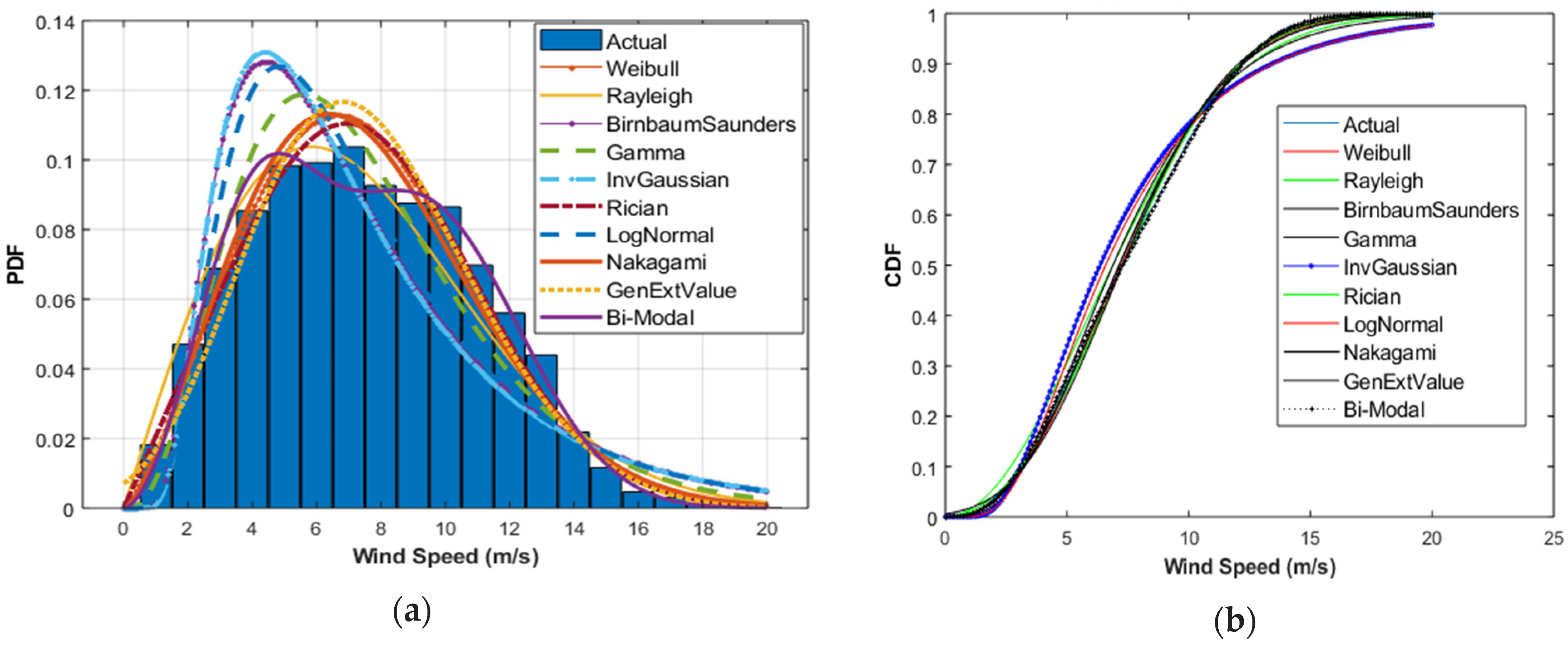
4.2.3. Gulf of Khambat (Offshore) Wind Distribution

The annual wind speed observed at 100 m with estimated parameters by 10 distributions through probability distribution function (PDF) and cumulative probability distribution (CDF) plots in the Gulf of Khambhat region is presented in Figure 14.

The Gulf of Khambhat wind distribution presented in a frequency distribution histogram plot is shown in the above Figure. Some bimodal traces and the bimodal distribution follows the peaks of a histogram, and most of the wind distributions seem to be slightly over fit. As per the observations, all the wind distributions follow the histogram if there are no bimodal traces. On bimodal traces, all distributions are slightly deviating except bimodal wind distributions.

Figure 15 shows the seasonal wind speed pattern by the estimated parameters using distribution functions and plotted with PDF functions. The Rician, Weibull and Nakagami seem to follow the histogram. Whereas, the bimodal distribution seems to be a close fit. The Rayleigh distribution shown in the orange line in the PDF plot during the Southwest monsoon deviates from the observed frequency histogram plot. The Rayleigh distribution looks to be fit on low wind speed seasons only.

Table 14. Gulf of Khambhat bimodal estimated parameters.

Season	mu1	mu2	sigma1	sigma2	w1	w2	k1bm	c1bm	k2bm	c2bm	bmc1	bmc2
Ann	4.18	9.01	1.66	2.95	0.31	0.69	2.72	4.70	3.36	10.04	1.09	1.51
Win	3.35	8.32	1.31	2.82	0.24	0.76	2.78	3.76	3.24	9.29	1.30	2.36
Sum	4.63	9.29	1.66	2.32	0.37	0.63	3.05	5.18	4.51	10.18	1.19	1.34
SWM	5.68	10.62	2.04	2.78	0.32	0.68	3.04	6.36	4.29	11.67	1.04	0.86
NEM	3.78	7.59	1.57	2.87	0.48	0.52	2.60	4.26	2.87	8.51	0.90	0.67

shows the bi-modal WW method parameters. The bmc1 and bmc2 are the bimodality numerical check apart from visual analysis.

The wind distribution analysis in the Gulf of Khambhat region falls on multiple peaks. Figure 15 shows the bimodal behavior of the annual and winter season. The annual season has less bimodality than winter through visual analysis. The estimated value of bmc1 and bmc2 are observed as 1.29 and 2.35 respectively. The annual value has a lower score of bmc1 and bmc2 of about 1.09 and 1.50 respectively.

Table 15. Gulf of Khambhat wind distribution estimated parameters.

Dist	Param	Annual	Winter	Summer	SWM	NEM
Vmean		7.51	7.13	7.56	9.05	5.75
WB	k—shape	8.48	8.05	8.51	10.15	6.50
	c—scale	2.33	2.30	2.68	2.87	2.02
	Mean	7.52	7.13	7.56	9.05	5.76
	Std	3.43	3.28	3.05	3.42	2.98
RY	$\sigma$—scale	5.84	5.56	5.77	6.85	4.59
	Mean	7.32	6.97	7.23	8.58	5.75
	Std	3.83	3.64	3.78	4.48	3.01
NK	$\mu$—shape	1.24	1.20	1.53	1.72	1.05
	$\omega$—scale	68.31	61.77	66.64	93.71	42.10
	Mean	7.49	7.10	7.53	9.01	5.78
	Std	3.49	3.37	3.15	3.54	2.95
IG	$\mu$—mean	7.51	7.13	7.56	9.05	5.75
	$\lambda$—shape	20.02	17.96	26.08	35.49	13.92
	Mean	7.51	7.13	7.56	9.05	5.75
	Std	4.60	4.49	4.07	4.57	3.69
RI	b—location	5.96	5.60	6.61	8.13	0.65
	a—scale	4.05	3.90	3.39	3.71	4.57
	Mean	7.51	7.13	7.56	9.04	5.75
	Std	3.45	3.31	3.09	3.45	3.01
BS	$\beta$—scale	6.39	6.01	6.64	8.06	4.82
	$\gamma$—shape	0.59	0.60	0.52	0.49	0.61
	Mean	7.49	7.11	7.55	9.03	5.73
	Std	4.49	4.37	4.01	4.51	3.60
GM	θ—scale	3.96	3.77	4.96	5.63	3.42
	k—shape	1.90	1.89	1.52	1.61	1.68
	Mean	7.51	7.13	7.56	9.05	5.75
	Std	3.78	3.67	3.40	3.81	3.11
GEV	$\mu$—location	−0.19	−0.25	−0.26	−0.25	−0.02
	$\sigma$—scale	3.21	3.19	3.01	3.38	2.43
	$\xi$—shape	6.15	5.91	6.44	7.77	4.37
	Mean	7.49	7.10	7.55	9.04	5.73
	Std	3.41	3.24	3.04	3.44	3.05
LN	µ—mean	1.88	1.83	1.92	2.11	1.60
	$\sigma$—scale	0.56	0.57	0.50	0.47	0.59
	Mean	7.70	7.32	7.71	9.20	5.86

shows the yearly and seasonal parameters from the observed wind speed by ten wind distribution models with the parameter estimation from the maximum likelihood method.

Table 16. The goodness of fit values for the Gulf of Khambhat.

Season	Fitness	Annual	Winter	Summer	SWM	NEM
BM	RMSE	0.00	0.01	0.01	0.01	0.01
	R2	0.99	0.95	0.98	0.98	0.97
WB	RMSE	0.01	0.01	0.01	0.01	0.01
	R2	0.97	0.93	0.95	0.96	0.99
RY	RMSE	0.01	0.01	0.02	0.02	0.01
	R2	0.96	0.91	0.84	0.79	0.99
NK	RMSE	0.01	0.01	0.01	0.01	0.01
	R2	0.97	0.92	0.93	0.94	0.98
IG	RMSE	0.02	0.03	0.02	0.02	0.02
	R2	0.78	0.68	0.73	0.73	0.90
RI	RMSE	0.01	0.01	0.01	0.01	0.01
	R2	0.98	0.94	0.94	0.96	0.99
BS	RMSE	0.02	0.03	0.02	0.02	0.02
	R2	0.79	0.70	0.75	0.74	0.91
Gamma	RMSE	0.01	0.02	0.02	0.01	0.01
	R2	0.92	0.85	0.87	0.89	0.99
GEV	RMSE	0.01	0.01	0.01	0.01	0.01
	R2	0.96	0.90	0.94	0.96	0.97
LN	RMSE	0.02	0.02	0.02	0.02	0.01
	R2	0.83	0.74	0.78	0.79	0.93
Good Fit	RMSE	BM	WB	BM	BM	Rayleigh
	R2	BM	BM	BM	BM	Rayleigh

shows the goodness of fit methods of RMSE and R² between estimated wind distribution parameters and observed parameters by ten distribution models. The annual wind distribution pattern follows the bimodal-WW wind distribution model with a lower rate of RMSE and R² values.

By comparing the annual best fit, the bimodal WW distribution performed well compared with the other distributions as indicated with the R² and RMSE values of 0.98 and 0.004, respectively. During seasonal periods, the bimodal WW performed well on summer and SWM periods. The Weibull and BM share the best fit during the winter season, and the Rayleigh distribution performed well during the North East monsoon (NEM) period.

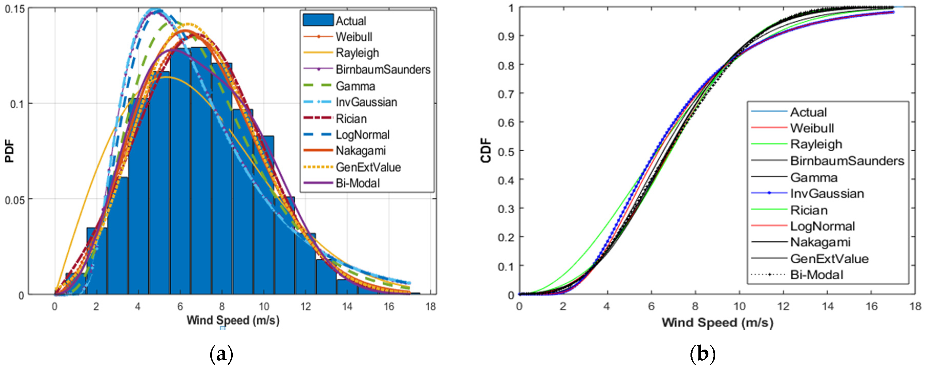
4.2.4. Jafrabad Station (Nearshore) Distribution Fitting

Figure 16 shows the annual wind speed observed at the 100 m hub height with computed parameters by 10 distributions of PDF and CDF plots in the Jafrabad nearshore region. The wind distribution representation of the Jafrabad plot such as inverse Gaussian, gamma, and lognormal distribution looks to over fit the histogram. Whereas, the Weibull, Rician, Nakagami and bimodal distributions appear to fit the frequency distribution plot. The seasonal wind speed pattern of the estimated parameters by the distribution functions and plotted with PDF is shown in Figure 17. The bimodality is observed in the winter season of the Jafrabad plot with peaks of histogram and summer season. The Rayleigh shows the usual trend, which has diverged during the Southwest monsoon. It behaves worse during the high-wind period of the SEM. The other wind distributions, such as the Rician, Weibull and Nakagami, are responding well during the high-wind periods.

Table 17. Jafrabad bimodal estimated parameters.

Season	mu1	mu2	sigma1	sigma2	w1	w2	k1bm	c1bm	k2bm	c2bm	bmc1	bmc2
Annual	4.47	7.96	1.58	2.61	0.28	0.72	3.10	5.01	3.36	8.88	0.86	0.33
Winter	4.68	8.81	1.61	1.52	0.51	0.48	3.20	5.23	6.75	9.44	1.32	1.09
Summer	3.71	7.57	1.24	2.42	0.12	0.87	3.30	4.15	3.46	8.43	1.12	1.38
SWM	5.77	9.58	1.83	2.60	0.41	0.58	3.50	6.42	4.12	10.55	0.87	0.16
NEM	3.85	7.10	1.40	2.09	0.41	0.58	3.01	4.32	3.78	7.87	0.95	0.45

shows the bi-modal WW method parameters. The bmc1 and bmc2 are the bimodality numerical check, apart from visual analysis. There is no bimodality in comparison with other locations, due to the lower value of bmc1 and bmc2 of about 0.860 and 0.328, respectively. Figure 17 shows the bimodal behavior of winter season with the bmc1 and bmc2 scores of 1.321 and 1.088, respectively, with not much visual changes on bimodality during the summer season.

Table 18. Jafrabad wind distribution estimated parameters.

Dist.	Param	Annual	Winter	Summer	SW-Mon	NE-Mon
	Vmean	6.99	6.67	7.08	8.02	5.75
WB	k—shape	7.87	7.50	7.94	8.99	6.48
	c—scale	2.66	2.84	2.94	2.93	2.54
	Mean	6.99	6.68	7.08	8.02	5.76
	Std	2.83	2.55	2.62	2.98	2.42
RY	$\sigma$—scale	5.34	5.06	5.34	6.05	4.42
	Mean	6.69	6.34	6.70	7.58	5.53
	Std	3.50	3.32	3.50	3.96	2.89
NK	$\mu$—shape	1.58	1.67	1.82	1.89	1.47
	$\omega$—scale	56.93	51.21	57.13	73.11	38.98
	Mean	6.98	6.65	7.06	8.01	5.74
	Std	2.87	2.65	2.70	3.00	2.45
IG	$\mu$—mean	6.99	6.67	7.08	8.02	5.75
	$\lambda$—shape	26.86	25.99	31.60	40.51	20.27
	Mean	6.99	6.67	7.08	8.02	5.75
	Std	3.57	3.38	3.35	3.57	3.06
RI	b—location	6.11	5.96	6.42	7.27	4.90
	a—scale	3.13	2.81	2.83	3.18	2.74
	Mean	6.99	6.67	7.08	8.01	5.74
	Std	2.85	2.59	2.64	2.98	2.45
BS	$\beta$—scale	6.22	5.94	6.39	7.32	5.07
	$\gamma$—shape	0.50	0.49	0.46	0.43	0.52
	Mean	6.98	6.66	7.07	8.01	5.74
	Std	3.52	3.34	3.32	3.54	3.02
GM	θ—scale	5.26	5.45	6.05	6.47	4.85
	k—shape	1.33	1.22	1.17	1.24	1.19
	Mean	6.99	6.67	7.08	8.02	5.75
	Std	3.05	2.86	2.88	3.15	2.61
GEV	$\mu$—location	−0.18	−0.31	−0.25	−0.19	−0.18
	$\sigma$—scale	2.65	2.59	2.58	2.79	2.25
	$\xi$—shape	5.86	5.79	6.11	6.85	4.78
	Mean	6.98	6.66	7.08	8.00	5.74
	Std	2.82	2.55	2.62	2.95	2.40
LN	µ—mean	1.85	1.80	1.87	2.00	1.64
	$\sigma$—scale	0.48	0.47	0.44	0.42	0.50
	Mean	7.10	6.78	7.18	8.09	5.84

shows the yearly and seasonal estimated parameters from the observed wind speed by ten distribution models with the parameter estimation from the maximum likelihood method.

It is observed that the bimodal WW performed well during the winter periods particularly on the SWM and NEM periods (

Table 19. Jafrabad goodness of fit estimated parameters.

Season	Fitness	Annual	Winter	Summer	SWM	NEM
		6.99	6.67	7.08	8.02	5.75
BM	RMSE	0.01	0.01	0.01	0.01	0.01
	R2	0.99	0.98	0.98	0.99	0.98
WB	RMSE	0.00	0.02	0.01	0.01	0.01
	R2	1.00	0.89	0.99	0.98	0.97
RY	RMSE	0.02	0.03	0.03	0.02	0.02
	R2	0.89	0.75	0.77	0.80	0.91
NK	RMSE	0.01	0.02	0.01	0.01	0.01
	R2	0.99	0.87	0.97	0.99	0.98
IG	RMSE	0.02	0.03	0.03	0.02	0.02
	R2	0.84	0.71	0.76	0.90	0.85
RI	RMSE	0.01	0.02	0.01	0.01	0.01
	R2	0.99	0.88	0.99	0.97	0.96
BS	RMSE	0.02	0.03	0.03	0.02	0.02
	R2	0.85	0.72	0.77	0.90	0.86
GM	RMSE	0.01	0.02	0.02	0.01	0.01
	R2	0.96	0.83	0.91	0.97	0.96
GEV	RMSE	0.01	0.02	0.01	0.01	0.01
	R2	0.99	0.89	0.99	0.98	0.97
LN	RMSE	0.02	0.03	0.02	0.01	0.02
	R2	0.88	0.75	0.81	0.92	0.89
Good Fit	RMSE	Weibull	BM	Weibull	BM	BM
	R2	Weibull	BM	Rician	BM	BM

). The value of R² (0.989) shared the best fit during summer, whereas the Weibull shares the best fit with RMSE (0.006). By summarizing all the locations, the bimodal WW stands at the top, and the Jafrabad Weibull distribution ranked as the best fit. The annual PDF parameters estimated from the ten distributions are compared with the proposed optimization method using the moth flame optimization algorithm are in the subsequent section.

4.3. Optimization Methods for Parameter Estimation

Optimization Parameters Comparison

The parameters estimated from the wind distribution methods in the previous sections through unimodal and EM algorithm for bimodal (BM-EM) are compared with annual bimodal Weibull parameters through the moth flame optimization method. The estimation of the moth flame method parameter is presented in

Table 20. BM–MFO wind distribution estimated parameters.

Method	Station	Mean	k1	c1	k2	c2	w1	w2
BM-EM	Kayathar	6.39	2.87	3.77	3.29	9.99	0.46	0.54
BM-MFO	Kayathar		2.63	3.82	3.01	9.89	0.46	0.54
BM-EM	GoK	7.51	2.72	4.70	3.36	10.04	0.31	0.69
BM-MFO	GoK		2.44	5.04	3.37	9.96	0.30	0.70
BM-EM	Jafrabad	6.99	3.10	5.01	3.36	8.88	0.28	0.72
BM-MFO	Jafrabad		2.95	5.08	2.99	8.41	0.16	0.84

. The optimization parameter is projected through the MFO with the objective function for the bimodal Weibull distribution.

The wind parameters from the MFO method, PDF fitness analysis with RMSE and R² method, and the snapshot of WPD results are presented in

Table 21. Optimization PDF fitness.

Method	Station	RMSE	R2	eWPD%	WPD
Pactual	Kayathar				334.17
BM-EM	Kayathar	0.005	0.99	0.08	333.89
BM-MFO	Kayathar	0.004	0.99	0.00	334.17
Pactual	GoK				431.53
BM-EM	GoK	0.005	0.99	0.22	430.56
BM-MFO	GoK	0.004	0.99	0.00	431.53
Pactual	Jafrabad				318.18
BM-EM	Jafrabad	0.005	0.99	0.45	316.76
BM-MFO	Jafrabad	0.003	1.00	0.68	318.18
WB-Unimodal	Jafrabad	0.003	1.00	0.68	316.03

. The MFO parameters are estimated in two stages by satisfying the PDF objective function firstly with minimum RMSE/R² value. Then, the over fit and under fit of wind power density calculated from estimated parameters from optimization is tuned with MFO optimization again for higher accuracy. The observed results satisfy both the lower RMSE/R² value and the annual wind power density. It is accurately estimated through the MFO method. The results of MFO for Kayathar, Jafrabad, and the Gulf of Khambhat (GoK) outperform the bimodal parameters estimated through the EM algorithm and MFO stands top-graded in all the stations.

4.4. Wind Power Density Analysis (WPD)

The WPD value is the major factor for the wind energy potential assessment of a targeted location. It also helps to evaluate the economic feasibility to form a potential wind farm. The modelling of WPD outlines the distributions of wind energy at several wind speed and it is proportional to the cube of wind speed. Its value is represented in W/m² and depends on the wind location, air density, and wind speed. It is derived as follows:

$$WPD=\frac{P}{A}=\frac{1}{2}\rho v^3$$

(11)

where P is the wind power measured in watts, A stands for a swept area in m², $\rho$ states the air density ($\rho$ = 1.225 kg/m³), and v represents the wind speed in m/s. Considering all these, the distribution of wind speed is taken into account and then WPD can be expressed as:

$$\frac{P}{A}=\frac{1}{2}\rho {{\displaystyle \int }}_0^{\infty }{v}^{3}f\left(v\right)dv$$

(12)

For evaluating the WPD of a particular distribution, the wind power density distribution function f(v) can be expressed as:

$$\frac{P}{A}=\frac{1}{2}\rho v^{3}f\left(v\right)$$

(13)

The best fit of WPD is calculated as follows:

$$eWPD=\left(\frac{\left(WPDo-WPDest\right)}{WPDo}\right)100\%$$

(14)

where $WPDo$, the observed wind power density, $WPDest$ is the estimated values from distribution fitting, and $eWPD$ is the error between observed and estimated values.

Comparison of Wind Power Density

The comparison of annual WPD with estimated MFO parameters and seasonable wind power density for the three locations are given in

Table 22. Annual WPD comparison with MFO and other methods.

WPD Annual Comparison		GoK Annual	Jafrabad Annual	WPD Annual Fitness Comparison
Dist.	Kayathar Annual			Distribution	Kayathar Annual	GoK Annual	Jafrabad Annual
Actual	334.17	431.53	318.18
BM-MFO	334.17	431.53	318.185	BM-MFO	5.42 × 10−8	5.81 × 10−10	−1.409 × 10−5
BM-EM	333.89	430.54	316.76	BM-EM	0.08	0.23	0.45
WB	325.23	430.55	316.03	WB	2.68	0.23	0.68
RY	319.76	445.6	330.17	RY	4.31	−3.26	−3.77
BS	319.05	447.39	324.34	BS	4.53	−3.67	−1.93
GM	323.06	448.22	323.65	GM	3.32	−3.87	−1.72
IG	312.96	443.16	322.83	IG	6.35	−2.69	−1.46
RI	320	431.11	315.26	RI	4.24	0.1	0.92
NK	325.25	434.01	317.14	NK	2.67	−0.58	0.33
GEV	310.55	423.73	314.85	GEV	7.07	1.81	1.05
LN	317.4	455.52	328.18	LN	5.02	−5.56	−3.14

and

Table 23. Wind power density.

Dist.	Kayathar Winter	Summer	SWM	NEM	GoK Winter	Summer	SWM	NEM	Jafrabad Winter	Summer	SWM	NEM
Actual	76.45	170.80	751.97	111.58	370.79	399.83	653.26	225.29	266.13	310.66	450.83	183.59
Bimodal EM(WW)	75.67	168.67	750.22	110.19	359.69	398.02	652.35	222.89	263.94	308.88	449.94	181.97
WB	75.54	156.24	748.65	106.16	341.26	395.26	649.57	219.07	255.79	307.45	447.10	180.98
RY	78.83	146.27	715.72	106.94	328.76	398.12	657.39	219.67	235.35	304.32	439.72	187.25
BS	78.20	161.23	762.86	112.67	283.22	379.98	637.78	225.76	222.95	296.18	428.90	182.70
GM	76.15	150.80	769.73	104.86	317.66	396.48	658.32	221.09	242.02	306.61	440.03	184.01
IG	78.00	161.12	761.83	113.11	278.06	376.72	633.71	223.84	221.01	294.55	427.05	181.56
RI	74.49	146.33	753.27	106.99	344.94	396.46	651.02	219.82	256.04	307.38	444.62	180.83
NK	75.00	155.61	757.78	104.41	335.75	395.91	652.69	218.08	250.37	306.87	443.05	181.33
GEV	74.77	153.03	766.27	106.14	349.27	392.36	650.64	214.73	259.20	307.47	443.06	178.76
LN	78.76	156.70	774.63	112.23	289.81	387.29	650.40	226.53	227.56	300.51	432.14	184.80

respectively.

The different landscapes of three locations such as offshore, nearshore, and onshore are considered for the analysis. Wind power density is evaluated after carrying goodness of fit with RMSE and R² using probability distribution methods. The goodness of fit indicates the wind power density and demonstrates the best distribution suits for the selected location.

Table 24. Wind power density (WPD) error metrics.

Kayathar					Gulf of Khambhat				Jafrabad
Season	Win	Sum	SWM	NEM	Win	Sum	SWM	NEM	Win	Sum	SWM	NEM
BM-EM	1.02	1.25	0.23	1.25	0.30	0.04	0.04	−0.29	0.82	0.57	0.20	0.89
WB	1.19	8.53	0.44	4.86	7.96	0.56	0.56	2.76	3.88	1.03	0.83	1.43
RY	−3.10	14.36	4.82	4.16	11.34	−0.63	−0.63	2.49	11.57	2.04	2.46	−1.99
BS	−2.30	5.60	−1.45	−0.97	23.62	2.37	2.37	−0.21	16.22	4.66	4.87	0.49
GM	0.39	11.71	−2.36	6.03	14.33	−0.77	−0.77	1.87	9.06	1.30	2.40	−0.23
IG	−2.00	5.67	−1.31	−1.37	25.01	2.99	2.99	0.64	16.95	5.18	5.27	1.10
RI	2.56	14.33	−0.17	4.12	6.97	0.34	0.34	2.43	3.79	1.05	1.38	1.50
NK	1.90	8.89	−0.77	6.43	9.45	0.09	0.09	3.20	5.92	1.22	1.73	1.23
GEV	2.20	10.40	−1.90	4.87	5.80	0.40	0.40	4.69	2.60	1.03	1.72	2.63
LN	−3.00	8.25	−3.01	−0.58	21.84	0.44	0.44	−0.55	14.49	3.27	4.15	−0.66
GF	BM	BM	BM	BM	BM	BM	BM	IG	BM	BM	BM	BS

represent the wind power density calculated from different distributions along with measured value during seasonal periods for three selected locations. Additionally, the annual WPD shares (region wise) of Jafrabad, Gulf Khambhat, and Kayathar are shown in Figure 18. The percentage shares of the SW monsoon take the upper hand in all three sites compared to other seasonal shares. Moreover, Figure 19 shows the monthly wind power density statistics using monthly WPD analysis for Kayathar station. The bimodal method scores better during February, April, July, August, and September (five months), whereas GEV distribution scores best during March, October, November, and December (four months) followed by Weibull during May and June as the best fit. For monthly wind power density of Gulf of Khambhat, BM scores better except February, June, and November whereas Rician distribution scores best during February and November followed by Weibull during June. For Jafrabad region monthly WPD analysis, BM scores better except for in April, May, and August, whereas the Rician distribution scores best during April. The generalized extreme value (GEV) distribution scored better during May, and the Weibull during August was the best fit.

Figure 19c represents the wind power density share in the different seasons by comparing each region. Gulf of Khambhat (offshore) shares about 37% of maximum wind power density during SWM and minimum during the NEM period with 15%. The winter and summer have a steady share of 22% and 26% respectively. The Gulf of Khambhat (GoK) has the advantage of steady wind power density, due to the advantage of offshore characteristics which is free from wind obstruction comparing with landmass. Jafrabad shows a similar pattern of WPD with peak WPD during the SWM of 40% and minimum on the North East period from October to December (about 14%). During winter and summer, WPD shares about 24% and 26% respectively. Kayathar displays wide marginal variations on WPD share with peaks during the SWM of about 68% and low WPD during North-East monsoon of 10% share. The winter stakes about 7% and summer share about 15% of the rest wind power density. Finally, the wind power class of Kayathar region falls on Class 2, Gulf of Khambhat falls on Class 3 and Jafrabad falls on Class 2 [35].

4.5. Research Findings

The wind energy potential assessments for selected locations of different landscape are evaluated using bimodal factors along with ten wind distribution methods and MFO optimization methods. The summary of the outcomes is represented in

Table 25. Research statistics in onshore, nearshore, and offshore.

S. No	Annual Parameter (@ 100 m)	Kayathar (Onshore)	Gulf of Khambhat (Offshore)	Jafrabad (Nearshore)
1	Mean wind speed (m/s)	6.38	7.51	6.99
2	Standard deviation (m/s)	3.65	3.44	2.83
3	Max. wind speed (m/s)	18.8	20.26	17.4
4	Skew	0.55	0.25	0.29
5	Kurt	−0.70	0.57	0.26
6	MTI at 15 (m/s)	13.2%	5.9%	6.4%
7	Shear power law index	0.17	0.07	0.02
8	Mean cubic wind speed	8.16	8.88	8.02
9	WPD (observed) W/m2	334.17	431.53	318.18
10	Turbulence category	B	C	C
	Wind power class	2	3	2
11	Wind distribution fit (Rank)	BM-MFO BM-EM Nakagami	BM-MFO Rician BM-EM and Weibull	BM-MFO Nakagami BM-EM
12	WPD (Estimated)	333.89	431.11	317.14
13	Best wind direction	W—38% WSW—11% WNW—7.57% NE—6.51% NNE—6.50%	SW—15.8% SSW—13.05% NNE—11.07% N–10.17% WSW—8.75%	W—15.04% WSW—11.63% NE—10.158% NNE—9.421% WNW-8.891%
14	Wind power density share	Winter—7% Summer—15% SWM—68% NEM—10%	Winter—22% Summer—24% SWM—40% NEM—14%	Winter—22% Summer—26% SWM—36% NEM—15%

.

The research findings on three different landmasses onshore, offshore and nearshore are presented. The offshore location attained a mean wind speed of 7.51 m/s, with wind power density of 431 m/s² and low turbulence intensity of 5.9%. It has the great advantage of exploring offshore wind energy extraction, by comparison with other onshore and nearshore wind stations. The proposed methodology (MFO–Bimodal Weibull–Weibull) performed well in all the three-wind location. The estimation of accurate wind distribution fit and wind power density are achieved using the moth flame optimization method (on estimating wind distribution parameters) in comparison with the maximum likelihood method. The selection of technologies for better wind resource assessment is the prime motive for ascertaining the accurate wind potential in targeted location. The commercially available wind analysis software should be tuned by incorporating the latest developments and observation of concepts from these types of research studies to cope the practical field conditions. This research study demonstrates the comparison of different wind distribution methods using different parameter estimation methods. It can be used to select the best wind distribution method from available methodologies. Though the proposed method shows numerous advantages over other methods, limitations such as number of iterations, number of moths, and measured quality of wind speed data are considered before adopting this method. Moreover, the measured data from field instruments are properly calibrated for high accuracy in results. The data collection during wind resource assessment and data loggers from instruments should be closely monitored for ensuring the continuance of data.

In nutshell, this research explored the multiple wind distributions and their behavior on different landscapes using bimodality influences. In India, Tamil Nadu and Gujarat stand at the top on wind energy generation. During data collection for this research, certain issues are observed in day to practice on wind energy management. The major hurdle is the low voltage ride through (LVRT) issue [36]. Because the power generating plants must continue to operate through short periods of low grid voltage, and should not get disconnected from the grid. As per the Indian Electricity Grid Code (IEGC), wind farms connected above 66 kV need to stay connected in the grid. During system faults, it acts as a fault recovery by providing reactive power compensation to support the grid. In some of the old wind turbines with stall regulation types, the provision of putting add on LVRT is technically not possible. It is noted that about 11,510 such turbines were installed till April 2014 in India, which have to be replaced with new wind turbines to make a smooth grid operation. The active network management describes the control systems that manage the generation and load for specific purposes to implement in India to control the wind turbines during high grid frequency. However, the SCADA (supervisory control and data acquisition) integration and network communication have to be strengthened. During a higher rate of renewable energy injection in the grid, the control of renewable energy should be adopted to maintain the grid by modernizing the network and information technology systems. The wind resource assessment is based on field data measurements, history of data available in the archive, and satellite data. However, raising standards of data quality through big data analytics [37] will help to make the wind and solar resource assessment with high accuracy.

5. Conclusions

The wind speed characteristics and distribution patterns in the offshore, onshore, and nearshore in parts of India are compared at different timescales such as monthly, seasonal, and annual in detail to predict the wind behavior. The following conclusions are drawn based on the analysis:

• In the offshore coastal area of the Gulf of Khambhat, Gujarat, the turbulence intensity is at the low of 0.0782 due to low surface roughness, in comparison to the onshore Kayathar wind station. The prevailing wind direction for the Gulf of Khambhat is observed on the SW (15.8%) and SSW (13.05%) from the Southwest monsoon. The northeast monsoon fetches low wind and prevailing wind direction with a wind speed of about 11.07% (NNE) and North direction of 10.17% wind speed. The WPD density measured at 100 m of Gulf of Khambhat is highest with 431.53 watts/m², in comparison with Kayathar and Jafrabad. The annual mean wind speed is better at about 7.51 m/s.
• In the onshore area, the Kayathar region, the WPD obtained a maximum of 68% share during southwest monsoon which is highest compared with the Gulf of Khambhat and Jafrabad. During winter, it is perceived as 7%, and the bimodality nature in the annual wind pattern is achieved a great value comparing with the other two regions. The wind power class for Kayathar and Jafrabad belongs to Class 2 categories while the Gulf of Khambhat falls under the Class 3 category.
• In the nearshore area, the Jafrabad region, the mast is installed at 100 m in line of sight with LiDAR (installed at the offshore location) for correlation and validation. The distance between the two locations is roughly about 25 km. However, the wind pattern has significant variations between the offshore and nearshore, with Jafrabad with a low mean speed of 6.99 m/s in comparison with offshore measurements of 7.51 m/s.
• The influence of SW (South-west) and NEM (North east monsoon) taken for seasonal analysis. The SWM (South west monsoon) fetches more wind power generation than NE (North east).
• The conventional unimodal wind distribution models are overridden by the bimodal (Weibull–Weibull) method with the moth flame optimization method. Comparatively, the bimodal WW performed well, followed by the Nakagami, Rician, and Weibull distributions.
• This research outcome helps with investment in offshore wind farms in Gujarat, due to its higher power density obtained through the proposed method. Moreover, there would be a drop in pricing of offshore wind energy tariffs and land acquisition cost compared to onshore wind farm.
• The proposed MFO method can be extended to short term wind forecasting by optimizing the weight and bias parameters of the artificial neural network (ANN) method. The optimizing parameters of window size and neurons of long short-term memory (LSTM) would be adopted for accurate predictions.

In future, the concept of big data analysis will be adopted by integrating historical data and atmospheric environmental parameters in the targeted location for prediction of detailed wind resource assessment accurately.

References

1. Ministry of New and Renewable Energy (MNRE). India-Paris Agreement Commitments, the Government of India. MNRE Annual Report 2018-19; MNRE: New Dehli, India, 2019.
2. Rajvikram, M.E. Comprehensive Review on India’s Growth in Renewable Energy Technologies in Comparison With Other Prominent Renewable Energy Based Countries. J. Sol. Energy Eng. 2019, 142, 030801. [Google Scholar]
3. Rajvikram, M.E. The Motivation for Renewable Energy and its Comparison with Other Energy Sources: A Review. Eur. J. Sustain. Dev. Res. 2019, 93, em0076. [Google Scholar]
4. Ministry of New and Renewable Energy (MNRE). Programme Scheme Wise Physical Progress in 2019-20 and Cumulative up to March 2020; MNRE: New Dehli, India, 2020.
5. Rajvikram, M.E.; Shafiullah, G.M.; Nallapaneni, M.K.; Sanjeevikumar, P. A State-of-the-Art Review on the Drive of Renewables in Gujarat, State of India: Present Situation, Barriers and Future Initiatives. Energies 2020, 13, 40. [Google Scholar]
6. Rajvikram, M.E.; Shafiullah, G.M.; Sanjeevikumar, P.; Nallapaneni, M.K.; Annapurna, A.; Ajayragavan, M.V. A Comprehensive Review on Renewable Energy Development, Challenges, and Policies of Leading Indian States with an International Perspective. IEEE Access 2020, 8, 74432–74457. [Google Scholar]
7. Prabir, D. Offshore Wind Energy in India. MNRE Report April 2019; MNRE: New Dehli, India, 2019. Available online: https://mnre.gov.in/img/documents/uploads/2e423892727a456e93a684f38d8622f7.pdf (accessed on 1 April 2019).
8. Global Wind Energy Council. Global Wind Energy Report April 2019; Global Wind Energy Council: Brussels, Belgium, 2019. [Google Scholar]
9. Tim, O. Small Wind Site Assessment Guideline; National Renewable Energy Laboratory (NREL) USA Technical Report: Golden, CO, USA, 2015.
10. Kang, D.; Ko, K.; Huh, J. Comparative Study of Different Methods for Estimating Weibull Parameters: A Case Study on Jeju Island, South Korea. Energies 2018, 11, 356. [Google Scholar] [CrossRef] [Green Version]
11. Pobočíková, I.; Sedliačková, Z.; Michalková, M. Application of four probability distributions for wind speed modeling. Procedia Eng. 2017, 192, 713–718. [Google Scholar] [CrossRef]
12. Yilmaz, V.; Heçeli, K.A. Statistical approach to estimate the wind speed distribution: The case of Gelibolu region. Doğuş Üniversitesi Dergisi 2008, 9, 122–132. [Google Scholar] [CrossRef]
13. Amaya-Martinez, P.A.; Saavedra-Montes, A.J.; Arango-Zuluaga, E.I. A statistical analysis of wind speed distribution models in the Aburrá Valley, Colombia. Ciencia Tecnologia y Futuro 2014, 5, 121–136. [Google Scholar] [CrossRef] [Green Version]
14. Mohamad, M.A.; Youssef, K.; Hüseyin, C. Assessment of wind energy potential as a power generation source: A case study of eight selected locations in Northern Cyprus. Energies 2018, 11, 2697. [Google Scholar]
15. Morgan, E.C.; Lackner, M.; Vogel, R.M.; Baise, L.G. Probability distribution for offshore wind speeds. Energy Convers. Manag. 2011, 52, 15–26. [Google Scholar] [CrossRef]
16. Gómez-Lázaro, E.; Bueso, M.C.; Kessler, M.; Martín-Martínez, S.; Zhang, J.; Hodge, B.M.; Molina-García, A. Probability Density Function Characterization for Aggregated Large-Scale Wind Power Based on Weibull Mixtures. Energies 2016, 9, 91. [Google Scholar] [CrossRef] [Green Version]
17. Tian, P.C. Estimation of wind energy potential using different probability density functions. Appl. Energy 2011, 88, 1848–1856. [Google Scholar]
18. Ravindra, K.; Srinivasa, R.R.; Narasimham, S.V.L.; Krishna, M.P. Mixture probability distribution functions to model wind speed distributions. Int. J. Energy Environ. Eng. 2012, 3, 27. [Google Scholar]
19. Ijjou, T.; Fatima, E.G.; Hassane, B.; Brahim, B. Wind speed distribution modelling for wind power estimation: Case of Agadir in Morocco. Wind Eng. 2019, 43, 190–200. [Google Scholar]
20. Jianxing, Y.; Yiqin, F.; Yang, Y.; Shibo, W.; Yuanda, W.; Minjie, Y.; Shuai, G.; Mu, L. Assessment of Offshore Wind Characteristics and Wind Energy Potential in Bohai Bay, China. Energies 2019, 12, 2879. [Google Scholar]
21. Mekalathur, B.H.K.; Saravanan, B.; Padmanaban, S.; Jens, B.H.N. Wind Energy Potential Assessment by Weibull Parameter Estimation Using Multiverse Optimization Method: A Case Study of Tirumala Region in India. Energies 2019, 12, 2158. [Google Scholar]
22. de Andrade, C.F.; dos Santos, L.F.; Macedo, M.V.S.; Rocha, P.A.C.; Gomes, F.F. Four heuristic optimization algorithms applied to wind energy: Determination of Weibull curve parameters for three Brazilian sites. Int. J. Energy Environ. Eng. 2019, 10, 1–12. [Google Scholar] [CrossRef] [Green Version]
23. Kasra, M.; Omid, A.; Jon, G.M. Use of Birnbaum-Saunders distribution for estimating wind speed and wind power probability distributions: A review. Energy Convers. Manag. 2017, 143, 109–122. [Google Scholar]
24. Jaramillo, O.A.; Borja, M.A. Bimodal versus Weibull wind speed distributions an analysis of wind energy potential in La Venta, Mexico. Wind Eng. 2004, 28, 225–234. [Google Scholar] [CrossRef]
25. Seshaiah, V.; Indhumathy, D. Analysis of Wind Speed at Sulur—A Bimodal Weibull and Weibull Distribution. Int. J. Latest Eng. Manag. Res. 2017, 2, 29–37. [Google Scholar]
26. Feng, J.L.; Hong, K.; Shyi, K.; Ying, H.; Tian, C. Study on Wind Characteristics Using Bimodal Mixture Weibull Distribution for Three Wind Sites in Taiwan. J. Appl. Sci. Eng. 2014, 17, 283–292. [Google Scholar]
27. Prem, K.C.; Siraj, A.; Vilas, W. Wind characteristics observation using Doppler-SODAR for wind energy applications. Resour.-Effic. Technol. 2017, 3, 495–505. [Google Scholar]
28. Wind Power Profile of Tamilnadu State. Indianwindpower.com Web Portal. Available online: http://indianwindpower.com/pdf/Wind-Power-Profile-of-Tamilnadu-State.pdf (accessed on 21 June 2019).
29. Palaneeswari, T. Wind Power Development in Tamilnadu. Int. J. Res. Soc. Sci. 2018, 8, 661–673. [Google Scholar]
30. Wind Power Profile of Gujarat State. Indianwindpower.com Web Portal. Available online: http://www.indianwindpower.com/pdf/Gujarat-State-Wind-Power-Profile.pdf. (accessed on 16 April 2018).
31. Seyedali, M. Moth-flame optimization algorithm: A novel nature-inspired heuristic paradigm. Knowl.-Based Syst. 2015, 89, 228–249. [Google Scholar]
32. Jain, D. Skew and Kurtosis: 2 Important Statistics Terms You Need to Know in Data Science. Codeburst.io Web Portal. Available online: https://codeburst.io/2-important-statistics-terms-you-need-to-know-in-data-science-skewness-and-kurtosis-388fef94eeaa (accessed on 23 August 2018).
33. Hajo, H.; Sebastian, V. A likelihood ratio test for bimodality in two-component mixtures with application regional income distribution in EU. AStA Adv. Stat. Anal. 2008, 92, 57–69. [Google Scholar]
34. Javad, B. On the Modes of a Mixture of Two Normal Distributions. Technometrics 1970, 12, 131–139. [Google Scholar]
35. Oh, K.Y.; Kim, J.Y.; Lee, J.K.; Ryu, M.S.; Lee, J.S. An assessment of wind energy potential at the demonstration offshore wind farm in Korea. Energy 2012, 46, 555–563. [Google Scholar] [CrossRef]
36. Thirumoorthy, A.D. LVRT Tamilnadu’s Experience. Windpro Portal. Available online: http://www.windpro.org/Presentations-Forecasting-and-99+Grid-Availability/JAN-23-2018/session/A.D.Thirumoorthy—LVRTTaminadu’sExperience.pdf (accessed on 23 January 2018).
37. Munshi, A.A.; Yasser, A.R.M. Big data framework for analytics in smart grids. Electr. Power Syst. Res. 2017, 151, 369–380. [Google Scholar] [CrossRef]
Figure 1. (a) Kayathar, Tamilnadu–Metmast location (Source: google maps); (b) Jafrabad, Gujarat coastal mast.
Energies 13 03063 g001
Figure 2. (a) Onshore Mast and offshore LiDAR locations, Gulf of Khambhat; (b) LiDAR Instrument (offshore).
Energies 13 03063 g002
Figure 3. Flow chart of the MFO Algorithm.
Energies 13 03063 g003
Figure 4. Flow chart of wind resource assessment.
Energies 13 03063 g004
Figure 5. (a) Annual wind statistics (100 m); (b) wind speed at different altitude; (c) turbulence intensity.
Energies 13 03063 g005
Figure 6. Wind rose plot: (a) annual plot; (b) winter; (c) summer; (d) SWM; (e) NEM.
Energies 13 03063 g006
Figure 7. Gulf of Khambhat: (a) different wind altitudes; (b) turbulence intensity.
Energies 13 03063 g007
Figure 8. Gulf of Khambhat offshore wind rose: (a) annual; (b) winter; (c) summer; (d) SWM; (e) NEM.
Energies 13 03063 g008
Figure 9. Jafrabad (a) wind pattern different altitude; (b) turbulence intensity.
Energies 13 03063 g009
Figure 10. Wind rose: Jafrabad (a) annual; (b) winter; (c) summer; (d) SWM; (e) NEM.
Energies 13 03063 g010
Figure 11. Annual wind behavior of Kayathar with ten wind distributions: (a) annual probability density functions (PDF); (b) annual cumulative probability distribution (CDF).
Energies 13 03063 g011
Figure 12. Seasonal plots PDF of Kayathar: (a) winter; (b) summer; (c) SWM; (d) NEM.
Energies 13 03063 g012
Figure 13. Kayathar: (a) bimodal annual plot; (b) winter bimodal plot.
Energies 13 03063 g013
Figure 14. Gulf of Khambhat: (a) annual PDF; (b) annual CDF.
Energies 13 03063 g014
Figure 15. Gulf of Khambhat seasonal PDF: (a) winter; (b) summer; (c) SWM; (d) NEM.
Energies 13 03063 g015aEnergies 13 03063 g015b
Figure 16. (a) Jafrabad annual PDF; (b) Jafrabad annual CDF.
Energies 13 03063 g016
Figure 17. Jafrabad PDF: (a) winter; (b) summer; (c) SWM; (d) NEM.
Energies 13 03063 g017aEnergies 13 03063 g017b
Figure 18. WPD Region annual share: (a) Jafrabad; (b) Gulf Khambhat; (c) Kayathar.
Energies 13 03063 g018
Figure 19. WPD region annual share: (a) seasonal WPD—winter and summer; (b) seasonal WPD—SWM and NEM; (c) annual WPD plot comparison.
Energies 13 03063 g019aEnergies 13 03063 g019b