1. Introduction
Advanced control methods for energy management in buildings are required if the goal is obtaining an optimized operational performance [
1]. Model predictive control (MPC) represents one of the most investigated controls in academic literature [
2,
3] given its ability to easily merge the principles of feedback control and numerical optimization [
4]. The basic concept of MPC is to use a dynamic model to forecast a system behavior and to optimize the actuations in order to operate under the best sequence of decisions [
5]. A key feature of MPCs consists in selecting future control actions, taking into account both predictions of future disturbances and system constraints [
4], while the goal is pursued.
In buildings, MPCs can be applied for many purposes: (i) to exploit the energy storage capability in high-massive buildings, (ii) to maximize the use of renewable energy sources (RES), or (iii) to implement demand side management (DSM) such as demand response (DR). However, in order to be truly effective, an MPC must be based on a reliable model of the system under study [
6].
Buildings are complex systems consisting of smaller systems which interact with the occupants [
7]. In order to accurately predict their thermal dynamics, different aspects need to be considered. The IEA (International Energy Agency) EBC (Energy and Buildings Communities) annex 53 [
8] defined six main factors that determine the energy consumption in buildings: (a) climate, (b) envelope, (c) systems and equipment, (d) operation and maintenance, (e) user behavior, and (f) indoor environmental quality. As highlighted by Geraldi and Ghisi [
9], the six factors can be grouped into two categories: the first three factors, (a), (b), and (c), account for the building dimension, while the remaining, (d), (e), and (f), are related to the human dimension. The latter category can have a great impact on the assessment of the energy demand of buildings [
10]. However, it is not always easy to predict users’ behavior [
7]; thus, a certain level of uncertainty is always present in building models which are not able to exactly predict the occupancy profiles.
In general, for short-time predictions, three categories of building energy modeling and forecasting are available: physical-based, data-driven, and hybrid models [
11].
Physical-based systems are white box models [
12] that need a detailed description of the building’s physical and thermal properties in order to describe the building’s dynamics with mathematical equations. Typically, they solve energy conservation equations based on heat transfer phenomena. No training data are required, and the parameters of the model are usually obtained from design plans, manufacture catalogues, or on-site measurements [
11]. Most of the popular software, such as Energy Plus [
13], TRNSYS [
14], DOE-2 [
15], or ESP-r [
16], is based on a physical-based approach [
17].
On the other hand, data-driven (or black box) models do not require a physical knowledge of the system, but they need a large amount of training data to be collected over an exhaustive period [
11], i.e., both the data and the considered period should be statistically representative of the system operation. Statistical models have been directly applied in order to capture the correlation between building energy consumption and available measurement data [
12]. The most common black box models are [
18] support vector machines (SVM) [
19], statistical regression (e.g., linear auto regressive models with exogenous inputs, ARX [
20]), and artificial neural networks (ANNs) [
21]. Unlike white box models, in which all the model parameters have a physical meaning, the parameters involved in a black box model cannot be interpreted in such terms.
A compromise between the two approaches is represented by hybrid (or grey box) models. Grey box models are a combination of physical-based and data-driven prediction models; thereby, some internal parameters and equations are physically interpretable, while others are estimated with a data-driven approach. Grey box models are widespread in building energy modeling [
22], although they require both the system structure and training data.
Many works are available in the literature concerning the performance evaluation of the different hybrid and data-driven building models to be used in an MPC. Hietaharju et al. [
23] introduced a generalizable grey box model based on heat transfer laws to predict temperature inside buildings. Testing the model structure on five buildings, of which real data were available, they found an average modeling error constantly below 5% during the 28-h prediction horizon. Ferracuti et al. [
24] compared the performance of three different data-driven models for short-term thermal prediction in a real building: a lumped element grey box model, an ARX, and a nonlinear ARX. This work demonstrates that all the data-driven models investigated can be used to predict the short-term flexibility of the building for DR applications. In fact, for a prediction horizon of one hour, all the models showed a maximum root mean square error,
RMSE, less than 0.5 °C in the tested period (among the grey box models, the third order one showed the best performance). Relying on a real neighborhood, Walker et al. [
25] tested the use of machine learning algorithms (boosted-tree, random forest, SVM-linear, quadratic, cubic, and fine-Gaussian, as well as ANNs) to predict the electricity demand at individual and aggregated building levels, using data from 47 commercial buildings. Their results showed that boosted-tree, random forest, and ANN provided the best performance in predicting the hourly energy demand when computational time and error accuracy were compared. Touretzky and Patil [
26] developed an ARX model to forecast the building power demand, also adopting physics-based modeling approaches for building energy management. They investigated different configurations of options for inputs and outputs in relation to the available measurements, highlighting the importance of an appropriate selection of exogenous inputs in order to capture the effect of common demand management practices. In order to evaluate the user behavior impact on overheating in a domestic environment, Baborska–Narozny and Grudzinska [
27] developed a grey box model to simulate different scenarios in relation to fabric, occupant ventilation, and shading practices. The results showed that overheating could be entirely avoided if blinds were deployed to prevent excessive solar heat gains and mechanical extract ventilation was installed in the building.
Besides the above, other studies focus on the energy performance improvement that is obtained when a predictive control is used in a building with respect to a classic ruled-based control. Drgoňa et al. [
28], for example, obtained energy use savings equal to 53.5% and a thermal comfort improvement of 36.9% for an office building in Belgium when a white box MPC based on first-principle physical equations was adopted. Moreover, Ferreira et al. [
29] found similar energy savings (greater than 50%) when an MPC was adopted in the building sector. In this case, they proposed a discrete MPC that used radial-basis-function ANNs as predictive models and demonstrated the feasibility of the model with experimental results obtained in a building of the University of Algarve. Joe and Karava [
30] introduced a smart operation strategy based on an MPC in order to optimize the performance of hydronic radiant floor systems in office buildings. They obtained a 34% cost saving compared to the baseline feedback control during the cooling season and a 16% energy use reduction during the heating season.
However, all the mentioned works focus either on evaluating the best model configuration to be adopted in an MPC (e.g., parameters identification, selection of inputs and outputs) or on the energy benefits that can be obtained through the adoption of such controls in buildings.
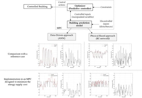
The purpose of this work is to combine these two types of analysis when the energy flexibility provided by the thermostatically controlled load can be also exploited. The two opposite modeling approaches (physical-based and data-driven) to predict the building energy demand are compared from two different points of view: (i) the capability of the models to reproduce the building energy behavior of a reference case and (ii) the practical implementation of a simple MPC designed to minimize the energy supply cost. In particular, the relationship between the model structure and its effectiveness in predicting the energy flexibility behavior will be explored.
With a dynamic cost tariff and the possibility of activating the building energy’s flexibility [
31] by allowing the indoor temperature to vary in a wider comfort range, the MPC can apply load shifting strategies to reach the goal. For the physical-based model, a lumped-capacitance model based on thermal–electrical analogy was used, while an ANN was chosen as data-driven model. The reference building, from which training data were extrapolated and in which the MPC was tested, was designed in a TRNSYS [
14] simulation environment. The goal was to highlight the advantages and disadvantages of the two approaches when they were implemented in an MPC.
After this introductive section,
Section 2 describes the methodology used to design the two models and the optimization process carried out by the MPC in the two cases. The case study is reported in
Section 3, while the results of the study are provided in
Section 4. The conclusions of the paper can be found in
Section 5.
2. Methodology
In this study, the goal of the MPC was to minimize the total energy cost for the building thermal demand satisfaction. The typical structure of an MPC is shown in
Figure 1. It is mainly composed of two parts: the building predictive model and the optimizer. The building predictive model should be able to dynamically forecast the building’s energy response in a certain period (prediction horizon,
ph), while its inputs can vary both in a controlled (manipulated variables) and in an uncontrolled (disturbances) way. To solve the optimization problem, it is important to define a proper objective function and to respect the system constraints; in this way, the optimizer has the possibility to select the best control actions to maximize the performance. Following a “receding horizon” logic, the MPC updates the best control action at each timestep, moving the prediction horizon forward and repeating the optimization [
5].
As anticipated, two different approaches for the building prediction model are used in this work: a data-driven model based on an ANN and a physical-based model with a thermal–electrical analogy structure. In order to obtain training data for the ANN and to check the MPC effectiveness, a detailed building model designed in TRNSYS [
14] was adopted as a control building.
The MPC routine was written in MATLAB [
32], and for each time step the controlled building started the MATLAB engine to run the controller. The uncontrolled inputs of the models were weather conditions and heat gains, while the manipulated variable was the hourly building energy demand. Since the objective of the work was to focus on the comparison between the two approaches for building modeling in an operative MPC, an ideal HVAC system was considered in the building, i.e., the thermal energy demand was treated as a control action (
Figure 1).
The optimizer solved the optimization problem in the prediction horizon,
ph, in order to minimize the total energy cost with constraints on the internal comfort conditions. As an incentive for the exploitation of the energy flexibility, a dynamic energy cost tariff was considered [
33]. In addition, to amplify the cost variations, a penalty signal was used in the MPC optimizer. It was obtained with a statistical method based on mean and standard deviation:
where
p is the penalty signal at each time
t,
c is the energy cost, while
μc and
σc are the cost signal mean value and standard deviation, respectively. Additional details about the penalty signal will be discussed in
Section 3.
The performance of each model was assessed by evaluating the root mean square error,
RMSE, which is defined as:
where
y is the variable being evaluated and
n is the number of points considered. Another index that will be used in the results is the root square error,
RSE, defined as:
The first analysis consisted of evaluating the deviation of the models with respect to the building reference data. Then, in order to assess the accuracy of the models in the operative MPC, the
RMSE was calculated between the prediction of the MPC building model and the actual thermal behavior of the building. Due to the different mathematical formulations of the two models, the optimization problem was different for the two cases. The following
Section 2.1 and
Section 2.2 discuss the mathematical formulations of the two approaches.
2.1. MPC with Physical-Based System Model
A lumped-parameter model based on the thermal–electrical analogy was chosen as the building prediction model in the physical-based MPC. The building thermal dynamics is represented by an equivalent circuit of thermal resistances and capacitances [
34]. A third order model was selected since it represented a good compromise between network complexity and capability of predicting the short-term dynamics of the building [
35].
As shown in
Figure 2, three thermal nodes were used. Each node is described by a temperature (
T) and a thermal capacitance (C). Then, four thermal resistances (R) were used to model the heat transfer between the nodes.
All the numerical values of the parameters (R and C) were deducted by the knowledge of the thermal and geometrical building features. Specifically, the first node (
Te, C
e) represents the external building thermal mass, the second node (
Tair, C
air) is the indoor air node, while the last node (
Ti, C
i) is the internal building thermal mass. As suggested by EN ISO 13790 [
36], C
e and C
i are calculated by summing the heat capacitances of all the building elements (up to the thermal insulation) in direct thermal contact with the internal air zone.
As concerns the thermal resistance, Rw is the thermal resistance from the indoor air node temperature to the ambient air temperature (Tamb), due to air changes and windows. Ree and Rie are the thermal resistances between the external building thermal mass node and Tamb and Tair, respectively. They are calculated as equivalent thermal resistances due to the conductive heat transfer of all the building envelope layers, from outdoor to the thermal insulation for Ree, and from thermal insulation to indoor for Rie. These thermal resistances also take into account the convective heat transfer phenomena between the external surface and ambient temperature (Ree) and between the internal building envelope surface and indoor air temperature (Rie). In the same fashion, Ri considers the thermal resistance between the indoor air node and the internal thermal mass Ti. The heat fluxes, directly applied to the internal thermal nodes Tair and Ti, are the cooling power derived by an ideal HVAC system (Q) and the total heat gains (G). The latter includes both solar and internal contributions, which are provided with a scalar factor (f) for both the internal air and the internal mass node.
The dynamics of the resistance–capacitance (RC) model can be represented by the following equations:
Using these relations, a discrete time invariant state–space formulation can be set up:
where [
X] = [
Tair Te Ti]
T represents the system state at each discrete time
k, [
U] = [
Tamb G Q]
T is the vector of the inputs, and [A] and [B] are coefficient matrices. A discrete time (
k) of 1 hour is adopted, as well as for the simulation time step (
t).
Along with the building prediction model, the MPC must include an optimizer. In the present work, the objective of the MPC was to minimize the total energy cost for the building thermal demand satisfaction while the indoor temperature remains in an allowed comfort range. For the physical-based MPC, a simple linear programming (LP) problem was formulated. In this optimization problem, both the objective function and constraints must be linear functions of the decision variables. The objective function (OF) is calculated as the sum of the building thermal energy consumption (
Qk) multiplied by the penalty signal
pk at each time step
k in the whole prediction horizon (
ph):
Therefore, the minimization problem can be written as:
subject to the following comfort and ideal HVAC constraints:
The LP optimization problem is solved at each time step within a MATLAB script, according to a “dual-simplex” algorithm. The actual air zone temperature,
Tair(
t), is passed to the MPC as the starting condition for the optimization. Based on the receding horizon principle, the control action at the controlled building time,
t, is the first value of
Qk in the optimal decision variable sequence. At the following time step,
t+1, the optimization problem is re-solved, moving forward the dataset of the disturbances by a time step.
Figure 3 shows the scheme of the operation.
2.2. MPC with Data-Driven System Model
The data-driven system used in the present study is based on an artificial neural network (ANN), a mathematical model that reflects the functioning of a biological brain [
37]. In an ANN, the inputs (
x) have the same role of biological dendrites, while the outputs (
y) can be regarded as biological axons. The processing of the data takes place in the neurons, which, in an ANN, apply a nonlinear activation function, g, on the input data. Being a pure mathematical model without physical meaning, an ANN needs to be trained with existing data. The purpose of the training, which can be carried out with different error minimization techniques, is to determine the coefficient weights and biases of the network, i.e., the parameters that fully describe an ANN. Taking into account a feedforward ANN consisting of only one layer of neurons (also called a hidden layer because its activation values are not directly accessible from outside the network) and a linear activation function in the output layer (with just one output), the mapping carried out by the ANN on the input can be expressed as follows:
where d is the number of inputs, w
ji is the weights matrix of the inputs, b is the bias vector of the inputs, m is the number of neurons in the hidden layer,
is the weights matrix of the hidden layer, and
is the bias vector of the hidden layer.
Generally, training data are divided into inputs and targets, and a well-trained ANN is expected to determine its outputs with a low deviation in respect to the provided targets. The available data of the system under study need to be examined carefully in order to train the ANN only with the inputs that most influence the objective targets. If the physics of the system under study is complex, a method to individuate the most effective inputs involves the use of statistical approaches such as factor analysis. Instead, if the physics of the system is not entirely unknown, the operator can try to select the input variables that mostly influence the desired target. In the present work, since the thermal behavior of the building is known, the four input variables (outdoor temperature, solar gains, internal gains, and indoor temperature) that most significantly influence the target variable (the thermal power required by the building) were selected.
The ANN was trained with 168 hourly-based input/target data referred to as a typical week. These data, provided by the building simulation environment designed in TRNSYS, were not obtained with a fixed set-point condition. In this case, in fact, the ANN’s performance would have been insignificant, as there would have been no correlation between the output and the controlled variable (the indoor temperature). Indeed, the control unlocks the energy flexibility of the building and allows indoor temperature variations in a given comfort range, as explained previously. Therefore, to improve the ANN’s prediction capability, the building simulation environment was allowed to work with multiple indoor set-point temperatures, varying within a reasonable comfort range. To avoid the overfitting of the data, i.e., an exaggerated interpolating behavior of the ANN, only a fraction of the dataset was actually used to train the network. Specifically, the initial dataset of 168 points was randomly divided into three subsets: a training set (60%), a validation set (20%), and a test set (20%). While the training data were used by the ANN to complete its training, the validation set was used as an internal interrupt criterium to end the training if overfitting occurred. The test set, instead, was used to evaluate the ANN’s performance after training, in order to check its prediction capability with new data.
ANNs are available in different architectures, based on the physical–mathematical problem that is being studied. In the present work, since the goal was to estimate the thermal power required by a building, a fitting ANN was chosen. In MATLAB, fitting ANNs have a feedforward architecture and are trained according to a Levenberg–Marquardt backpropagation algorithm, which uses regression analysis and
RMSE to evaluate the performance. As it is well-known that even one layer of neurons is sufficient to represent complex, nonlinear problems [
37], in this study, one hidden layer with five neurons was used. The neurons used a hyperbolic tangent sigmoid as activation function. The ANN therefore had the architecture as represented in
Figure 4.
After training, the ANN model was used in the MPC to predict the building’s thermal demand for a given prediction horizon,
ph. To this purpose, the ANN inputs were divided into uncontrolled (outdoor temperature, solar gains, and internal gains) and controlled (indoor temperature) variables (
Figure 1). In this way, it was possible to manipulate the ANN as a function of the indoor temperature and to carry out an optimization process in order to minimize the overall energy cost in the time period
ph. The objective function of the optimization algorithm can be therefore written as in Equation (8), subject to the constraints defined in Equations (10) and (11). Since the ANN function for the thermal demand was nonlinear, the optimization algorithm chosen in MATLAB was a programming solver based on the gradient method that uses an initial value for the indoor temperature as first attempt of solution. In the same fashion as the LP optimization problem defined for the physical-based model, the control action of the ANN-based MPC works according to the receding horizon principle (
Figure 3).
3. Case Study
For the case study, a detailed building model was implemented in TRNSYS using Type 56. The model was composed of a single thermal zone and the envelope characteristics were extrapolated by the Tabula Project [
38] for detached houses. The building was north-facing, while all the walls faced outwards and the floor was placed on the ground (considered at a constant temperature of 15 °C).
Table 1 reports the main geometrical and thermal properties of the building that was considered (a single family house), which were extrapolated by UNI-TR 11552:2014 [
39].
The structure was characterized by high levels of thermal insulation and double-glazed windows, which were air-filled, were selected (g-value of 0.7). An air change per hour (ACH) equal to 0.2 h
−1 was selected. Internal gains included occupancy and artificial lighting [
40]. The former was 120 W per person (occupancy density of 24 m
2 per person), while an artificial light density of 5 W m
−2 was considered (artificial light turns on if total horizontal radiation is less than 120 W m
−2 and turns off when the value exceeds 200 W m
−2). The building was located in Rome, Italy (41°55’ N, 12°31’ E), and a Meteonorm [
41] weather file was used as a typical meteorological year.
In this work, the cooling season was chosen for the MPC test. Analogous results, however, could have been obtained for the heating season. As mentioned in
Section 2, no specific HVAC system was modeled; instead, an ideal cooling control was used in Type 56 to extrapolate the training data [
14]. In this way, the MPC control actions were applied as convective heat gains to the air nodes (positive for heating and negative for cooling). An indoor air temperature range of 25–27 °C was chosen as the comfort condition (i.e.,
Tmin and
Tmax in Equation (10)) and a maximum cooling load power of 7 kW was fixed (i.e.,
Qmax in Equation (11)) [
42]. Since the cooling power was directly applied to the air-zone, the ideal HVAC can be compared to a traditional heat pump split system. Assuming an average COP of 2.5, the thermal energy requirement can be converted into electricity consumption, and the penalty signal can be obtained consequently (Equation (1)).
For the reference case, a fixed set-point of 26 °C was simulated in order to provide a comparison between the building as controlled with the MPC and without the MPC.
4. Results
As discussed in
Section 2, the evaluation of the forecast performance of the two building prediction models was realized according to two points of view: (i) the ability of the models to match the behavior of a known reference building and (ii) their dynamic operation when applied within the controller of the same building. Since short-term dynamics are involved in an MPC, a representative summer week was selected for the analysis (from July 30 to August 6).
Figure 5 shows the uncontrollable inputs in the selected period (i.e., ambient temperature and total gains).
As concerns the performance analysis, the ANN training data were selected as comparison terms to test the two building models. As mentioned in
Section 3, the ANN training data were obtained with daily random set-points, which could range in the allowed comfort band.
Figure 6 and
Figure 7 show the results in the entire 168-point dataset for the ANN-based model and the RC network, respectively. Since the output of the models was different in the two approaches, for the ANN the hourly cooling power forecasting was evaluated (
Figure 6a), while for the RC network the internal air node temperature was considered (
Figure 7a). As can be seen, both the prediction models were able to reply to the dynamic variations of the training data. In the first case, the
RMSE was 0.26 kW, while the value found for the RC network was 0.34 °C. As highlighted by the
RSE profile in
Figure 6b, for the ANN the deviation was mainly due to the inability of the network to simulate the cases with reduced or zero cooling demand. For the physical-based model, instead (
Figure 7b), there seemed to be a regular prediction error rather than specific peaks. It is worth noting that the
RSE assumes a maximum value of 0.9 °C in the RC model and a value of 0.8 kW in the ANN model.
When the building was allowed to be controlled by the MPC, at each time step the cooling power demand that was selected was the one that minimized the total energy cost. The original energy cost profile and its corresponding penalty signal in the representative summer week are shown in
Figure 8a,b, respectively. The use of the penalty signal, instead of the actual energy cost, allowed us to amplify the cost variation and, thus, to incentivize the unlocking of the building’s energy flexibility.
Figure 9 and
Figure 10 show the MPC results for both the prediction models. The results are presented with a prediction horizon,
ph, of 6 hours. Specifically,
Figure 9a and
Figure 10a show the comparison between the building’s actual internal air temperature (Type 56) and the MPC’s predicted value for the same time step (
t). Instead, in
Figure 9b and
Figure 10b, the control actions (
Q(
t) in
Figure 3) selected by the controller at each time step are represented. Looking at the black curves in
Figure 9a and
Figure 10a, it is possible to note that both the prediction models were able to activate the building’s energy flexibility, exploiting the whole comfort temperature range. Low temperature values are preferred when the energy cost is low and subsequent increases are expected. Conversely, the temperature is maintained close to the higher comfort range when high energy costs are detected.
The application of the MPC with both the prediction models produced a total cost reduction of about 16% if compared to the reference building with a fixed set-point of 26 °C. The RMSE between the actual air temperature and that predicted by the MPC at each time step also shows similar error values for the two models: 1.1 °C for the controller with the ANN and 0.99 °C for the RC model. However, comparing these values with the RMSEs found in the first part of the analysis, a degradation in the prediction performance can be noted for both the approaches. This is due to the fact that the building operated in variable dynamic conditions when the energy flexibility was activated. Thus, the predictions depend on constantly updated factors (such as the starting temperature conditions, the charge and discharge level of thermal inertia, etc.) which clearly amplify the prediction error.
Although the models seem to have similar performances, different on-time trends for the two models can be expected if the actual building air temperature is observed (the red curves in
Figure 9a and
Figure 10a). In particular, the MPC with the RC network seemed to follow the system dynamics more accurately than the controller with the ANN. When the ANN was operatively used in the controller, it appeared to perform less effectively than the RC network. In both cases, in the second half of the tested period, the prediction error started to grow but, in the case of the ANN, the actual air zone temperature exceeded the upper comfort limit by more than one degree (28.8 °C was the maximum value reached with the ANN in the controller, against 27.5 °C in the case of the RC model). This behavior is also confirmed by the duration curves reported in
Figure 11. In the building regulated by the ANN-based MPC, the indoor temperature was found to be above the upper control limit for 36% of the simulation time. This percentage dropped to 24% when the RC network was used. This behavior was due to the difficulty of the control to maintain the comfort level when the temperature was too close to the upper comfort boundary; a small error in prediction can also cause temperature violations.
In summary, a reversal of performance between the two models can be found when the evaluation is carried out for the application in a realistic controller. The main reason for this behavior is related to the difficulty in selecting the proper dataset for the ANN training. In fact, the model must not only be able to replicate the response of the building in the same input conditions (and this is done well in the present study), but it must also be able to predict the system’s responses in different scenarios, taking into account the contribution of energy flexibility. When the latter is introduced, it becomes difficult to identify a dataset that can train the black box model adequately, since the problem becomes dynamically affected by the operation of the system. Although the flexibility contribution seems to be better represented by the white box model based on the RC network, even in this case, a degradation in the prediction performance is detected when the controller is applied to the building. When using a white box model, however, a relevant amount of detailed data relating to the design and construction characteristics of the building should be known in order to implement an accurate model. Moreover, it is not always obvious which is the best network structure to use in the physical-based approach. For very complex buildings, it may be exceedingly difficult to identify an appropriate model and the corresponding parameters, even if detailed knowledge of the building is available. Another aspect that should be taken into account when using a purely physical-based model is that some dynamics (e.g., occupancy) cannot be considered in any way unless dedicated models are added. When, instead, measured data are used for the model training, such information may be intrinsically provided to the model. For these reasons, it could be convenient to monitor data and use hybrid models.
To conclude,
Table 2 reports a comparison summary between the two building model approaches, subdivided into the main steps of configuration and implementation in an MPC.
5. Conclusions
In this paper, a comparison between a data-driven model implemented with an artificial neural network (ANN) and a physical-based model realized with an RC network is provided in an operative model predictive control (MPC). The controller was designed to provide a minimization of the total energy cost for the thermal demand satisfaction.
Focusing on the evaluation of the cooling season, a 16% reduction in the weekly cost with respect to the reference case was obtained, with an RMSE of about 1 °C in both cases (1.1 °C with the data-driven model and 0.9 °C with the physical-based approach). Although the data-driven model shows a good performance in replicating the building’s thermal power profile, this trend is not confirmed when it works operatively in the controller. In fact, the comfort constraints are not respected for the 36% of the simulation time, with a maximum temperature deviation from the upper comfort limit of 1.8 °C. The physical-based model, instead, shows a discomfort percentage of 24% but a maximum deviation of only 0.5 °C.
The main conclusions of the presented work can be summarized as follows:
Both the controllers show a good ability to replicate the reference case behavior at equal inputs.
In the case of real implementation, for the ANN-based MPC, comfort constraint violations can occur more frequently. Indeed, the use of a data-driven model poses an issue for the training dataset to operatively represent the energy flexibility contribution in buildings.
The physical-based model seems to better reproduce the system dynamics. However, an accurate knowledge of the building, which is not always possible, is required.
Both the approaches show an amplification of the prediction error when their dynamic operation in the MPC is considered, even if the physical-based MPC limits this issue.
This latter point highlights the difficulty in implementing MPCs in real controls for energy flexible systems and suggests the need for further investigation. Indeed, it is important to consider that the results presented in this paper are related to a relatively simple building and no dedicated occupancy models were considered. When such advanced controls must be applied to more complex buildings where the role of users is not negligible, a purely physical-based approach can be computationally heavy, and it could be more convenient to use hybrid models. As a future development, it would be interesting to test the use of a hybrid model with an RC network structure and to provide a sensitivity analysis of the model according to the users’ behavior in order to assess whether improvements in operational performance are also evident in the case of a simplified building.


