Performance Evaluation of Control Methods for PV-Integrated Shading Devices

Abstract

This study aimed to develop a building-integrated photovoltaic (BIPV) device and optimal control methods that increase the photovoltaic (PV) efficiency and visual comfort of the indoor space. A louver-type PV-integrated shading device was suggested and an artificial neural networks (ANN) model was developed to predict PV electricity output, work plane illuminance, and daylight glare index (DGI). The slat tilt angle of the shading device was controlled to maximize PV electricity output based on three different strategies: one without visual comfort constraints, and the other two with visual comfort constraints: work plane illuminance and DGI. Optimal tilt angle was calculated using predictions of the ANN. Experiments were conducted to verify the system modeling and to evaluate the performance of the shading device. Experiment results revealed that the ANN model successfully predicted the PV output, work plane illuminance, and DGI. The PV-integrated shading device was more efficient in producing electricity than the conventional wall-mount PV systems, the control method without visual comfort constraints was most efficient in generating electricity than the other two with such constraints, and excluding the constraints resulted in less comfortable visual environment and reduced energy benefit. From the results analysis, it can be concluded that based on the accurate predictions, the PV-integrated shading device controlled using the proposed methods produced more electricity compared to the wall-mount counterpart.

1. Introduction

Solar power is one of the most promising, reliable, and environmentally friendly renewable energy technologies. It has the potential to significantly reduce reliance on fossil fuels, a resource that is quickly nearing exhaustion. Additionally, the substantial increase in the consumption of these fossil fuels has resulted in significant CO₂ emissions, accelerating the greenhouse effect which is the cause of global warming. To confront this issue, it is necessary to replace fossil fuels with renewable resources such as wind and solar energy and to develop strategies for the effective use of natural resources [1,2].

Photovoltaics (PV), which produce electricity using solar power, has become widely applied in buildings. The power conversion efficiency of PV systems has been continuously improved due to research on many aspects including materials and cells [3]. Emerging PV technologies include Perovskite cells, organic cells with various materials, and quantum dot cells [4,5,6,7,8]. Research-cell efficiency of non-concentrator setup reached 39.2% (multi-junction cells), 26.1% (single crystalline silicon) and 25.2% (Perovskite) in 2020 [9]. In particular, building integrated photovoltaic (BIPV) systems have increasingly been incorporated into elements of recent building enclosure systems. Building-integrated PV can provide sufficient energy for small-scale buildings while producing significant energy savings [10]. Furthermore, building-integrated PV systems can be installed at costs equal to that of many current façade cladding systems.

The advantages of BIPVs are significant, and, due to the potentially large benefits, more and more countries are starting to develop and construct BIPV systems on a large scale [11]. First, BIPV systems can be a cost-effective alternative energy source. According to Lin and Carlson [12], at peak power, a large-scale BIPV system has the potential to produce electricity at a cost comparable to that offered by a large, centralized power plant (less than 10 cents per kWh). They argue that as the cost of electricity storage keeps decreasing, a networked BIPV system could provide a reliable and cost-effective power source.

Besides the economic benefits, each kWp of PV installed as part of a BIPV system prevents the emission of approximately one ton of CO₂ per year [13]. The advantages of BIPVs are further enhanced when PV panels are effectively utilized for multiple functions within the building system. A BIPV system that functions as an adjustable shading device, for example, will produce electricity and also decrease building operational power usage by controlling solar heat gain through windows.

However, when PV panels are integrated into a building, factors such as aesthetics often compete with electricity production efficiency. Many BIPV systems operate below their maximum electricity production potential because of a sub-optimal orientation due to design constraints. PV panels vertically installed on a south wall presented a yearly average efficiency of 10.3%, 9.7%, 6.0%, and 5.9% for single crystalline silicon, multi-crystalline silicon, silicon film, and triple-junction amorphous silicon, respectively [14]. By contrast, the efficiency of single crystalline silicon and multi-crystalline silicon was 24.7% and 20.3% respectively in 2006 [15], and 26.7% and 22.3% in 2017 [16]. This indicates that BIPV systems often suffer from under-utilization of solar energy. It would be reasonable for BIPVs to take full advantages of solar cell technologies.

In addition, lack of shading control leads to occupant discomfort and waste of energy. In an office environment, worker comfort is of utmost importance in order to maximize productivity, and lighting conditions greatly influence occupant satisfaction. In addition, office workers prefer daylight to artificial lighting and desire easy access to the shading and lighting control systems that affect natural light transmittance [17]. Therefore, an automatic, easily accessible shading control system that considers daylight glare as well as illuminance is needed.

Few studies focus on the BIPV configured as an adjustable shading device. BIPVs have been investigated in many aspects: modeling and design methods [18,19,20], performance [21], application of semi-transparent solar cells integrated on windows [22,23], etc. Shading device control has also been widely studied, with a main focus on energy efficiency and occupant comfort [24,25,26]. However, the combination of BIPV and louver-type shading device requires further investigation, especially on control method and performance. This leads to the objective of this study.

The objective of this study is to propose a BIPV device and its control method that increase the efficiency and advance visual comfort. To achieve this objective, a PV-integrated shading device (PVIS) was suggested and the diverse control methods were comparatively tested to find the optimal control method.

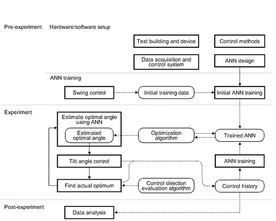
Figure 1 shows the research procedure. The first step was to develop artificial-neural-networks (ANN)-based optimal control methods for a PV-integrated shading system. Three control methods were developed: (i) PV-only method that adjusts the slat angle only for maximizing electricity production, (ii) PV + WP method that aims to maximize electricity production while maintaining the comfortable work plane, and (iii) PV + WP + DGI method that maximizes electricity production while keeping comfortable work plane and preventing daylight glare.

The second step was to develop a prototype motorized PV-integrated exterior louver with adjustable slat angles. As the slat angle is adjustable, a potential to produce more electricity as well as to provide a visually comfortable indoor environment exists. The third step was to setup the scale model for testing performance of each control method, in which PVIS, a wireless system for controlling motorized shading devices, sensors, and data acquisition systems, are installed. The last step was to test performance and analyze results in terms of electricity production and visual comfort. Results from three optimal control methods and the conventional wall-mounted PV device were comparatively analyzed. To summarize, this study aims to experimentally verify system modeling designed to optimize PV-integrated shading device performance.

2. Development of Control Methods

2.1. Factors Affecting PV Output, Illuminance, and Glare

The electricity output of the louver PV modules on a louver slat depends on solar availability, louver slat tilt angle, and the physical configuration of the louver. The factors affecting the solar radiation on a louver slat include sun position, sky condition, and reflectance of surrounding objects. The factors involving PV modules include PV efficiency, orientation, and PV coating fraction with regard to slat area. The PV module orientation depends on the slat tilt angle, which is the controlled variable in this study. The sky condition and the sun position are variables, but they are uncontrollable. The other factors are constants.

Visual comfort can be defined as a state of mind caused by the luminous environment perceived by human eyes. Several quantifiable and controllable factors can be used as general guidelines for the general population. These factors include the work plane illuminance and the daylight glare index (DGI), which are used to estimate visual comfort in this research.

The work plane illuminance depends on diverse factors. A louver, which comprises multiple horizontal slats, controls the daylight admission by the slat tilt angle. Therefore, the work plane illuminance depends on solar availability and the slat tilt angle of the louver. The solar availability depends on the sky condition and the sun position. Other factors affecting the work plane illuminance include the reflectance of interior surfaces, the room geometry, the transmittance of windows, the number and size of windows, and electric lighting. These factors remain constant in this research.

The daylight glare index (DGI) also depends on solar availability and louver slat tilt angle. The DGI equation considers four factors: window luminance, background luminance, window size subtended by an observer, and the viewing direction of the observer. The window luminance and the background luminance depend on the solar availability and slat tilt angle. The window size and the viewing direction are constants.

To summarize, the dependent variables are the PV electricity output, the work plane illuminance, and DGI. The independent variables affecting these dependent variables are the slat tilt angle, solar availability as estimated by exterior vertical illuminance, and sun position. The slat tilt angle is the only controlled variable. The other two variables are uncontrollable and thus measured or calculated. The other factors affecting the dependent variables are constants (see

Table 1. Variables and constants.

Types	Variables and Constants	Values
Design variables	Slat tilt angle Exterior illuminance Sun position	Controlled Measured Calculated
Dependent variables	PV electricity output Work plane illuminance Daylight glare index	Measured Measured Measured
Constants	Surface reflectance PV coating fraction Louver slat size and spacing Building geometry and location Window configuration Occupant position and viewing direction	(Constants)

).

2.2. Control Methods

Three optimal control methods were developed in this study. While they share an identical objective, maximizing PV electricity output, they have a different number and type of constraints. Depending on the criteria for optimization, three control methods were devised: (i) PV output only (PV-only), (ii) PV output and work plane illuminance (PV + WP), and (iii) PV output, work plane illuminance and daylight glare index (PV + WP + DGI).

The PV-only method, the first method, considered the electricity output from PV cells on the louver slats as the only criterion. The range of the slat angle was between −78 and +78 degrees. Thus, the optimization problem for maximizing PV output was subjected to the slat angle between −78 and +78 degrees. Since this method is used to achieve the maximum electricity output of the shading device, it is particularly useful when a space is unoccupied and attaining visual comfort is therefore unnecessary.

The PV + WP method, the second method, used two criteria: PV output and work plane illuminance. The control goal was to maximize PV output while maintaining the work plane illuminance above 500 lux. Keeping the work plane illuminance, which depends on available daylight, above 500 lux may be impossible regardless of slat tilt angles. In that case, the control goal was to maximize the work plane illuminance, because the work plane illuminance criterion has higher priority.

The PV + WP + DGI method, the third method, employed three criteria: PV output, work plane illuminance, and daylight glare. The control goal was to maximize PV output while keeping work plane illuminance above 500 lux and DGI below 22. When the work plane illuminance and DGI were both unacceptable, reducing DGI was the first goal.

2.3. Control Flow of the Slat Tilt Angle

One cycle of the optimal angle control in this study consists of two steps (see Figure 2). The first step, which was named logical global search, used ANN model for estimating an optimal louver slat tilt angle. The logical global search explored every possible combination of variables. For any given maximization problem, the combination with the highest objective function value is found after repeated comparisons between one combination and another.

Since the ANN model calculated the 53 candidate solutions for a single discrete variable which ranged between −78 and +78 degrees with a step size of three degrees, it is possible to perform a global search that yields a global optimum. Of the 53 sets of input variables, one that yields output variables closest to an optimum was selected. Because the tilt angle is a discrete variable, a higher PV output may occur at an angle between two discrete angles. As a result, the slat tilt angle was adjusted to the estimated optimal angle.

Artificial neural networks, which have often been used for building control and PV systems [27,28,29,30,31], were used to predict three output variables (louver PV output, work plane illuminance, and DGI) using four input variables: slat tilt angle, exterior illuminance, sun altitude and sun azimuth. Figure 3 shows the employed ANN model in this study. Initial input neurons were composed of four variables: louver slat tilt angle, exterior vertical illuminance, solar altitude, and solar azimuth. Additional variables that might increase ANN accuracy include solar profile angle, source luminance, and background luminance, which are functions of the four input variables. For this reason, they were excluded from the ANN. The output variables were louver PV output, work plane illuminance and DGI. The ANN was trained with the actual measurements.

The number of hidden layers and neurons in each hidden layer was designated as 2 and 5, respectively. The sigmoid function was employed as a transfer function for the hidden neurons and the pure linear transfer function was used for the output neurons. For the training of the ANN model, a 0.1—weighted-mean-squared-error goal, 10 million maximum iterations, 0.01—learning rate, and 0.9—momentum were applied. The configuration and learning methods of the ANN model were determined from the preliminarily conducted comparative performance tests on various ANN structures. For the ANN training, 28,822 training datasets were prepared during the pre-experiment period. The training period spanned ten hours (between 8 a.m. and 6 p.m.) of each day. Two of the four days were almost clear, and the other two days were rainy and partly cloudy, respectively.

The second step, which was named physical local search, employed a trial-and-error method to adjust the slat angle from the estimated optimum to an actual optimum by exploring adjacent angles. It tests whether a better solution exists by searching angles adjacent to the logical optimum estimated using an ANN. This test is necessary because there is no guarantee that the estimated optimum coincides with the physical optimum. In other words, the ANN-based estimated optimum is valid only within the model of inter-variable relations constructed in the ANN through training. In addition, the accuracy of the ANN should be evaluated by comparing it to the actual optimum. Only after the estimated optimum based on the ANN proves to be close to the actual optimum should the estimated optimum be used without correction using the trial-and-error control.

Figure 4 shows the process of trial-and-error control. The trial-and-error control starts by determining an initial control direction. When the current slat angle is in an infeasible domain, where any criterion is violated a direction that moves the angle toward a feasible domain is selected. For example, if the work plane illuminance is below 500 lux when the criterion is included in the control method (PV + WP or PV + WP + DGI), a direction increasing the work plane illuminance is selected. For the PV-only method, a tilt-down direction is selected because no constraints are present, and the ANN already estimates the current angle as an optimum. The physical angle adjustment can have opposite results. For example, the louver PV output can decrease after an angle adjustment for a higher PV output. Therefore, each adjustment is evaluated to check whether the adjustment coincides with the estimation. If the adjustment is incorrect, the opposite control direction is selected for consequent adjustments. Otherwise, the next angle in the current direction is checked. A variable, reverse count, is used to check the control termination conditions. It represents the number of incorrect control directions. After an incorrect control direction, the control direction is reversed, and the reverse count is incremented by one. Two incorrect directions followed by a final adjustment ends a trial-and-error control cycle.

At the beginning of a control cycle, a logical global optimum is acquired using the ANN. After the slat angle is adjusted to the estimated optimum, the trial-and-error control begins. These two processes can be described as a “physical local search starting at a logical global optimum.” The flow of slat angle control using two processes is shown in Figure 5. The trial-and-error starts at the estimated optimum, which serves as a best-guess initial angle for the physical search. Each angle adjustment is followed by a 10 s idle period for sensor data acquisition. Two measurements are acquired with an interval of 5 s during the period. The trial-and-error control terminates after the control direction is reversed twice. A control cycle terminates on the completion of the trial-and-error control. Each control cycle is followed by a 10 min idle period. During the idle period, the slat angle stays unchanged.

The error of the ANN is the difference between the estimated optimum and the actual optimum found by the trial-and-error control. This error is used to evaluate the accuracy of the ANN. Figure 6 illustrates the change of slat angle during an angle control cycle.

3. Development of the PV Device and the Scale Model

The performance of three optimal methods and one conventional wall-mounted PV method was experimentally tested in a scale model. Figure 7 shows the full-scale building and

Table 2. Features of the test module.

Building Related Components		Values
Location		Ann Arbor, Michigan, USA (42.289° N, 83.717° W)
Dimension	Real building 1/6 scale model	4.00 m wide × 6.00 m deep × 2.40 m high 0.67 m wide × 1.00 m deep × 0.40 m high
Window	Real building 1/6 scale model	3.40 m wide × 1.60 m high with no glass 0.57 m wide × 0.27 m high with no glass
Interior wall reflectance	Ceiling Walls Floor	65% 35% 13%

summarizes the major features of the building and module. The test building has an aperture located in the south wall. The window is 3.4 m wide and 1.6 m high. It has no glass. A 1/6 scale model of the building measuring 0.67 m wide, 1 m deep, and 0.4 m high was constructed and used for experiments. The test building and module were placed in Ann Arbor, Michigan, USA, located at approximately 42.289° north and 83.717° west. The interior ceiling, walls, and floor of the model were painted with semi-matte gray paints with a reflectance of 65%, 35%, and 13%, respectively. The reflectance of a surface was calculated by dividing the illuminance of the surface by that incident on the surface. The reflectance of each surface was determined by averaging 10 measurements.

A louver-type shading device was installed on the exterior of the south-facing window (see Figure 8a). The louver was assumed to have four horizontal slats with a spacing of 45 cm in the real building. The spacing was the same as the depth of a louver slat to allow the louver to thoroughly block the window. The louver slats were coated with polycrystalline PV cells, each of which were 6.6 cm wide and 3.6 cm deep (40 cm wide and 21.6 cm deep in actual size). To avoid low PV efficiency due to self-shading among louver slats, PV cells were installed only on the outer half (48%) of the slats. The other half (52%) was uncovered (see Figure 8b). Nine PV cells were attached to each louver slat and connected in parallel. A single cell was capable of a maximum of 8.0 V open circuit voltage with 44 mA short circuit current. The fill factor of the cell was approximately 0.65. Thus, one slat had a theoretical maximum power of 2.06 W. Considering the scale of the test building (1:6), the output power of the slat is equivalent to 74.1 W for a full-scale device. The total peak power of the full-scale device is 296.6 W (see

Table 3. Specifications of scale model and actual building.

Components	1/6 Scale Model	Real Building
Floor area	0.67 m2	24 m2
PV area per slat	196 cm2	7056 cm2
PV area (total)	784 cm2	28,224 cm2
Peak power per slat	2.06 W	74.1 W
Peak power (total)	8.24 W	296.6 W

).

Three major components were measured: PV output (electricity production), work plane illuminance, and DGI. Electricity production from PVs was measured using two groups of PV modules. One group was installed on the second-highest slat of the test louver. The other group was installed on the south wall of the test building. Because the open circuit voltage (V_OC) is almost constant during daytime, the short circuit current (I_SC) is measured to estimate the electricity output of PV cells. The PV output at the maximum power point (MPP) can be calculated using the fill factor, the ratio of MPP to V_OC × I_SC. The fill factor of the PV module used in the experiments was 0.65, according to its specifications.

Two types of light sensors were used to measure illuminance levels. Narrow range sensors (0–3630 lux) were used to measure work plane illuminance and background luminance [32]. The other wide-range type was for exterior light levels; it measures up to 230,000 lux. The wide-range light sensors were used for measurement points where a large dynamic range of light level was expected. Exterior daylight level was measured by a wide-range light sensor attached on the south wall.

DGI is calculated using background luminance, window luminance, and the solid angle of the window in relation to a hypothetical occupant. Hopkinson defines Daylight Glare Index (DGI) as the luminance of background and light sources, and the solid angle of the sources [33]. The definition is as follows:

$$\mathrm{DGI}=10{\log }_{10}{\displaystyle \sum }_{i=1}^n\frac{0.478L_i^{1.6}{\mathrm{\Omega }}_i^{0.8}}{L_b+0.07{\omega }_i^{0.5}{L}_i}$$

(1)

A modified equation based on Hopkinson’s equation is used. The test building has a single window. Therefore, no summing up procedure is necessary. The factors of i-th light source (L_i, ω_i, and Ω_i) are replaced with the factors of the single light source (L_s, ω, and Ω). The modified solid angle of the light source (Ω) is a function of the solid angle of the light source (ω) and the Guth’s position index p. The equation of the modified solid angle is

Ω = ω/p²

(2)

It was hypothesized that the occupant was facing toward the window, sitting at the center of the test building (three meters from the window). The eye level of the occupant was 1.2 m. The smallest possible value of p is 1, which occurs when an observer looks at the center of the light source. In other words, the line-of-sight coincides with the source-to-observer line. Therefore, Ω is always smaller than or equal to ω (Ω ≤ ω). In the modified equation, ω substitutes for Ω so that DGI represents the worst possible case. In sum, the modified DGI equation calculated the highest possible DGI of a single light source. The modified equation is as follows:

$$\mathrm{DGI}=10{\log }_{10}\frac{0.478L_s^{1.6}{\omega }^{0.8}}{L_b+0.07{\omega }^{0.5}{L}_s}$$

(3)

DGI values are interpreted based on the descriptive scale. The five thresholds in the scale define six states of daylight glare: non-perceptible (below 16), perceptible (16–20), acceptable (20–22), slightly uncomfortable (22–24), uncomfortable (24–28), and intolerable (over 28) [33]. When DGI is below the borderline between comfort and discomfort at 22, the daylight glare is considered acceptable.

Background luminance was the smaller of two luminance values measured near the left and right edges of the window (see Figure 9). Instead of the average of the two, the smaller value was used to represent the worst situation. Window luminance was calculated based on the illuminance measured using a shielded sensor. A circular area in the center of the window was used for window luminance measurement. Although it would be ideal to use the entire area of the window, it is difficult to precisely align a rectangular shield that confines the sensor’s field of view to the window. If the sensor is not precisely aligned, measurements are highly prone to errors. For this reason, the luminance of a partial area of the window was measured using a sensor with a circular shield. The solid angle of the circular area with regard to the shielded sensor was 0.02 sr. The window luminance sensor was calibrated using a commercial light meter.

In addition, the performance of a BIPV mounted on a south wall with the same PV area was estimated by comparatively analyzing the energy performance of a PVIS. Office buildings in the US consumed 72.9 kWh/m² (23.1 kBtu/ft²) for lighting in 2003 [34], 24.9% of their total energy consumption, which was 293.1 kWh/m² (92.9 kBtu/ft²). Based on this, a 24 m² office space consumes 4.79 kWh per day for artificial lighting. A south-facing vertical surface in Detroit receives, on average, 2.93 kWh/m² of irradiance per day [35]. When the conversion efficiency of a PV cell is 12%, a PV system mounted on a south-facing wall can produce 0.99 kWh, which is 20.1% of daily lighting energy consumption (see

Table 4. Estimated daily average electricity output from a wall-mounted photovoltaics (PV) system and lighting energy demand (climate data: Detroit, Michigan, USA).

Supply		Demand
PV area	2.82 m2	Floor area	24 m2
Orientation	South, vertical	Daily lighting energy per unit area	0.20 kWh/m2
PV efficiency 1	12%
Irradiance	2.93 kWh/m2/day	Total daily lighting energy	4.79 kWh
Electricity output	0.99 kWh/day

¹ Approximate.

).

4. Result Analysis

Test results in the scale model were analyzed to present the potentials of the developed control methods. For this, the prediction accuracy of the ANN model was investigated followed by the performance comparison between the optimal methods for PVIS and the conventional wall-mounted PV. In addition, each PVIS optimal control method comparatively investigated its PV-output efficiency, visual comfort, and energy saving effect.

4.1. ANN Prediction Accuracy

Figure 10 shows the ANN predictions for the PV output, work plane illuminance, and DGI for the clear sky conditions (March 25). Its prediction results were compared with those of actually measured sensor data. The average error of the ANN for the entire training period was 1.11 mA (PV output), 54.6 lux (work plane illuminance), and 0.868 (DGI). To capture the effect of outliers, rooted mean squared error (RMSE) was also examined; the ANN error was 1.71 mA, 94.1 lux, and 1.28.

In addition, the distribution of the ANN errors during the entire training period appears in Figure 11. Errors in most cases existed insignificantly. In total, 63.4% of PV output errors, 69.7% of work plane illuminance errors, and 72.7% of DGI errors were less than 1 mA, 50 lux, and 1, respectively.

The slat angle comparison between the estimated optimal angle from the ANN model and the actual angle is shown in Figure 12 and Figure 13 for each optimal method. For the PV-only method (Figure 12a), there were 47 cycles between 8:00 a.m. and 5:17 p.m. (9 h and 17 min) when the angle control was active. A cycle took 11.9 min on average. There were 378 step angle adjustments. There were 116 angle adjustments to the estimated optimum (30.7% of all angle adjustments). The other 262 adjustments (69.3%) were made by the trial-and-error control that moved the slat angle from the estimated optimum to the actual optimum. Every trial-and-error adjustment was made to increase the louver PV output; no other criteria were used. To increase the work plane illuminance, 120 adjustments were made.

The most frequently occurred slat angle error from the ANN model was three degrees; as much as 38.3% of the total cases, followed by 0 degree (21.3%), and 6 degrees (14.9%). Out of 47 cycles, the difference for 35 (74.5%) cycles was smaller than or equal to 6 degrees (Figure 13), which means that the ANN model predicted successfully the optimal slat angle. The average difference between the optimal angle acquired using the ANN and the actual optimal angle based on the trial-and-error control was 6.5 degrees. Because the goal of the trial-and-error control is to find an actual optimum starting at the ANN-based estimated optimum, the small average difference indicates the accuracy of the ANN.

Figure 12b and Figure 13 show the difference of slat angle between the estimated and the actual for the PV + WP method. There were 49 control cycles between 8:01 a.m. and 5:29 p.m. (9 h and 28 min), when the angle control was active. A cycle took 11.6 min on average (Figure 12b). There were 359 angle adjustments: 93 ANN-based adjustments and 266 trial-and-error adjustments. During the trial-and-error control, 146 adjustments were made to increase PV output when the work plane illuminance was above the acceptable level. To increase the work plane illuminance, 120 adjustments were made. For 41 of the 49 cycles (83.7%), the difference was less than or equal to 6 degrees (Figure 13). The average difference between the optimal angle acquired using the ANN and that acquired using trial-and-error was 4.9 degrees for the PV + WP method.

For the PV + WP + DGI method, there were 47 control cycles between 8:00 a.m. and 5:12 p.m. (9 h and 12 min) when the angle control was active (Figure 12c). A cycle took 11.7 min on average. The slat tilt angle was adjusted 356 times; there were 98 ANN-based adjustments and 258 trial-and-error adjustments. During the trial-and-error control, 131 adjustments were made to increase PV output when the work plane illuminance was above the acceptable level. To increase the work plane illuminance, 127 adjustments were made. No adjustments were made to decrease DGI because it stayed within the acceptable range. In 37 out of 47 cycles (78.7%), the difference between the estimated optimal angle and the actual one was smaller than or equal to 6 degrees (Figure 13). The average difference between the predicted optimal angle and the actual optimal angle was 4.5 degrees.

4.2. Three PVIS Optimal Methods Versus the Wall-Mounted Method

The PV output results of each optimal method were compared with those of the conventional wall-mounted method in Figure 14. The experiment day, when the PV-only method and the wall-mounted method were tested, was cloudy in the morning and almost clear in the afternoon. The exterior vertical illuminance indicating the daylight availability fluctuated between 9:30 a.m. and 12:00 p.m. Thus, the PV output fluctuated in the morning as shown in Figure 14a.

The average electric current of the louver PV between 8 a.m. and 6 p.m. was 17.25 mA, while that of the wall PV was 12.46 mA. The louver PV generated 38.4% more electricity than the wall PV. During the latter period (4 h) when the solar access was stable, the average electric current of the louver PV and the wall PV was 24.65 mA and 16.66 mA, respectively. The louver PV generated 47.9% more electricity than the wall PV. These results demonstrate that PV panels installed on louvers can generate almost 50% more electricity than those mounted on south-facing walls on a clear day in spring and fall. Because PV output depends on sunlight incident angle, this difference varies according to the sun position. It increases during summer, when the solar incident angle on the south wall is greater than that on the louver tilted perpendicularly to the sunlight profile angle. The difference during winter is smaller than that during spring and fall for the same reason. The sunlight incident angle on the louver could have been decreased further, but the combined effect of the direct and the indirect components of daylight caused the maximum PV output to occur at a slat angle lower than one minimizing the solar incident angle.

In Figure 14b, the output results of the PV + WP method, which sought to prevent unacceptable light levels by including work plane illuminance as a control criterion in addition to electricity output from the PV cells, were compared with those of the wall-mounted method. For the PV + WP method, the average electric current of the louver PV was 15.70 mA, which was 16.5% higher than that of the wall PV, 13.48 mA. Between 12:37 p.m. and 4:37 p.m. (four hours after the solar noon), the average electric current of the louver PV and the wall PV was 22.74 mA and 16.87 mA, respectively. The louver PV produced 34.8% more electricity output than the wall PV.

The ratio of the louver PV output to the wall PV output was 13.1% lower, in terms of the wall PV output, than that of the PV-only method. The PV output was lower because the louver angles were adjusted not only for PV electricity output but also for work plane illuminance. The work plane illuminance criterion caused the slat angle to be tilted up from the maximum PV output angle, maintaining the work plane illuminance at the acceptable level.

The results of the PV + WP + DGI method were compared in Figure 14c. In this control method, the daylight glare estimated by DGI had the highest priority. In other words, the controller attempted to lower DGI when it was greater than 22. The work plane illuminance had the second-highest priority. Only after these two criteria were satisfied did the controller attempt to maximize the louver PV output. As the DGI constraint remained inactive (DGI < 22), the results were identical to those of the PV + WP method. The average electric current from the louver PV (15.78 mA) was 17.8% higher than that from the wall PV (13.40 mA) between 8 a.m. and 6 p.m. During the four hours after the solar noon, 12:37 p.m.–4:37 p.m., the average electric current of the louver PV and the wall PV was 23.46 mA and 17.31 mA, respectively. The louver PV’s electric current was 35.6% higher than the wall PV’s. These values (17.8% and 35.6%) are consistent with the corresponding values from the PV + WP method (16.5% and 34.8%).

4.3. Performance Comparison of Three PVIS Optimal Control Methods

The effect of the work plane illuminance constraint can be assessed by comparing the PV-only method, the PV + WP, and the PV + WP + DGI methods. The comparison is based on the four hours after the solar noon (12:37 p.m.–4:37 p.m.), given as the gray area in Figure 15 to exclude from consideration most of the erroneous data and daylight fluctuation. The louver PV output was normalized using the wall PV output for comparison. Adopting the work plane illuminance constraint caused the normalized ratio of the louver PV to the wall PV to decrease from 1.48 (PV-only method) to 1.35 (PV + WP method) and 1.36 (PV + WP + DGI method). The decrease was 8.8% and 8.4%, respectively.

As summarized in

Table 5. Distribution of work plane illuminance and DGI.

Visual Comfort Components		Demand
		PV-Only	PV + WP	PV + WP + DGI
Work plane illuminane (lux)	0–350 350–400 400–450 450–500 500–550 550–600	69 27 4 0 0 0	<1 <1 2 25 70 2	<1 <1 <1 32 67 <1
DGI	0–14 14–16 16–18 18–20 20–22	0 51 34 15 0	0 58 18 24 0	<1 53 22 25 0

, using the work plane illuminance criterion maintained the work plane illuminance at acceptable levels. In contrast, using the PV-only method, which excluded the daylight criterion, resulted in unacceptable light levels on the work plane. The average work plane illuminance of the PV-only method, the PV + WP method, and the PV + WP + DGI method was 300, 504, and 505 lux, respectively. For the PV-only method, the work plane illuminance was below 450 lux for the entire comparison period; it fell below 350 lux for 69% of the period. For the remaining 31% of the period, it was either between 350 and 400 lux (27% of the period) or between 400 and 450 lux (4% of the period). In contrast, using the other two methods (PV + WP and PV + WP + DGI), both of which include the work plane illuminance constraint, resulted in values above 500 lux for 72% and 67% of the period, respectively. In addition, the work plane illuminance of the two methods was above 450 lux for most of the comparison period (97% of the period for PV + WP and 99% for PV + WP + DGI).

DGI remained within the comfortable range for every control method tested as summarized in Table 5. When DGI is below 22, the threshold between comfort and discomfort, daylight glare is considered acceptable. During the experiments, all DGI values were below 20. For more than half of the experiment period, the daylight glare was deemed non-perceptible (DGI greater than 16 was considered perceptible). The duration of non-perceptible daylight glare for the PV-only method, the PV + WP method, and the PV + WP + DGI method was 51%, 58%, and 53%, respectively. In the other cases, DGI was perceptible and acceptable (between 16 and 20).

The energy saving benefit of the PV + WP method is greater than that of the PV-only method. The total energy saving is the sum of PV electricity output and the reduction in electric lighting energy. For the PV-only method, the daily electricity output from the louver PV modules was 1.38 kWh/day, which is 28.8% of the test building’s estimated lighting energy demand, 4.8 kWh/day (see Table 4). Because the work plane illuminance was below the acceptable level, there was no electricity saving from reducing artificial lighting.

The electricity output was calculated based on the output of a single PV module of the scale model. The electricity output of the module after the solar noon was 532.6 mWh. Because the output before the solar noon fluctuated, this period was not considered for comparison. The output was based on the PV output current measured every 5 s, the open circuit voltage (8 V), and the fill factor of the PV module (0.65). The fill factor refers to the ratio of the maximum power of a PV module to the open circuit voltage (V_OC) multiplied by the short circuit current (I_SC). Therefore, for the PV-only method, the output of a single PV module on April 5 afternoon was estimated as 1.07 Wh under a clear sky. After applying the total number of PV modules (36), the scale to the real building (1:6) to the PV output of the scale model, the PV output of a full-scale building 1.38 kWh/day was acquired. The wall PV output of the full-scale building on the same period was 0.92 kWh.

For the PV + WP method, the energy saving was at least 1.91 kWh/day: 1.25 kWh from the louver PV modules and 0.66 kWh from electric lighting energy reduction. The total energy savings represented 39.7% of the test building’s daily lighting energy demand. The duration of the work plane illuminance above 500 lux was used instead of the duration above 450 lux (7.9 h). Because the work plane was in the center of the room, the lighting energy saving for the southern half closer to the window was considered. In addition, the lighting energy demand was assumed to be evenly distributed throughout the day. This assumption was used to avoid overestimating the electric lighting energy savings. Therefore, the energy conservation from natural lighting was at least 0.66 kWh (6.6 h/24 h × 12 m² × 0.2 kWh/m²). The energy saving of the PV + WP + DGI method was 1.88 kWh (39.3% of daily lighting energy demand).

As discussed above, the total energy benefit of the control methods with the work plane illuminance criterion was greater than that of the method without it. Although the PV outputs of the PV + WP method and the PV + WP + DGI method were lower than that of the PV-only method, their energy savings from natural lighting led to higher overall energy savings. The daylight glare stayed within the comfort range, ensuring that the louver could be automatically controlled without the occupants manually overriding it in an attempt to reduce visual strain.

5. Conclusions

This study aimed at developing a BIPV device and optimal control methods that increase the PV efficiency and visual comfort of the indoor space. A PV-integrated shading device (PVIS) was suggested and an ANN model were developed to predict PV output, work plane illuminance, and daylight glare index (DGI). Using the predicted values, three PVIS control methods including PV-only method, PV + work plane illuminance (PV + WP) method, and PV + work plane illuminance + daylight glare index (PV + WP + DGI) method were developed for controlling the louver slat angle and their performance was experimentally tested in the scale model. Test results revealed that the ANN model successfully predicted the PV output, work plane illuminance, and DGI; three PVIS methods were more efficient to produce electricity than the conventional wall-mounted method; the PV-only method was most efficient to generate electricity than the other two PVIS methods; and the PV-only method provided less comfortable visual environment and energy benefit. From the results analysis, it can be concluded that based on the accurate ANN predictions, three PVIS optimal control methods produced more electricity compared to the conventional wall-mount PV method. In addition, although the PV outputs of the PV + WP method and the PV + WP + DGI method were lower than that of the PV-only method, their energy savings from natural lighting led to higher overall energy savings.

This study aimed at proposing a BIPV device and optimal control method that increases the PV efficiency, maintaining visual comfort. A PV-integrated shading device (PVIS) is suggested and the diverse control methods are comparatively tested to suggest the optimal control method. An ANN model and three PVIS control methods, which employed the ANN model, were developed and comparatively tested their performance in terms of electricity production efficiency, work plane illuminance, and DGI using experiments in the scale model. Findings from the result analysis:

(1)

The ANN model predicted the PV output, work plane illuminance, and DGI accurately enough to be actually applied. The average error was 1.11 mA (PV output), 54.6 lux (work plane illuminance), and 0.868 (DGI). Rooted mean squared error (RMSE) was also examined and was 1.71 mA, 94.1 lux, and 1.28. Errors in most cases existed insignificantly: 63.4% of PV output errors, 69.7% of work plane illuminance errors, and 72.7% of DGI errors were less than 1 mA, 50 lux, and 1, respectively.

(2)

The logical global search process using ANN model successfully found the optimal slat angle of the louver. The average of difference between the estimated angle based on the ANN model and the actual optimum angle was 6.5, 4.9, and 4.5 degrees for the PV-only, PV + WP, and PV + WP + DGI method, respectively. Over, 74.5%, 83.7%, and 78.7% of cases of each method were less than or equal to 6 degrees.

(3)

PVIS methods were more efficient to produce electricity. Compared to the conventional wall-mounted PV method, the PVIS methods generated more electricity as much as 47.9% (PV-only), 34.8% (PV + WP) and 35.6% (PV + WP + DGI).

(4)

Among the three PVIS optimal control methods, the PV-only method was most efficient to generate electricity because the only target of the PV-only method was to increase electricity output. The normalized ratio of the louver PV to the wall PV was 1.48 (PV-only), 1.35 (PV + WP), and 1.36 (PV + WP + DGI), respectively.

(5)

The PV-only method, however, provided an uncomfortable visual environment more than the other two optimal methods. The work plane illuminance by the PV-only method was below 450 lux for the entire comparison period. In contrast, using the other two methods (PV + WP and PV + WP + DGI) conditioned the work plane illuminance above 500 lux for 72% and 67% of the period, respectively.

(6)

The total energy benefit of the control methods with the work plane illuminance criterion was greater than that of the method without it. The energy saving benefit of the PV + WP and the PV + WP + DGI methods was at least 1.91 kWh and 1.88 kWh for about the four hours, respectively. These results are also summarized in

Table 6. Summary of PV-integrated shading device (PVIS) control methods.

	Control Method
	PV-Only	PV + WP	PV + WP + DGI
Objective	Maximize PV electricity output	←	←
Visual comfort constraints	None	Work plane illuminance	Work plane illuminance and daylight glare
Ratio of electricity out to wall-mount PV	1.48	1.35	1.36
Advantages	PV electricity output	Visual comfort	Visual comfort
Disadvantages	Visual comfort not guaranteed	Decrease in PV electricity output Uncomfortable daylight glare may occur	Decrease in PV electricity output

.

From the results analysis, it can be concluded that the ANN model successfully predicted the PV output, work plane illuminance, and DGI. Based on the prediction results, three PVIS optimal control methods produced more electricity compared to the conventional wall-mount PV systems. In addition, although the PV outputs of the PV + WP method and the PV + WP + DGI method were lower than that of the PV-only method, their energy savings from natural lighting led to higher overall energy savings.

Overall, in this study, limited conditions were used for performance testing in the scale model. Thus, comprehensive performance tests in the actual building and in the numerical simulation method should be conducted in further studies to ensure applicability.