Model of R134a Liquid–Vapor Two-Phase Heat Transfer Coefficient for Pulsating Flow Boiling in an Evaporator Using Response Surface Methodology

Abstract

The present study proposes a model to predict the heat transfer coefficient in R134a liquid–vapor two-phase pulsating flow boiling in an evaporator using the experimental data and response surface methodology (RSM). The model is based on the current existing empirical correlation for R134a liquid–vapor two-phase continuous flow with an imposed modification factor. The model for the imposed modification factor is the function of the pulsating period and inlet/outlet vapor quality, which is obtained using the limited experimental data. An analysis of variance (ANOVA) is carried out to test the significance of the model and normal probability of residuals is analyzed as well. Results show that the regression model produces a mean error of −4.3% and a standard deviation of 15.4%, compared to experimental results. Of the data 95.1% is contained inside a ±50% error window, which indicates that the proposed model could predict the heat transfer coefficient of R134a liquid–vapor two-phase pulsating flow boiling well.

1. Introduction

Numerous strategies, including passive and active techniques such as a fin-tube, coiled wires, and swirl/pulsating flow generator are widely used to improve the thermal performance of heat exchangers [1,2,3]. Pulsating flow (pulsed flow), characterized as the periodic change of one or some flow parameters, occurs in numerous systems (refrigeration, chemical engineering, etc.), and has a special significance in the operation of modern industrial equipment technologies. Studies on pulsating flow in a heat exchanger are essential because they are beneficial to understanding flow characteristics and improve heat transfer performance. To date, heat transfer characteristics in pulsating flow have been investigated previously by many researchers with conflicting conclusions, especially for the liquid–vapor two-phase flow [4,5,6].

Different from the single-phase flow, the two-phase heat transfer coefficient (HTC) predictions require not only a broad, accurate experimental database, but also a good knowledge of the heat transfer mechanism. For this purpose, many research proposed different empirical correlations to predict the HTC in the two-phase flow. One classical type is based on the HTC of liquid flow with Dittus and Bolter correlation [7] and on some dimensionless numbers (boiling number Bo, convective number Co, Froude number Fr, Martinelli parameter X_tt, etc.), which can be usually written as follows:

$$h_{\mathrm{tp}}=h_l·f(Bo,Fr,X_{\mathrm{tt}},\dots )$$

(1)

Shah presented a correlation by considering the nucleate boiling component and the forced convection component, and selected the larger of the two components [8]. Saiz Jabardo et al. proposed a correlation that is related to Bo, Fr, and X_tt [9]. The models of Chaddock and Buzard [10], Wattelet et al. [11], and Panek [12] mainly are the functions of X_tt. The second category is the power-type multiplication model for two boiling components that is analogous to the Dittus–Boelter correlation, and also can be written as:

$$h_{\mathrm{tp}}=Af({Re}_l^{C1},B{\mathrm{o}}^{C2},W{\mathrm{e}}_l{}^{C3},x,\dots )$$

(2)

where A is the area of the cross section. Tran et al. carried out R12 flow boiling transfer experiments in small channels and proposed a correlation with a function of Bo, We_l, and ρ_l/ρ_g [13]. Kew and Cornwell [14] observed an increase of HTC with the vapor quality in larger tubes and modified the Lazarek and Black’s correlation [15]. In term of application, these two categories of correlations are simple as they do not require the identification of the flow pattern. However, Silva Lima et al. conducted an experimental study on flow boiling in a horizontal smooth tube for R134a, and found the correlation above mentioned tended to underpredict the experimental results [16]. Mikielewicz presented a new method for flow boiling HTC in both conventional channels and minichannels by the hypothesis that energy dissipation resulting from the friction is linked to the heat transfer in the flow boiling process [17]. By the analyses for various experimental investigations in flow boiling, it is found that both the convective and nucleate boiling heat transfer mechanism played import roles in the two-phase heat transfer process [18]. The third format usually can be written as:

$$h_{\mathrm{tp}}={({(S{h}_{\mathrm{pool}})}^n+{(F{h}_l)}^n)}^{1/n}$$

(3)

where n is the power of number. The factor S (suppression factor, <1) reflects a lower effective superheat available in forced convection, which is opposed to pool boiling [19], because of the thinner boundary layer. The factor F (>1) indicates that much higher velocities could enhance forced convection heat transfer for the two-phase flow compared to the single-phase fluid flow. Gungor and Winterton assumed that the convective and nucleate boiling heat transfer have the same effect, and presented a general correlation for forced convection boiling in tubes and annuli with n = 1 [20]. However, they pointed that the HTC was overpredicted for the high vapor quality and underpredicted for the low quality [21]. It indicates that the simple superposition of the two heat transfer mechanism is not suitable. Therefore, Liu et al. modified the superposition relationship of nucleate boiling heat transfer and forced convection heat transfer in the form of the square root [22]. Based on superposition methods and considering the flow pattern characteristics, Kattan et al. proposed a flow pattern based method to develop the correlation [23]. The assumption of the linear variation of the dry angle without the consideration of flow patterns leads to the underprediction at low vapor quality. Subsequently, Wojtan updated the calculation of dry angle for slug flow, stratified-wavy flow and slug-stratified wavy flow to avoid any jump in HTC at any transition boundary and modified Kattan’s correlation [24].

According to the research results from the literatures, heat transfer in two-phase flow boiling is very complex, and related to many parameters such as the mass flow rate, heat flux, vapor quality, flow pattern, even fluid properties, and so on. Results show the different HTC correlations in flow boiling have different accuracy for different working conditions. It should be noted that all the correlations above are developed for the liquid–vapor two-phase continuous flow. The introduction of pulsating flow would further increase the complexity of two phase flow boiling as the flow, the liquid–vapor interface and flow pattern is always dynamic instead of a fully developed state in continuous flow. In our previous study, the heat transfer in two-phase pulsating flow is strongly affected by the pulsation period, mass flux, and vapor quality. Additionally, the heat transfer enhancement mechanism of heat transfer is the change of the liquid–vapor interface and wetted wall caused by the flow regime transition [25,26]. To the best of our knowledge, few literatures are devoted to obtain the HTC model for the two-phase pulsating flow. Besides, the correlation of the heat transfer coefficient in the two-phase flow needs a large database with a huge number of experiments. Response surface methodology (RSM) can obtain the regression equation of factors and responses by limited experimental designs and both considering the interaction relationship between factors. Therefore, the main objective of this study is to develop an HTC model for the two-phase pulsating flow based on the current experimental data and RSM.

In this work, a model has been proposed to predict HTC for the R134a liquid–vapor two-phase pulsating flow. In this model, the HTC in the two-phase pulsating flow is predicted using the HTC in continuous flow multiplied by a ratio factor. The ratio factor is the function of the pulsating period, mass flux, and vapor quality. One hundred and sixty experimental data under a variable mass flux, pulsating period, and vapor quality are used as the data base and processed with RSM to obtain the ratio factor of HTC of pulsating flow to that of continuous flow. Although the model is based on limited experimental data, it provides a simple tool to predict heat transfer of the pulsating flow, which could be extremely valuable for the pulsating system design.

2. Experimental Approach, Test Conditions, and Data Source

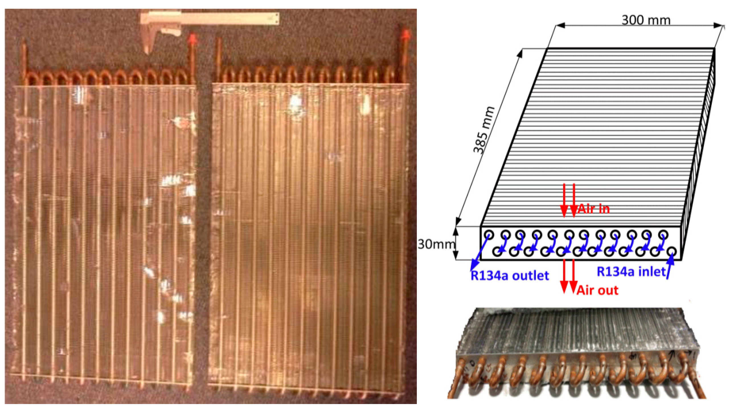
2.1. Pulsating Flow Boiling Facility

Pulsating flow is always generated by the nature of system or flow instability, which is not controlled. In our experiment, the flow is pulsed with a setting period controlled by a solenoid valve. For the comparison of both continuous flow and pulsating flow, two identical loops with two identical evaporators (HX1 and HX2, see Figure 1) were created. For the continuous flow, one of solenoid valves keeps open and other is closed, a continuous flow enters one evaporator exchanging heat with ambient air. For the pulsating flow, the two solenoid valves alternately open and close with a periodic time setting (when one solenoid valve opens the other was closed, and vice versa). In this way, the flow through the evaporators is pulsed, and is steady outside the evaporators. Therefore, the two loops are never closed simultaneously when pulsation occurs, which could ensure a steady state inlet pressure and a continuous mass flux before the evaporator.

Figure 1. The pulsating flow boiling test facility schematic.

Figure 1 shows a schematic of the two-phase pulsating flow boiling experimental system [25,26]. There are three loops in the system: refrigerant loop (red line), air loop (orange line), and chilled loop (blue line). In the refrigerant loop, the subcooled refrigerant R134a is pumped by a gear pump from a subcooler. Then the fluid passes through a flow meter and is heated by a pre-heater to control the vapor quality before the evaporators. After that, the two-phase R134a enters the two same sub-loops, starting from the solenoid valves, then the heat exchangers (HX1 and HX2), where it exchanges heat with air flow in a wind tunnel. After the heat exchanger, R134a is heated into superheated vapor by the superheaters. Finally, the two sub-loops meet and the vapor passes the condenser and is cooled by a chilled system. The heat exchanger used in our experiment was the fin-tube heat exchanger with 385 mm × 300 mm × 30 mm (length × width × thickness). The inner diameter of copper tube was 6.2 mm. The plain aluminum fins had a fin density of 15 fpi and fin thickness of 0.3 mm. The heat exchanger is shown in Figure 2.

Figure 2. Photo of the heat exchanger.

The chilled loop is used to cool the refrigerant vapor in the condenser and subcooler. The chilled fluid is the mixture of water and ethylene glycol with a volume ratio of 1:1. The temperature of chilled fluid is measured before and after the condenser. The air loop provides air flow to exchange heat with two-phase R134a in the heat exchangers. The air flow rate is measured by a nozzle system. The measurement method and design of the nozzle refer to the American Society of Mechanical Engineers (ASME) Standard MFC-3M [27] and ASME Standard PTC 19.5 [28]. The air flow is circulated by a blower controlled by a speed controller. The temperature of the air flow is measured before and after the heat exchangers.

2.2. Test Conditions and Data Reduction

The experiments were designed to ensure that HTC could be evaluated only under conditions of the liquid–vapor two-phase flow in the heat exchanger tubes. To be specific, the vapor quality at the inlet of the evaporator is controlled by adjusting the input power of the preheater according to the mass flow rate. The product of the refrigerant mass flow rate multiplying the enthalpy difference before and after the preheater is used to estimate the input power of the preheater. The outlet vapor quality is controlled by adjusting the air flow rate and the input power of the superheater. Additionally the product of the refrigerant mass flow rate multiplying the enthalpy difference before and after the superheater was used to estimate the input power of the superheater. The matrix of the experimental design is given in Table 1.

Table 1. Experimental matrix.

Variables	Refrigerant Side	Air Side
Flow rate	Continuous flow: 75–250 kg/(m2·s)	0.8–8.0 m/s
	Pulsating flow: double
Temperature	Evaporation Temperature: 15 °C	Inlet Temperature: 25 °C
	Superheat Temperature: 35–40 °C	(room temperature)
Vapor quality	Inlet of heat exchanger: 0.1–0.4	-
	Outlet of heat exchanger: 0.6–0.9
Operating mode	Continuous flow	Continuous flow
	Pulsating flow: period 2–24 s

The meausred parameters before and after the evaporator (HX) is shown in Figure 3. The air inlet/outlet temperature and flow rate were measured to calculate the heat exchange (q_a) at the air side as shown in Equation (4). The refrigerant mass flux (m_a), subcooling temperature (T_ri) before the preheater, the power of the preheater (q_hin) and the super heater (q_hsup), and the superheat temperature (T_rsup) after the superheater were measured to calculate the heat exchange (q_r) at the refrigerant side as shown in Equation (5). The overall heat transfer coefficient U was calculated based on the average heat transfer rate q_ave using the LMTD method, as shown in Equation (7). Finally the refrigerant side heat transfer coefficient h_r was derived by subtracting the thermal resistance of air side and wall heat conduction.

$$q_{\mathrm{a}}=m_{\mathrm{a}}{c}_p{}_{\mathrm{a}}(T_{\mathrm{ao}}-T_{\mathrm{ai}})$$

(4)

$$q_{\mathrm{r}}=m_{\mathrm{r}}(h_{\mathrm{rsup}}-h_{\mathrm{ri}})-q_{\mathrm{hin}}-q_{\mathrm{hsup}}$$

(5)

$$q_{\mathrm{ave}}=\frac{q_{\mathrm{a}}+q_{\mathrm{r}}}{2}$$

(6)

$$\frac{1}{U{A}_i}=\frac{1}{h_{\mathrm{r}}{A}_i}+\frac{1n(r_o/r_i)}{2\pi kL}+\frac{1}{\eta h_{\mathrm{a}}{A}_o}$$

(7)

where h_ri and h_rsup are the enthalpy of the refrigerant before the preheater and after the superheater. h_r and h_a are the refrigerant and air side HTC. r_o and r_i are the inner and outer diameter of the tube. A_o is the heat transfer ares of air side. η is the fin efficiency. Additionally, h_a is calculated using correlation Kim–Youn–Webb’s correlation [29].

Figure 3. Measured parameters for data reduction.

The sensors, ranges, and accuracy of the measured parameters are listed in Table 2. The measurement accuracy caused an averaged error of ±10.4% for the overall HTC, and ±12%–±16.5% for the refrigerant side HTC. More detail about the experimental approach, test conditions, and data source can be found in our prior work [25,26].

Table 2. Sensors, ranges, and accuracy of measured parameters.

Heat Transfer Side	Measured Parameters/Unit	Sensors	Range	Accuracy
Air side	Temperature/°C	Copper-constantan T type	−10–80	±0.1/°C
	Pressure drop/kPa	Setra Model 264	0–0.623	±1% FS
Refrigerant side	Mass flow rate/(g/s)	Micromotion DS006S	0–18	±0.1% RS
	Pressure (inlet of HX)/kPa	Sensotec Model Z	0–1034	±0.25% RS
	Pressure (outlet of HX)/kPa	Sensotec Model TJE	0–689	±0.25% RS
	Temperature/°C	Copper-constantan T type	−10–80	±0.1/°C
	Pressure drop/kPa	Rosemount 1151DP4E2A	0–37.36	±0.25% RS
	Heat power/W	AC Watt Transducer PC5	0–1000	±0.02 W
	Overall HTC/W·m−2·K−1			±10.4%
	Refrigerant side HTC/W·m−2·K−1			±12%~±16.5%

3. Results and Discussions

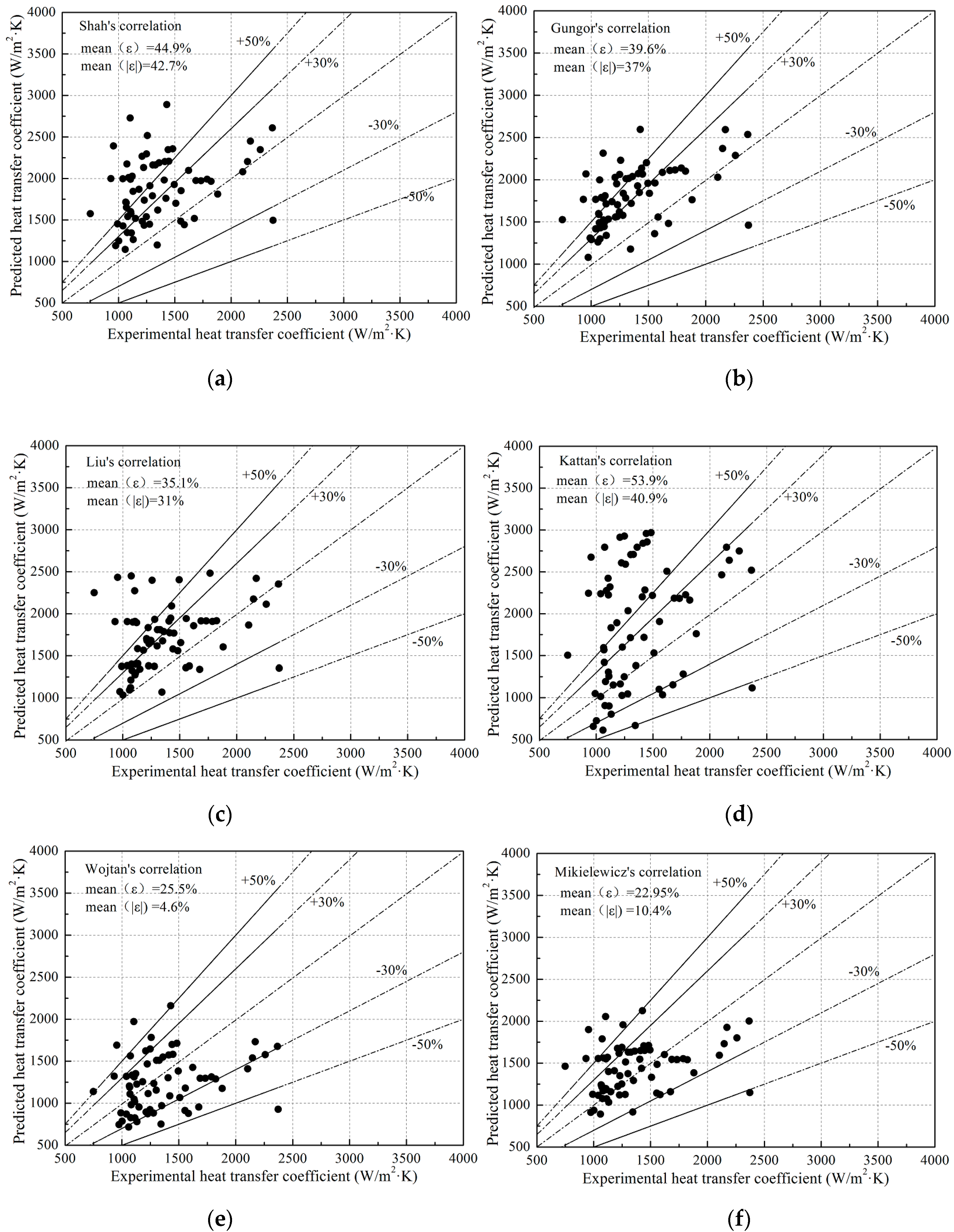
3.1. HTC Correlations in the Two-Phase Continuous Flow

In this section, the experimental HTC data in the two-phase continuous flow were compared to several existing types of correlations, which are listed in Table 3. The mean error and standard deviation of predicted HTC by different correlations were analyzed. The suitable correlation was selected to predict the results in the two-phase continuous flow, which will be one important component of the HTC in the two-phase pulsating flow.

Table 3. Heat transfer coefficient (HTC) correlations in previous literature.

Author	Correlation
Shah [8]	$h_{\mathrm{tp}}/h_{\mathrm{sp}}=MAX({\psi }_{\mathrm{nb}},{\psi }_{\mathrm{cb}})$
	${\psi }_{\mathrm{nb}}=f(Bo) {\psi }_{\mathrm{nb}}=f(Co)$
Gungor [20]	$h_{\mathrm{tp}}=F{h}_l+S{h}_{\mathrm{pool}}$
	$F=1+24000B{o}^{1.16}+1.37{(1/X_{\mathrm{tt}})}^{0.86}$
	$S=\frac{1}{1+1.15\times {10}^{-6}{F}^2{Re}_l{}^{1.17}}$
Liu [22]	$h_{\mathrm{tp}}{}^{}=\sqrt{{(F{h}_l)}^2+{(S{h}_{\mathrm{pool}})}^2}$
	$F={[1+x{Pr}_l(\frac{{\rho }_l}{{\rho }_v}-1)]}^{0.35}$
	$S={(1+0.055F^{0.1}{Re}_l{}^{0.16})}^{-1}$
Kattan [23]	$h_{\mathrm{tp}}=\frac{{\theta }_{\mathrm{dry}}{h}_v+(2\pi -{\theta }_{\mathrm{dry}})h_{\mathrm{wet}}}{2\pi }$
	$h_v=0.023{({Re}_v)}^{0.8}{({Pr}_v)}^{0.4}(k_v/D)$
	$h_{\mathrm{wet}}={[{(h_{\mathrm{cb}})}^3+{(h_{\mathrm{nb}})}^3]}^{1/3}$
	${\theta }_{\mathrm{dry}}={\theta }_{\mathrm{strat}}\frac{(G_{\mathrm{wavy}}-G)}{(G_{\mathrm{wavy}}-G_{\mathrm{strat}})}$
Wojtan [24]	$h_{\mathrm{tp}}=\frac{{\theta }_{\mathrm{dry}}{h}_v+(2\pi -{\theta }_{\mathrm{dry}})h_{\mathrm{wet}}}{2\pi }$
	Slug/Annular/Intermittent zone θdry = 0
	Stratified-wavy zone ${\theta }_{\mathrm{dry}}={\theta }_{\mathrm{strat}}{\left[\frac{(G_{\mathrm{wavy}}-G)}{(G_{\mathrm{wavy}}-G_{\mathrm{strat}})}\right]}^{0.61}$
	Slug-stratified wavy zone ${\theta }_{\mathrm{dry}}={\theta }_{\mathrm{strat}}{\left[\frac{(G_{\mathrm{wavy}}-G)}{(G_{\mathrm{wavy}}-G_{\mathrm{strat}})}\right]}^{0.61}\frac{x}{x_{\mathrm{IA}}}$
Mikielewicz [17]	$\frac{h_{\mathrm{tp}}}{h_l}=\sqrt{R_{MS}^n+\frac{1}{1+P}{(\frac{h_{\mathrm{pool}}}{h_l})}^2}$
	$P=2.53\times {10}^{-3}{Re}^{1.17}B{o}^{0.6}{(R_{MS}-1)}^{-0.65}$
	$R_{MS}=[1+2(\frac{1}{f}-1)xCo{n}^m]\times {(1-x)}^{1/3}+x^3\frac{1}{f_{1z}}$
	$f_{1z}={(\frac{{\mu }_G}{{\mu }_L})}^{0.4}{(\frac{C{p}_L}{C{p}_G})}^{0.4}{(\frac{{\lambda }_L}{{\lambda }_G})}^{0.6}$
	For Laminar flow, n = 2 $f_1=({\rho }_G/{\rho }_L)({\mu }_L/{\mu }_G)$
	For turbulent flow, n = 0.9 $f_1=({\rho }_G/{\rho }_L){({\mu }_L/{\mu }_G)}^{0.25}$
	For conventional channels, m = 0
	For small-diameter channels and mini channels, m = −1

Figure 4 presents the comparisons of the experimental HTC data in the two-phase continuous flow to the different types of existing empirical correlations. It can be seen that the correlations proposed by Shah, Gungor, Liu, and Kattan tended to overpredict the experimental results with mean errors of 42.7%, 37%, 31%, and 40.9%, respectively. Only about 50% of the data fell inside ±30% error window for these four correlations. The dispersion occurred mainly in the higher inlet vapor quality region with a narrower vapor quality range (mainly intermittent and annular flow pattern regions). Compared with the four correlations above, the correlations developed by Wojtan and Mikielewicz had higher accuracy to predict the experimental data with small mean errors of −4.6% and 10.4%. These two correlations predicted 86.7% and 79.4% of the data inside ±30% error windows, respectively.

Figure 4. Comparison of the experimental HTC data and predicted results by empirical HTC correlations: (a) Shah, (b) Gungor, (c) Liu, (d) Kattan, (e) Wojtan, and (f) Mikielewicz.

The summary of all the statistical analysis from the comparisons between experimental data and predicted values is given in Table 4. Although the mean absolute error in Wojtan’s model was larger than that in Mikielewicz’s correlation, Wojtan’s model had the most data points inside an error window of ±30% and ±50%. Therefore, the Wojtan’s model was selected to predict HTC in the R134a two-phase continuous flow.

Table 4. Summary of the statistical analysis of the different correlations.

Correlation	Mean Error (%)	Abs. Mean Error (%)	Standard Deviation (%)	Points Inside an Error Window of
				±30 (%)	±50 (%)
Shah	42.7	44.9	37.9	47	62
Gungor	37.0	39.6	29.1	45.5	73.5
Liu	31.0	35.2	40.1	55.8	82.4
Kattan	40.9	53.9	57.2	51.5	61.8
Wojtan	−4.6	25.5	29.6	86.7	94.1
Mikielewicz	10.5	22.9	29.9	79.4	91.2

$\mathrm{Error}{\epsilon }_i=(h_{pred,i}-h_{exp,i})/h_{exp,i}$; $\mathrm{Mean} \mathrm{error}(\epsilon )=\frac{1}{n}{\displaystyle {\sum }_{i=1}^n{\epsilon }_i}$; $\mathrm{Mean} \mathrm{absolute} \mathrm{error}(\left|\epsilon \right|)=\frac{1}{n}{\displaystyle {\sum }_{i=1}^n\left|{\epsilon }_i\right|}$; $\mathrm{Standard} \mathrm{deviation} (\sigma )=\sqrt{\frac{1}{n}{\displaystyle {\sum }_{i=1}^n{({\epsilon }_i-\epsilon )}^2}}$.

3.2. Model of the HTC Ratio for Two-Phase Pulsating Flow Using RSM

3.2.1. Description about RSM

The RSM, firstly proposed by Box and Wilson [30], is a method to accurately predict the input–response relationships by fully considering the parameter interaction in engineering systems [31,32,33]. It has been popularized in many fields for the design, development, and promotion of new products, as well as in the optimization of existing product designs. With the aid of limited experimental designs, RSM can achieve the regression model of parameters and responses, and intuitively show the correlation curve between parameters and responses using the contour plot and response surface. Therefore, the RSM is used to rearrange the experimental design and further develop the correlation of HTC ratio in the two-phase pulsating flow.

Usually, a second-order model in RSM can be written as follows:

$$y={\beta }_0+{\displaystyle \sum _{i=1}^n{\beta }_i{x}_i}+{\displaystyle \sum _{i=1}^{n-1}{\displaystyle \sum _{j=i+1}^n{\beta }_{ij}}}{x}_i{x}_j+{\displaystyle \sum _{i=1}^n{\beta }_{ii}{x}_i^2}+\epsilon$$

(8)

where y is the response, x_i and x_j represent independent variables; n is the number of variables; β₀, β_i, β_ii, and β_ij (i = 0, 1, 2, …, n; j = 0, 1, 2, …, n) are coefficients for the intercept, linear, quadratic, and interaction terms in the regression model respectively; and ε is the statistical error.

The generic form of HTC correlation is usually written as follows:

$$h=C·x_1{}^{a_1}{x}_2{}^{a_2}·\dots ·x_n{}^{a_n}$$

(9)

where x₁, x₂, …, x_n are general variables closed to HTC. a₁, a₂, and a_n are the power of the number. Additionally, C is the constant term and n is the number of variables. Taking the logarithm of both sides in Equation (9), one can get

$$\ln h=\ln C+{\displaystyle \sum _{i=1}^n{a}_i}{x}_i=\ln C+{\displaystyle \sum _{i=1}^{n-1}{a}_i}{x}_i+a_n{x}_n$$

(10)

Neglecting the statistical error and rewriting Equation (8)

$$y={\beta }_0+{\displaystyle \sum _{i=1}^{n-1}({\beta }_i+{\displaystyle \sum _{j=i+1}^n{\beta }_{ij}}{x}_j}+{\beta }_{ii}{x}_i^{})x_i+x_n({\beta }_n+{\beta }_{nn}{x}_n)$$

(11)

In order to declare the reason why the second-order RSM model is used, the comparisons of Equations (10) and (11) are listed in Table 5.

Table 5. The comparisons of Equations (10) and (11).

Variables	Equation (10)	Equation (11)
Constant term	lnC	β0
Coefficients of xi (i = 1, …, n−1)	${\displaystyle \sum _{i=1}^{n-1}{a}_i}$	${\displaystyle \sum _{i=1}^{n-1}({\beta }_n+{\displaystyle \sum _{j=i+1}^n{\beta }_{ij}}{x}_j}+{\beta }_{ii}{x}_i^{})$
Coefficient of xn	an	βn + βnnxn

It can be seen from the Table 5 that Equations (10) and (11) have a similar format, indicating that the RSM is feasible to obtain the HTC correlation.

3.2.2. Rearrangement of Experimental Data

In the two-phase pulsating flow, the pulsation period, mass flux, and vapor quality all have remarkable effects on the heat transfer performance with a strong interaction. In order to facilitate the analysis, a dimensionless variable called the Strouhal number (St), which represents the ratio of the inertial forces due to the instability of the flow to the inertial forces caused by velocity change, is defined as:

$$St=\frac{fD}{u_m}$$

(12)

where

$$u_m=\frac{G}{x{\rho }_v+(1-x){\rho }_l}$$

(13)

The St number considers the effects of both the pulsation period and mass flux comprehensively. Besides this factor, inlet and outlet vapor quality are also chosen as the designing factors because they determine the flow patterns combined with mass flux. The HTC ratio defined as the ratio of HTC in the pulsating flow (h_pulsating) to that in the continuous flow (h_continuous) is selected as the response. It can be written as follows:

$$h*=\frac{h_{pulsating}}{h_{continuous}}$$

(14)

In this paper, the number of variables is 3, that is, n = 3. x₁, x₂, and x₃ represents the St number, inlet vapor quality x_in, and outlet vapor quality x_out. The experimental variables and varying ranges are given in Table 6. First the factors and varying ranges are the input and the experimental matrix is generated by the RMS design. Then taking the logarithm of both variables and responses, the experimental matrix can be regenerated. Eventually, taking exponentials for both sides of the RSM regression model, the HTC ratio correlation was achieved.

Table 6. Experimental variables and ranges.

Variables	Ranges
St	0.0007	0.0287
xin	0.1	0.4
xout	0.6	0.9

According to the design by RSM, 160 of 264 experimental data were selected to obtain the HTC ratio. The experimental designing parameters and obtained HTC ratio were taken as the Napierian logarithm, and input for the matrix designing by RSM. The RSM design matrix in the form of the Napierian logarithm is shown in Table 6. The factors were tabulated in the middle three columns and the response (the ratio h*) was given in the far right column of Table A1, please see the Appendix A.

3.2.3. Analysis of Variance (ANOVA)

An ANOVA was performed to observe the significance of the model and designing parameters statistically. Table 7 shows the ANOVA results of the regression model for ln(h*). In ANOVA, the sum of squares was adopted to assess the square of deviation from the grand mean. Dividing the sum of squares by the degrees of freedom, one can obtain the mean squares. The F value was calculated using the ratio of the mean square for each term to the mean square for the residual. The value of F was greater than the F-table value or the p-value was less than 0.05, indicating that the model was significant or the corresponding variables had significant influences on the responses.

Table 7. ANOVA table for ln(h*).

Source	Sum of Squares	df	Mean Square	F Value	p-Value Prob > F	Significance
Model	0.8193	9	0.0910	47.71	<0.0001	*
ln(St)	0.2087	1	0.2087	109.38	<0.0001	*
ln(xin)	0.0100	1	0.0100	5.25	0.0233	*
ln(xout)	0.1072	1	0.1072	56.21	<0.0001	*
ln(St) ln(xin)	0.0029	1	0.0029	1.51	0.2215
ln(St) ln(xout)	0.0067	1	0.0067	3.52	0.0625
ln(xin) ln(xout)	0.0586	1	0.0586	30.70	<0.0001	*
(ln(St))2	0.0583	1	0.0583	30.56	<0.0001	*
(ln(xin))2	0.0753	1	0.0753	39.49	<0.0001	*
(ln(xout)) 2	0.0028	1	0.0028	1.48	0.2250
Residual	0.2862	150	0.0019
Lack of Fit	0.2300	121	0.0019	0.98	0.5503
Pure Error	0.0562	29	0.0019
Cor Total	1.1054	159
Adeq Precision			34.433

* represents this term have significant effect.

As Table 7 shows, the main effects of ln(St), ln(x_in), and ln(x_out), as well as the interaction terms of ln(St) and ln(x_in) and ln(x_in) and ln(x_out) and the quadratic terms of (ln(St))² and (ln(x_in))² were statistically significant because their p-values were smaller than 0.05. “Adeq Precision” measures the signal to noise ratio. An “Adeq Precision” greater than 4 is desirable. The ratio of 34.433 indicates an adequate signal. Therefore, this model can be used to predict the results.

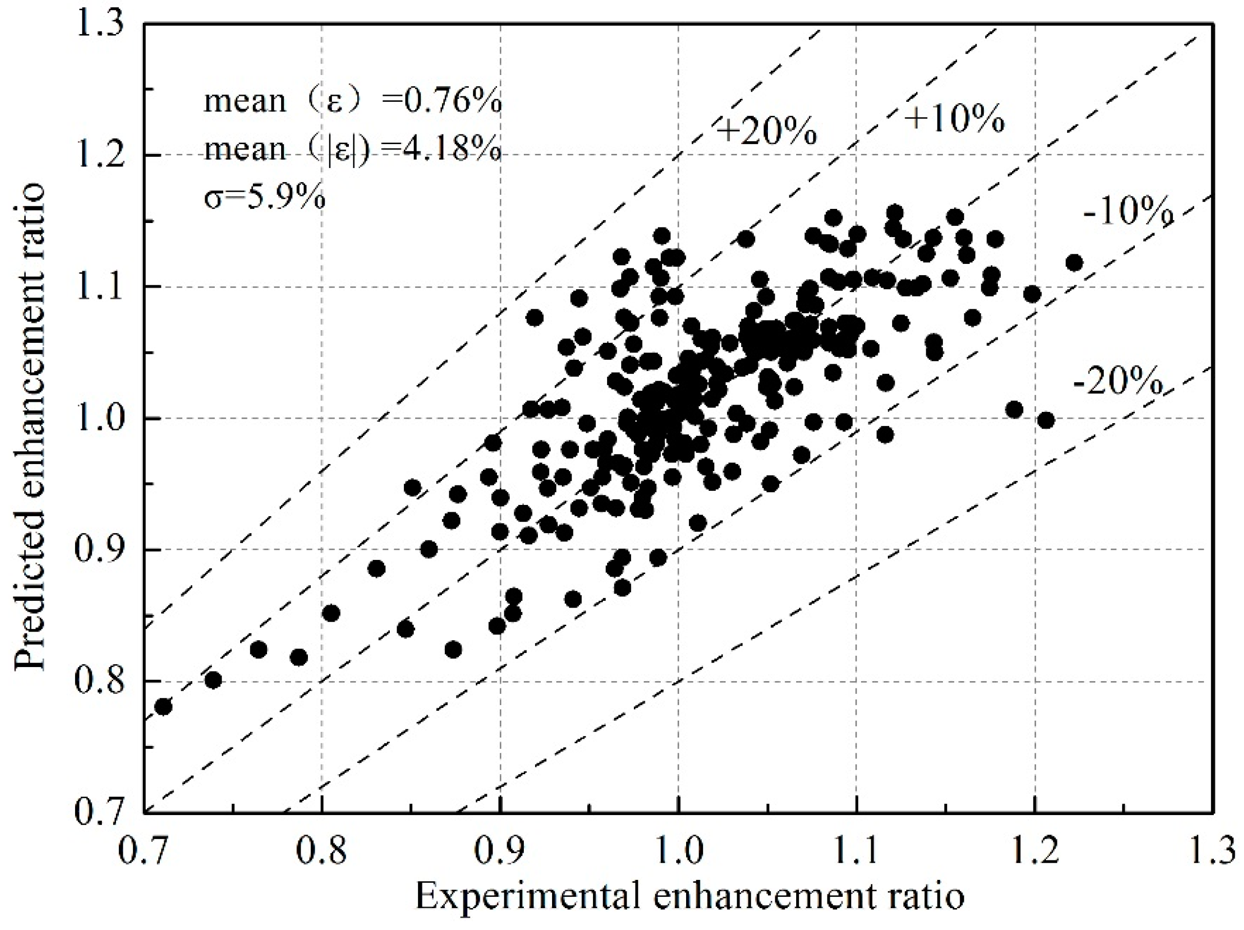
3.2.4. RSM Regression Model for the HTC Ratio

After the ANOVA, the regression model developed by RSM is finally given as follows:

$$\begin{array}{l}\ln (h*)=-1.054-0.242\times \ln (St)-0.614\times \ln (x_{\mathrm{in}})-0.498\times \ln (x_{\mathrm{out}})\\ -0.0098\times \ln (St)\times \ln (x_{\mathrm{in}})+0.059\times \ln (St)\times \ln (x_{\mathrm{out}})-0.245\times \ln (x_{\mathrm{in}})\times \ln (x_{\mathrm{out}})\\ -0.027\times \ln (St)^2-0.145\times \ln (x_{\mathrm{in}})^2-0.307\times \ln (x_{\mathrm{out}})^2\end{array}$$

(15)

Taking the exponent for both sides, the Equation (15) can be transformed as:

$$h*=0.348{(St)}^{j1}{(x_{\mathrm{in}})}^{j2}{(x_{\mathrm{out}})}^{j3}$$

(16)

where

$$\begin{gathered} j1=-0.242-0.027ln(St)-0.0098\ln (x_{\mathrm{in}})+0.059\ln (x_{\mathrm{out}}) \\ j2=-0.614-0.145\ln (x_{\mathrm{in}})-0.245\ln (x_{\mathrm{out}}) \\ j3=-0.498-0.307\ln (x_{\mathrm{out}}) \end{gathered}$$

The normal probability plot for the residuals obtained from RSM for the regression model is displayed in Figure 5. It can be seen that all the residuals generally fell on or near the diagonal line, indicating that the errors satisfied normal distribution. In addition, almost all internally studentized residuals were close to zero, indicating that the regression model of the response had a better prediction precision.

Figure 5. Normal probability plot of residuals for the regression model.

Figure 6 presents the comparisons between RSM predicted results and 246 experimental data of the HTC ratio. It can be seen that the RSM model tended to predict the experimental data accurately with a mean error of 0.76% and a standard deviation of 5.9%. Of the data 91.4% was contained inside a ± 10% error window while 100% of the data lay in a ±20% error window, indicating that the prediction of the RSM model of HTC ratio was satisfactory. Next, the RSM model of the HTC ratio and Wojtan’s model in the continuous flow were combined to develop a model to predict the HTC in the two-phase pulsating flow.

Figure 6. Response surface methodology (RSM) prediction vs. experimental data for HTC ratio in the two phase pulsating flow.

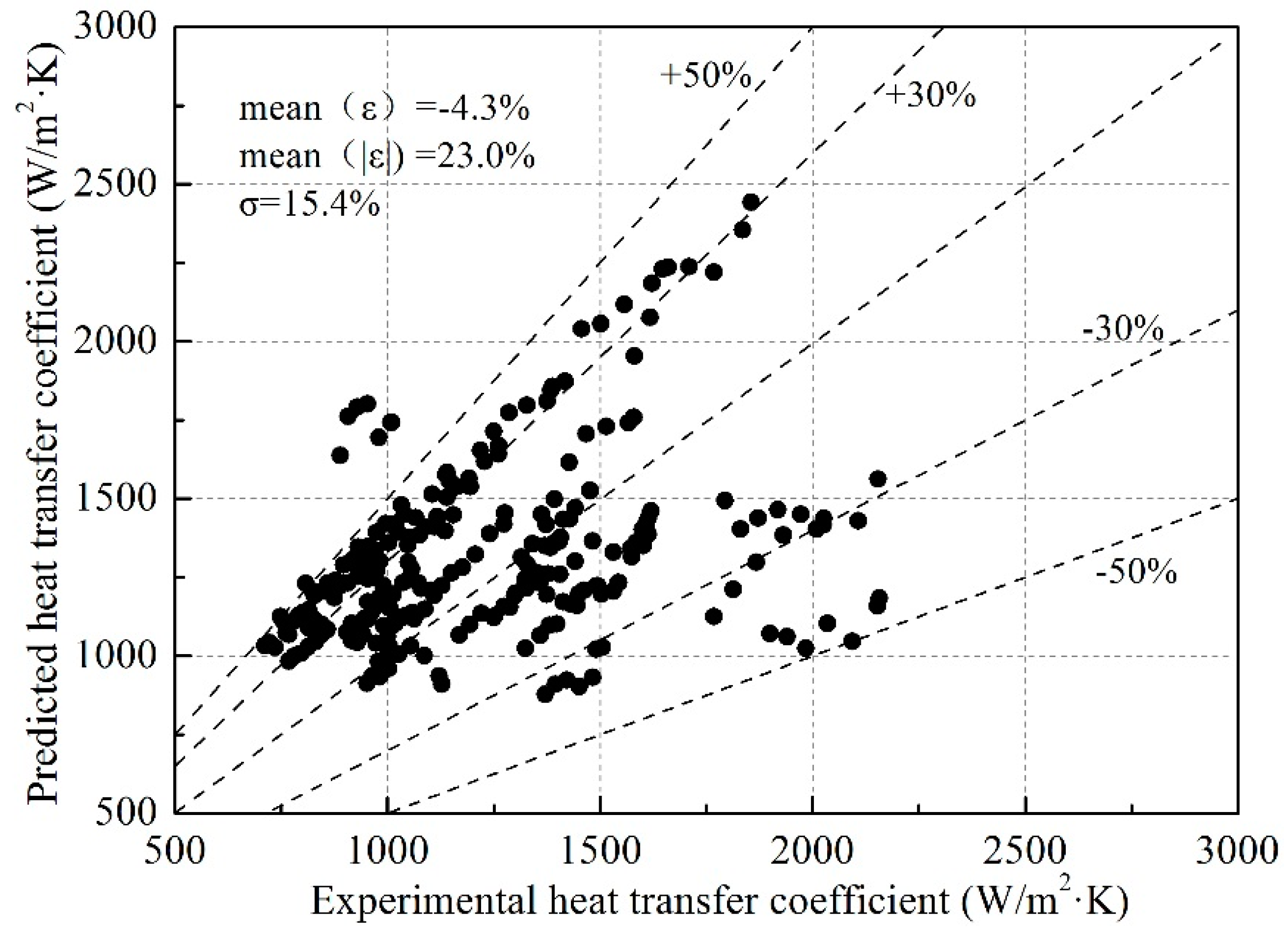
3.3. HTC model for R134a Two-Phase Pulsating Flow Boiling

The heat transfer characteristic in the R134a two-phase pulsating flow is much more complicated compared with the two-phase continuous flow. It can be affected by many parameters, such as the pulsation period, mass flow rate, vapor quality, and so on. After obtaining the HTC ratio model by RSM, the final prediction of HTC in the two-phase pulsating flow can be written as Wojtan’s model multiplying by the RSM model (Equation (16)).

The comparison between the correlation predicted and experimental HTC in the two-phase pulsating flow is depicted in Figure 7. The results obtained with the new model shows a low mean error of −4.3% and a low standard deviation of 15.4%. Of the data 81.2% and 95.1% were contained inside the ±30% and ±50% error window, indicating that the correlation could predict the HTC in the two-phase pulsating flow well. It should be noted that a large dispersion between prediction and experimental values occurred at a high mass flow rate with a high inlet vapor quality. The error was mainly due to the overprediction of the annular zone in the two-phase continuous flow, as shown in Figure 4e.

Figure 7. Comparison of the experimental HTC data to the predicted results by the correlation.

4. Conclusions

In this study, a new model for predicting HTC in the R134a liquid–vapor two-phase pulsating flow was developed based on the heat transfer model in the two-phase continuous flow and response surface methodology. The conclusions can be summarized as follows:

(1)

Six existing models for heat transfer in the two-phase continuous flow were compared with our experimental data. Results show that the Wojtan’s model had the smallest mean error and the most data lying in the ±50% error window. Therefore, the Wojtan’s model was selected as a basis for predicting HTC in the R134a two-phase continuous flow.

(2)

RSM was carried out to rearrange the experimental data to obtain the regression model for the HTC ratio. ANOVA was performed to test the statistical significance of the model. The small error between RSM predicted data and experimental results shows that the model was satisfactory.

(3)

A new model for HTC in the R134a two-phase pulsating flow was finally obtained by multiplying the Wojtan’s model in continuous flow with the RSM regression model for the ratio. The new correlation produced a small error of −4.3% and a standard deviation of 15.4% compared with experimental results, indicating that the new model can predict the HTC in the R134a two-phase pulsating flow boiling well.

References

1. Fernández-Seara, J.; Pardiñas, Á.Á.; Diz, R. Heat transfer enhancement of ammonia pool boiling with an integral-fin tube. Int. J. Refrig. 2016, 69, 175–185. [Google Scholar] [CrossRef]
2. Kærn, M.R.; Elmegaard, B.; Meyer, K.E.; Palm, B.; Holst, J. Continuous versus pulsating flow boiling. Experimental comparison, visualization, and statistical analysis. Sci. Technol. Built Environ. 2017, 23, 983–996. [Google Scholar]
3. Li, G.; Zheng, Y.; Hu, G.; Zhang, Z.; Xu, Y. Experimental study of the heat transfer enhancement from a circular cylinder in laminar pulsating cross-flows. Heat Transf. Eng. 2016, 37, 535–544. [Google Scholar] [CrossRef]
4. Bohdal, T.; Kuczyński, W. Investigation of boiling of refrigeration medium under periodic disturbance conditions. Exp. Heat Transf. 2005, 18, 135–151. [Google Scholar] [CrossRef]
5. Chen, C.A.; Chang, W.R.; Lin, T.F. Time periodic flow boiling heat transfer of R-134a and associated bubble characteristics in a narrow annular duct due to flow rate oscillation. Int. J. Heat Mass Transf. 2010, 53, 3593–3606. [Google Scholar] [CrossRef]
6. Roh, C.W.; Kim, M.S. Enhancement of heat pump performance by pulsation of refrigerant flow using a solenoid-driven control valve. Int. J. Refrig. 2012, 35, 1547–1557. [Google Scholar] [CrossRef]
7. Dittus, F.W.; Boelter, L.M. Heat transfer in automobile radiators of the tubular type. Int. Commun. Heat Mass Transf. 2012, 12, 3–22. [Google Scholar] [CrossRef]
8. Shah, M.M. Chart correlation for saturated boiling heat transfer: Equations and further study. ASHRAE Trans. 1982, 88, 185–196. [Google Scholar]
9. Jabardo, J.S.; Bandarra Filho, E.P.; Lima, C.U. New correlation for convective boiling of pure halocarbon refrigerants flowing in horizontal tubes. J. Braz. Soc. Mech. Sci. 1999, 21, 245–258. [Google Scholar]
10. Chaddock, J. Film coefficients for in-tube evaporation of ammonia and R-502 with and without small percentages of mineral oil. Ashrae Trans. 1986, 92, 22–40. [Google Scholar]
11. Wattelet, J.P.; Chato, J.C.; Jabardo, J.M.; Panek, J.S.; Renie, J.P. An experimental comparison of evaporation characteristics of HFC-134a and CFC-12. In Proceedings of the XVIIIth International Congress of Refrigeration, Montreal, QC, Canada, 10–17 August 1991. [Google Scholar]
12. Panek, J.S. Evaporation Heat Transfer and Pressure Drop in Ozone-Safe Refrigerants and Refrigerant-Oil Mixtures; Air Conditioning and Refrigeration Center, College of Engineering, University of Illinois at Urbana-Champaign: Champaign, IL, USA, 1992. [Google Scholar]
13. Tran, T.N.; Wambsganss, M.W.; France, D.M. Small circular-and rectangular-channel boiling with two refrigerants. Int. J. Multiph. Flow 1996, 22, 485–498. [Google Scholar] [CrossRef]
14. Kew, P.A.; Cornwell, K. Correlations for the prediction of boiling heat transfer in small-diameter channels. Appl. Therm. Eng. 1997, 17, 705–715. [Google Scholar] [CrossRef]
15. Lazarek, G.M.; Black, S.H. Evaporative heat transfer, pressure drop and critical heat flux in a small vertical tube with R-113. Int. J. Heat Mass Transf. 1982, 25, 945–960. [Google Scholar] [CrossRef]
16. da Silva Lima, R.J.; Quibén, J.M.; Thome, J.R. Flow boiling in horizontal smooth tubes: New heat transfer results for R-134a at three saturation temperatures. Appl. Therm. Eng. 2009, 29, 1289–1298. [Google Scholar] [CrossRef]
17. Mikielewicz, D. A new method for determination of flow boiling heat transfer coefficient in conventional-diameter channels and minichannels. Heat Transf. Eng. 2010, 31, 276–287. [Google Scholar] [CrossRef]
18. Sardeshpande, M.V.; Ranade, V.V. Two-phase flow boiling in small channels: A brief review. Sadhana 2013, 38, 1083–1126. [Google Scholar] [CrossRef]
19. Cooper, M.G. Saturated Nucleate Pool Boiling-A Simple Correlation. IChemE Symp. Ser. 1984, 86, 786. [Google Scholar]
20. Gungor, K.E.; Winterton, R.H. A general correlation for flow boiling in tubes and annuli. Int. J. Heat Mass Transf. 1986, 29, 351–358. [Google Scholar] [CrossRef]
21. Gungor, K.E.; Winterton, R.H.S. Simplified general correlation for saturated flow boiling and comparisons of correlations with data. Chem. Eng. Res. Des. 1987, 65, 148–156. [Google Scholar]
22. Liu, Z.; Winterton, R.H.S. A general correlation for saturated and subcooled flow boiling in tubes and annuli, based on a nucleate pool boiling equation. Int. J. Heat Mass Transf. 1991, 34, 2759–2766. [Google Scholar] [CrossRef]
23. Kattan, N.; Thome, J.R.; Favrat, D. Flow boiling in horizontal tubes: Part 3—Development of a new heat transfer model based on flow pattern. J. Heat Transf. 1998, 120, 156–165. [Google Scholar] [CrossRef]
24. Wojtan, L.; Ursenbacher, T.; Thome, J.R. Investigation of flow boiling in horizontal tubes: Part II—Development of a new heat transfer model for stratified-wavy, dryout and mist flow regimes. Int. J. Heat Mass Transf. 2005, 48, 2970–2985. [Google Scholar] [CrossRef]
25. Wang, X.; Tang, K.; Hrnjak, P.S. Evaporator performance enhancement by pulsation width modulation (PWM). Appl. Therm. Eng. 2016, 99, 825–833. [Google Scholar] [CrossRef]
26. Yang, P.; Zhang, Y.; Wang, X.; Liu, Y.W. Heat transfer measurement and flow regime visualization of two-phase pulsating flow in an evaporator. Int. J. Heat Mass Transf. 2018, 127, 1014–1024. [Google Scholar] [CrossRef]
27. ASME. Measurement of Fluid Flow in Pipes Using Orifice, Nozzle, and Venture; Standard MFC-3M-2004; American Society of Mechanical Engineers: New York, NY, USA, 2004. [Google Scholar]
28. ASME. Flow Measurement; ANSI/ASME Standard PTC 19.5–2004 (RA13); American Society of Mechanical Engineers: New York, NY, USA, 2013. [Google Scholar]
29. Kim, N.H.; Youn, B.; Webb, R.L. Air-side heat transfer and friction correlations for plain fin-and-tube heat exchangers with staggered tube arrangements. J. Heat Transf. 1999, 121, 662–667. [Google Scholar] [CrossRef]
30. Box, G.E.; Wilson, K.B. On the experimental attainment of optimum conditions. J. R. Stat. Soc. Ser. B (Methodol.) 1951, 13, 1–38. [Google Scholar] [CrossRef]
31. Yang, P.; Liu, Y.W.; Zhong, G.Y. Prediction and parametric analysis of acoustic streaming in a thermoacoustic Stirling heat engine with a jet pump using response surface methodology. Appl. Therm. Eng. 2016, 103, 1004–1013. [Google Scholar] [CrossRef]
32. Liu, Y.; Liu, L.; Liang, L.; Liu, X.; Li, J. Thermodynamic optimization of the recuperative heat exchanger for Joule–Thomson cryocoolers using response surface methodology. Int. J. Refrig. 2015, 60, 155–165. [Google Scholar] [CrossRef]
33. Hariharan, N.M.; Sivashanmugam, P.; Kasthurirengan, S. Optimization of thermoacoustic primemover using response surface methodology. HVAC R Res. 2012, 18, 890–903. [Google Scholar]