Article

Optimal Design of a Combined Cooling, Heating, and Power System and Its Ability to Adapt to Uncertainty

1
Key Laboratory of Energy Thermal Conversion and Control of Ministry of Education, School of Energy and Environment, Southeast University, Nanjing 210096, China
2
Department of Electrical and Computer Engineering, Technical University of Munich, 85748 Munich, Germany
3
Yunnan Electric Power Research Institute, CSG, Kunming 650228, China
*
Author to whom correspondence should be addressed.
Energies 2020, 13(14), 3588; https://doi.org/10.3390/en13143588
Submission received: 8 June 2020 / Revised: 3 July 2020 / Accepted: 7 July 2020 / Published: 11 July 2020
(This article belongs to the Section G: Energy and Buildings)

Abstract

:
To realize the best performances of the distributed energy system (DES), many uncertainties including demands, solar radiation, natural gas, and electricity prices must be addressed properly in the planning process. This study aims to study the optimal sizing and performances of a hybrid combined cooling, heating, and power (CCHP) system under uncertainty in consideration of the operation parameters, including the lowest electric load ratio (LELR) and the electric cooling ratio (ECR). In addition, the ability of the system to adapt to uncertainty is analyzed. The above works are implemented separately under three operation strategies with multi-objectives in energy and cost saving, as well as CO2 reducing. Results show that the system with optimized operation parameters performs better in both the deterministic and uncertain conditions. When the ECRs in the summer and in mid-season as well as the LELR are set at 50.00%, 50.00%, and 20.00% respectively, the system operating in the strategy of following the electric load has the best ability to adapt to uncertainty. In addition, among all the uncertainties, the single uncertain natural gas price and the single uncertain heating demand have the smallest and largest effects on the optimal design respectively.

1. Introduction

In recent years, the energy system is on its way to be transformed to meet the requirements of energy saving and environment protection. In this way, many distributed energy systems (DESs) including the CHP (combined heating and power) system, the CCHP (combined cooling heating and power) system, and other hybrid systems can be planned for commercial buildings, residential districts, and industry parks because of their efficient, economic, and environmental performances. At the design stage of a DES for a building, some parameters, such as the estimated energy demands, natural resources, and energy prices, are regarded as the fixed values. Nevertheless, at the operation stage in the real application, all these parameters fluctuate with different uncertain characteristics, which can cause a worse performance than the expected one. Therefore, the uncertainty must be handled in both the planning and operation [1].
Many authors have implemented works on tackling the uncertainty in DES planning with different methods, including fuzzy programming [2], robust optimization [3], and stochastic programming [4]. In the fuzzy approach, Moradi et al. [5] used fuzzy programming to deal with the uncertain electrical and thermal demands as well as the natural gas and electrical power prices in a CHP system. Considering the uncertainty in load demand and fuel cost, Mavrotas et al. [6,7] proposed a fuzzy mathematical framework to plan an energy system. Zhou et al. [8] employed a fuzzy interval possibilistic model to handle the CO2 emission factor uncertainty in a sustainable electrical power system. Lu et al. [9] addressed the uncertainties of energy price and CO2 emission factors in the energy system with an interval-fuzzy possibilistic programming model. Based on a life cycle assessment, Li et al. [10] employed a fuzzy rough set to deal with the uncertainties existing in natural resources to evaluate the environmental impact for a distributed renewable energy system. In the robust approach, Majewski et al. [11] addressed the uncertain data of energy demands and the prices in a CCHP system based on a proposed robust model. Luo et al. [12] carried out robust design work for a CCHP system accounting for uncertain demands and photovoltaic output power. Niu et al. [13] planned a renewable cooling resource in a robust way considering demands and renewable energy uncertainties. Based on the minimax regret criterion, Yokoyama et al. [14] carried out robust optimal design works for a gas turbine co-generation system in consideration of uncertain energy demands. Roberts et al. [15] carried out a robust sizing for an energy system in a probabilistic scenario-based way, accounting for uncertain demands and natural resources. In the stochastic approach, Mavromatidis et al. [16] employed the stochastic model in planning for a distributed energy system while considering uncertain energy prices, emission factors, demands, and solar radiation. Incorporating long term uncertainties of loads and prices, Onishi et al. [17] used a stochastic model to get the optimal design for a tri-generation system. Afzali et al. [18] employed a stochastic method to deal with uncertain demands and energy prices when planning an energy system for an urban community. Yang et al. [19] accounted for uncertainties of demands, solar radiation, wind speed, and energy prices in the planning work for CCHP systems. Vaderobli et al. [20] addressed the uncertainties of weather and cost in a renewable energy system with stochastic optimization.
Most of the above works presented for a CHP or CCHP system focus only on the optimal sizing under uncertainty while ignoring the optimization of operation parameters, such as the lowest electric load ratio and the electric cooling ratio. In the deterministic optimization for a CCHP system [21], the operation parameters have apparent effects on the system performance and design. In uncertain optimization, however, it needs further research about how these operation parameters influence the optimal design for a CCHP or CHP system and the ability of the system to adapt to uncertainty. Based on these, the works in this study mainly lie in the following aspects: (1) the effects of multi-uncertainties on a CCHP system planning is researched; (2) the effects of operation parameters on the ability of the system to adapt to uncertainty is investigated; and (3) the effects of a single uncertainty in generated scenarios on system planning is analyzed. This study is composed of six sections. Section 2 presents a system description about the system structure, the operation strategies, and system performances. Section 3 shows the optimization under uncertainty, including the stochastic programming method, the proposed model, and algorithm. Section 4 provides the information about the hotel and case set. Section 5 implements the results from the analysis, and Section 6 concludes the paper.

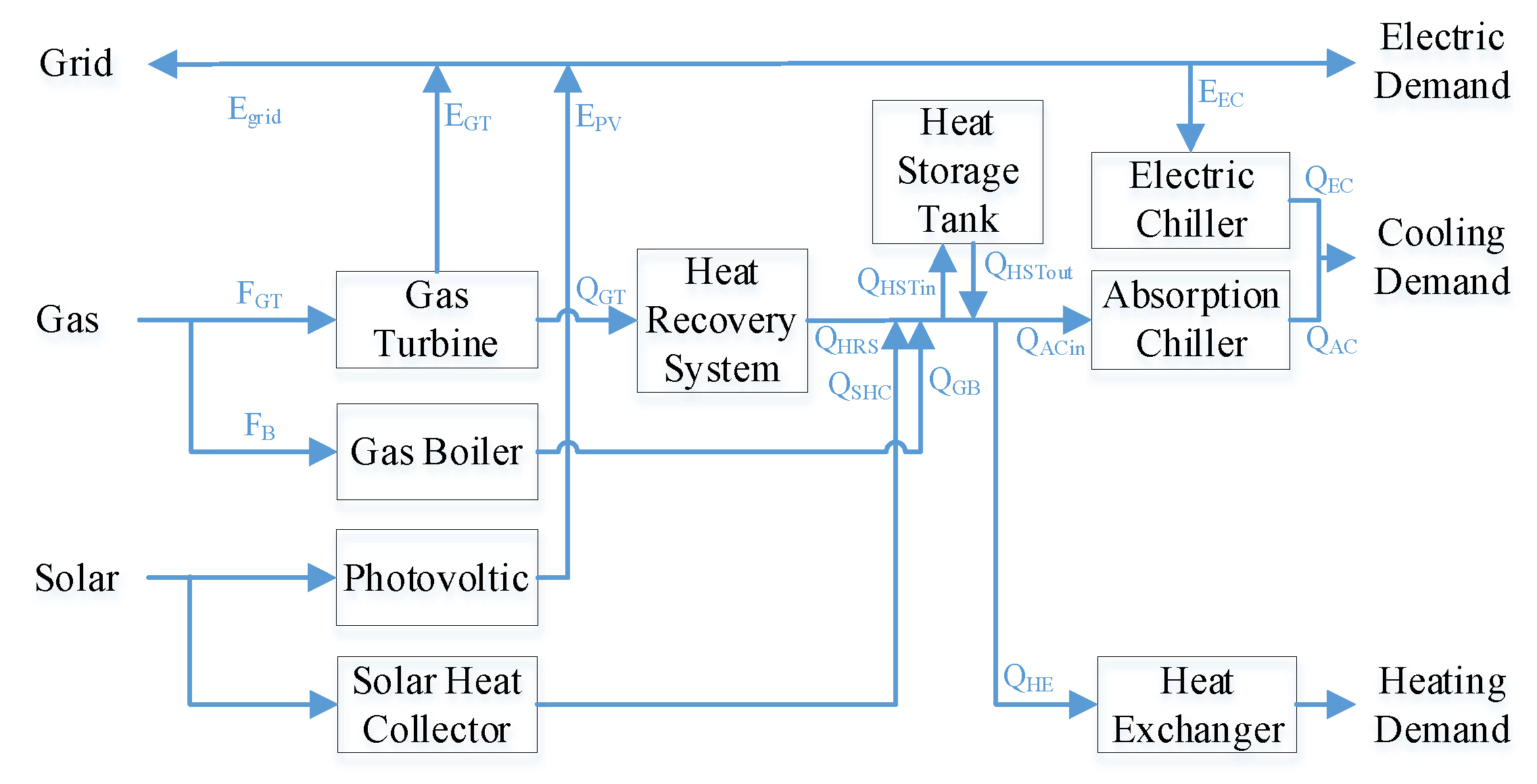
2. System Description

2.1. System Configuration

The planned hybrid CCHP system in this study is shown in Figure 1. The technical and economic parameters can be found in Appendix A.1. In the system, the energy balances are as follows:
(1)
Cooling energy balance:
Q C = Q E C + Q A C
(2)
Heating energy balance:
Q H = ( Q H R S + Q G B + Q S H C Q H S T i n + Q H S T o u t Q A C i n ) η H E
(3)
Electric energy balance:
E = E G T + E P V + E g r i d E E C

2.2. Operation Strategy

Following the thermal load (FTL) [22], following the electric load (FEL) [23], and following the hybrid electric-thermal load (FHL) [24] are the three basic operating strategies for a CCHP system. When the CCHP system operates in FTL, the gas turbine (GT) gives priority to meet the heating demand. When the system operates in FEL, the gas turbine (GT) gives priority to meet the electric demand. In both of these two strategies, the unmet heating and electric demands are covered by a gas boiler (GB) and a state grid, respectively. When the system operates in FHL, if the heat-to-electric ratio of the GT is in part B of Figure 2, the system operates in FEL, or else it operates in FHL. The specific logic of the strategies is defined in Appendix A.2.

2.3. System Performance

The integrated performance (IP), which is composed of the annual total cost saving (ATCS), the primary energy saving (PES), and the carbon dioxide emission reduction (CDER), is used as an objective in the presented study, which is expressed by [25,26]:
I P = ω 1 A T C S + ω 2 P E S + ω 3 C O 2 E R ,
where ATCS, PES, and CO2ER are denoted by f 1 , f 2 , and f 3 respectively, and then the integrated performance is described as:
I P = ω 1 f 1 + ω 2 f 2 + ω 3 f 3 ,
where ω i = 1 3 ( i = 1 , 2 , 3 ) are the weights of each criterion. The specific formulations of ATCS, PES, and CDER are shown in Appendix A.3.

3. Optimization under Uncertainty

3.1. Two-Stage Stochastic Programming

The two-stage stochastic programming problem [4] is used to handle the uncertainty in the planning process. Its basic mathematical model is shown as follows:
Stage 1:
min x X { g ( x ) : = c T x + E [ Q ( x , ξ ) ] } ,
Stage 2:
min y q T y , s . t . T x + W y h ,
where x R n is the decision variable or the here-and-now variable in the first stage, while y R n is the process variable or the wait-and-see variable in the second stage, and ξ = ( q ,   T ,   W ,   h ) denotes the uncertain factors in the second stage.
After sampling, the above problem can be solved. Monte Carlo sampling is one of the sampling techniques used to simulate the future situation of uncertain factors. Based on the given probability distribution, N samples of uncertainty are generated, which is ξ = ( ξ 1 , ξ 2 , , ξ n ) . Combining with the sample average approximation (SAA) method, the expectation function q ( x ) = E [ Q ( x , ξ ) ] in Equation (1) transforms into:
q ¯ N ( x ) = 1 N j = 1 N Q ( x , ξ j ) ,
which then turns the two-stage problem into:
min x X { g ( x ) : = c T x + 1 N j = 1 N Q ( x , ξ j ) } .

3.2. Stochastic Programming Model for the CCHP System

To divide the optimization problem into two stages, the integrated performance is transformed as follows:
I P = ω 1 f 1 + ω 2 f 2 + ω 3 f 3 = ω 1 ( 1 + C f 11 + C f 12 ) + ω 2 f 2 + ω 3 f 3 ,
where C is the constant, while f 11 and f 12 are the investment cost and operation cost of the CCHP system, respectively.
According to the transformed integrated performance and the basic process of optimization, the two-stage stochastic programming model is created as follows:
Stage 1:
max d 1 3 { 1 + C f 11 ( d ) + E [ C f 12 ( d , ξ ) + f 2 ( d , ξ ) + f 3 ( d , ξ ) ] } , s . t . φ d ( d ) = 0 , ψ d ( d ) 0 ,
Stage 2:
max o [ f 12 ( d , ξ , o ) + f 2 ( d , ξ , o ) + f 3 ( d , ξ , o ) ] , s . t . φ o ( d , ξ , o ) = 0 , ψ o ( d , ξ , o ) 0 .
where d is the design variable, including the optimal capacity of each equipment and operation parameters; o is the operation variable, including the gas consumption and electricity consumption; ξ is the uncertainty, including uncertain demands, energies prices, and solar radiation; φ d and ψ d are equality and inequality constraints for the design variables, respectively; and φ o and ψ o are the equality and inequality constraints for the operation variables, respectively. In addition, the uncertainties of demands, solar radiation, and the natural gas and grid electricity prices are addressed in the model; their probability distributions are shown in Appendix A.4.

3.3. Optimization Algorithm

To solve the nonlinear problem, the artificial bee colony (ABC) algorithm [27] is employed in this study. The basic process to realize stochastic programming optimization by the ABC is depicted in Figure 3 while the process of the ABC is presented in Algorithm 1.
Algorithm 1: ABC algorithm optimization process.
Input: Economic and technical parameters, scenarios of demands, solar radiation, and energy prices
   Step 1: Generate all food sources and variables randomly.
   Step 2: Evaluate the fitness of all foods according to the fitness function, given by Equation (4).
Repeat
   Step 3: Employ bee search:
   Compute the objectives of all scenarios and update the food source according to the best IP.
   Step 4: Onlooker bee search:
   Compute the objectives of all scenarios and update the food source according to the best IP.
   Step 5: If trail number > limit, then go to step 6. Otherwise, go to step 7.
   Step 6: Scout bee search:
   Generate a new food source and replace the old one if the new one is better.
   Step 7: Record the best food source.
Until: Max iteration > ε
Output: Optimal capacities, LELRs, and ECRs

4. Case Study

4.1. Hotel Description

The U.S. Department of Energy [28] simulated demands for different types of buildings, which include hotels, schools, and hospitals. In this study, a large hotel that is located at Ohio State University (shown in Figure 4) is used to implement the study. The local climate is a temperate continental climate. July is on average the warmest month, the average high and low temperatures of which are 30.0 and 17.8 °C, respectively; January is on average the coolest month, the average high and low temperatures of which are 2.8 and −7.2 °C, respectively [29]. Some information about the hotel is shown in Table 1. Figure 5a,b shows the demands and solar radiation, respectively. The U.S. Energy Information Administration [30,31] provides the natural gas and grid electricity prices, which are 5.99 dollars per thousand cubic feet and 9.94 cents per kilowatt hour, respectively.

4.2. Simulation Cases

To investigate the effects of electric cooling ratios in the summer (ECR_S) and in mid-season (ECR_M) as well as the lowest electric load ratio (LELR) on system planning, several cases were set in this paper, which are depicted in Table 2. Cases 1–3 were implemented under the deterministic condition, in which the operation parameters are given as 50%, 50%, and 20% [32] respectively in case 1; only the ECRs were optimized in case 2, while the two kinds of parameters were optimized in case 3. Cases 4–6 were carried out under an uncertain condition; the results of the cases were then compared to that of case 1 to study the effect of operation parameters on the ability of the system to adapt uncertainty. In addition, the parameters of the ABC algorithm of cases 1–6 are presented in Appendix A.5.

5. Results and Analysis

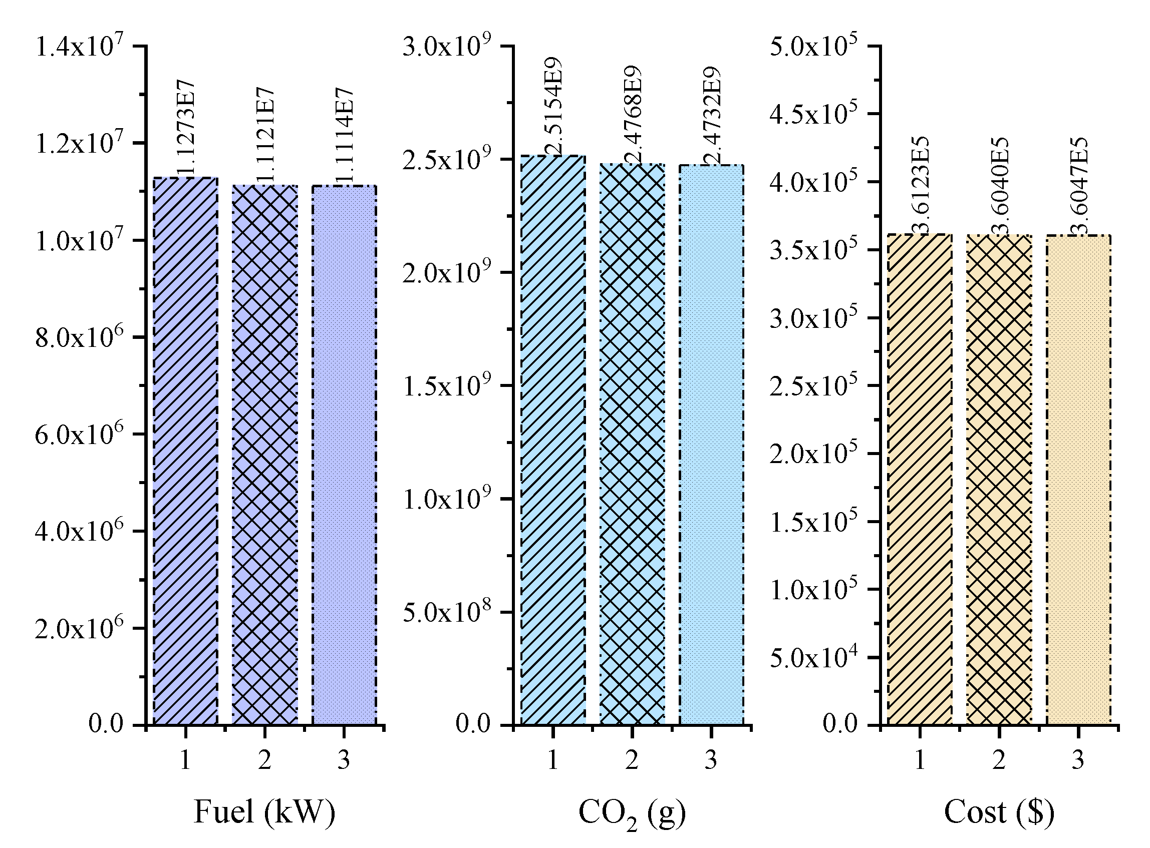
5.1. Result of Deterministic Conditions

Table 3 and Table 4 show the system performances and the optimal design of cases 1–3, respectively. It can be seen from Table 3 that following the electric load (FEL) is the best operation strategy for cases 1–3, and the integrated performance (IP) is 36.00%, 36.63%, and 36.67% respectively. In addition, case 3 performs best among the three strategies on the whole with 33.29% of PES, 47.62% of CDER, and 29.10% of ATCS because the optimal lowest electric load ratio (LELR) and the electric cooling ratios in the summer (ECR_S) and in mid-season (ECR_M) are optimized. Table 4 shows that the LELR, ECR_S, and ECR_M of case 3 in FEL are 5.75%, 37.74%, and 60.38% respectively. Figure 6 presents the annual fuel consumption, the CO2 emission, and the cost of cases 1–3 when the system operates in the best operation strategy (FEL); it can be seen that the annual values of case 3 are 1.1114 × 10⁷ kW, 2.4732 × 10⁹ g, and 3.6047 × 10⁵ dollars, respectively.

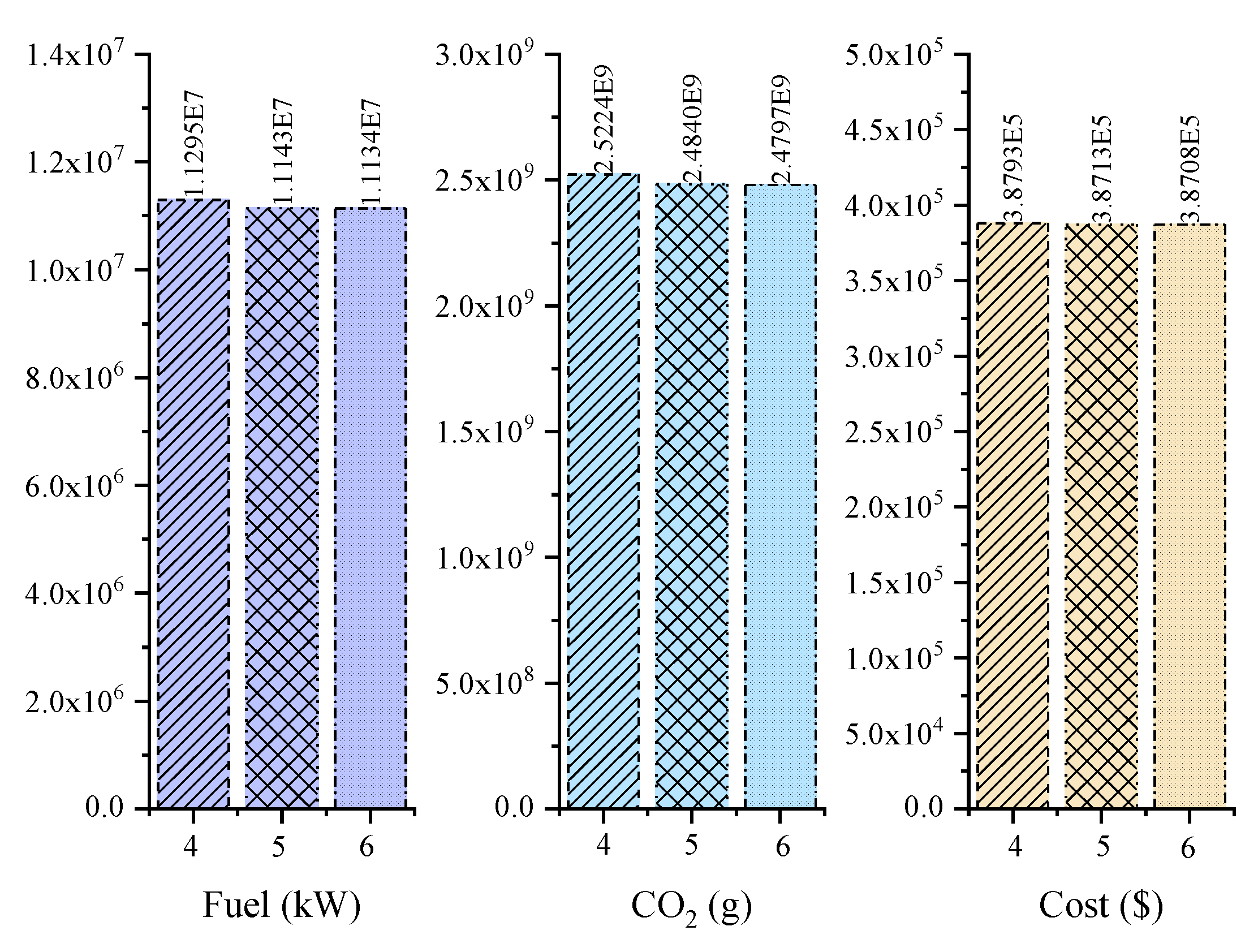
5.2. Result of Uncertain Conditions

5.2.1. Effect of Multi-Uncertainties to System Planning

Uncertainties of demands, solar radiation, and energy prices are handled in cases 4–6, the system performances of which are shown in Table 5. It can be seen that the performances of uncertain cases 4–6 are similar to those of deterministic cases 1–3. Case 6 with optimized LELR and ECRs in FEL are best while 33.17% of the primary energy, 47.48% of CO2, and 31.24% of the total cost are reduced annually. To be specific, Figure 7 depicts that the system operating in the best operation strategy (FEL) of case 6 consumes 1.1134 × 10⁷ kW natural gas, generates 2.4797 × 10⁹ g CO2, and costs 3.8708 × 10⁵ dollars annually, and all the values are the lowest among the three uncertain cases.
Table 6 presents the optimal design of uncertain cases 4–6. To analyze the ability of the system to adapt to uncertainty, the results of the uncertain cases 4–6 and the deterministic cases 1–3 are compared; the cascade color table is shown in Table 7, which is based on the absolute deviation of the cases. It can be seen that on the whole, case 4 performs best to handle uncertainty with the lowest fluctuation of optimal design while the capacities of case 6 deviates from case 3 most significantly among the three uncertain cases.

5.2.2. Effect of a Single Uncertainty to System Planning

The previous section shows that the ability of case 6 in tackling multi-uncertainties is the worst among the uncertain cases, but it has the best performances in efficient, environmental, and economic factors when the system operates in FEL. Therefore, this part analyzes the effect of a single uncertainty of case 6 in relation to the system planning in FEL.
Table 8 depicts the optimal design while Table 9 shows the optimal operation and cost under the different single uncertainties of case 6. It can be seen from Table 8 that the case under the single uncertain natural gas price has the largest LELR (6.34%), while all the other single uncertainties make the lowest electric load ratio decline into around 2.00%.
To study the degree of effects of every single uncertainty on system planning, the color cascade tables are created, as shown in Table 10 and Table 11, which are based on the absolute deviation between the single uncertain cases and the referenced case 3. On the whole, the tables show that the single uncertain heating demand has the largest effects on the optimal design but has the smallest effects on the operation and costs. In addition, the single uncertain natural gas price has the smallest effects on the optimal design, while the single uncertain electric demand has the biggest effects on the operation and costs.
To be specific, the single uncertain natural gas price has maximal influences only on the operation cost; the single uncertain grid electricity price has maximal influences on the capacity of GT and LELR; the single uncertain solar radiation has maximal influences only on the investment cost; the single uncertain cooling demand has maximal influences on the capacities of EC and AC; the single uncertain heating demand has maximal influences on the capacities of AB, PV, SHC, HE, and HST; and the uncertain electric demand has maximal influences on ECR_S, ECR_M, natural gas consumption, grid electricity consumption, and CO2 emission.

6. Conclusions

In this paper, the planning work of a hybrid CCHP system under uncertainty is implemented for a large hotel. In particular, the electric cooling ratios and the lowest electric load ratio are optimized in the proposed stochastic programming model, in which the uncertain demands (cooling, heating, and electric), the solar radiation, and the energy prices (natural gas and grid electricity) are addressed. All the above works aim to (1) obtain the optimal design for the CCHP system, including optimal capacities, operation parameters, and operation strategy; (2) investigate the ability of the system to adapt to uncertainty; and (3) study the effects of a single uncertainty on system planning. All the processes can be applied in the fields of energy system planning, and the main conclusions obtained are as follows:
  • When the operation parameters, including the electric cooling ratios and the lowest electric load ratio, are optimized, the hybrid CCHP system performs best in both the deterministic and uncertain conditions.
  • When multi-uncertainties are tackled, following the electric load is the best operation strategy for the system with optimized operation parameters in which the PES, CDER, TCS, and IP are 33.17%, 47.48%, 31.24%, and 37.30% respectively.
  • The hybrid CCHP system has the best ability to adapt to uncertainty with the given electric cooling ratio (50.00%) and the lowest electric load ratio (20.00%).
  • All the single uncertainties make electric cooling ratios fluctuate in varying degrees; meanwhile except for the uncertain natural gas price, the others make the lowest electric load ratio drop into around 2.00%.
  • On the whole, the single uncertain natural gas price has minimal influences on the system optimal design while the single uncertain heating demand has the largest effects on the optimal design but has the smallest effects on system operation and costs.

Author Contributions

Methodology, investigation, and writing: T.Z.; data: T.Z. and M.W.; funding acquisition and supervision: P.W.; software: T.Z. and J.L. All authors have read and agreed to the published version of the manuscript.

Funding

This research was funded by the National Natural Science Foundation of China (51476028, 5197060714) and the National Key Technology Research and Development Program of the Ministry of Science and Technology of China (2015BAA03B02).

Conflicts of Interest

The authors declare no conflict of interest.

Abbreviations

ABCArtificial bee colony algorithm
ACAbsorption chiller
ATCSAnnual total cost saving
CCHPCombined cooling heating and power system
CDERCarbon dioxide emission reduction
CHPCombined heating and power system
DAbsolute delta
dDesign variable
DESDistributed energy system
DETDeterministic case
EElectricity
ECElectric chiller
ECR_MElectric cooling ration in mid-seasons
ECR_SElectric cooling ration in summer
LELRLowest electric load ratio
EPGrid electricity price
FFuel
fPart load ratio
FELFollowing the electric load
FHLFollowing hybrid electric-thermal load
FHLFollowing the thermal load
GBGas boiler
GPNatural gas price
GTGas turbine
HHeat
HEHeat exchanger
HRSHeat recovery system
HSTHeat storage tank
iNumber of employed bees
IPIntegrated performance
LELRLowest electric load ratio
NNumber of samples
oThe operation variable
PESPrimary energy saving
P VPhotovoltaic
SAASample average approximation
SESSeparated energy system
SHCSolar heat collector
SPStochastic programming
UNUncertain case
Greek symbols
ηThe efficiency
λElectric cooling ratio
ωThe weight
ψInequality constraints
εStopping criterion
φEquality constraints
ξUncertainty sample
Subscripts
inInput energy
outOutput energy

Appendix A

This part includes the technical and economic parameters in Appendix A.1, the logic of the three operation strategies in Appendix A.2, the specific formulation of system performances in Appendix A.3, the probability distribution of uncertainty in Appendix A.4, and the parameters of the ABC algorithm of cases 1–6 in Appendix A.5.

Appendix A.1. Technical and Economic Parameters

Table A1. CO2 emission factor.
Natural GasGrid ElectricitySource
Value (g/kWh)220968[33]
Table A2. Efficiency and unit price of the facilities in the hybrid CCHP system.
FacilityGTHEGBACECPVSHCHST
ChargingDischarging
Efficiency0.3 10.80.80.730.1444 20.6150.90.9
Source[34][35][36]
Unit price (Yuan/kW) 36800200300120097014,5754006230
Source[34][36][37]
1 η G T = 0.1283 f G T 3 0.6592 f G T 2 + 0.7945 f G T + 0.003 [38]; η G T = 0.3 is the efficiency of GT at full load; f G T is the part load factor of GT. 2 η P V = 0.0237 f P V + 0.1681 f P V 0.1078 [35]; η P V = 0.1444 is the efficiency of PV at full load; f P V is the part load factor of PV. 3 7.0249 Yuan = 1 U.S. dollar.

Appendix A.2. The Logic of the Three Operation Strategies

(1)
FTL
i f H _ d e m a n d H _ G T _ m a x + H _ S H C + H _ H S T t h e   u n m e t   h e a t   d e m a n d   i s   c o v e r e d   b y   g a s   h e a t e r , t h e   u n m e t   e l e c t r i c   d e m a n d   i s   c o v e r e d   b y   g r i d . e l s e i f H _ S H C + H _ H S T H _ d e m a n d < H _ G T _ m a x + H _ S H C + H _ H S T i f E L R _ G T L E L R t h e   u n m e t   e l e c t r i c   d e m a n d   i s   c o v e r e d   b y   g r i d . e l s e t h e   u n m e t   h e a t   d e m a n d   i s   c o v e r e d   b y   g a s   h e a t e r , t h e   u n m e t   e l e c t r i c   d e m a n d   i s   c o v e r e d   b y   g r i d . e l s e i f H _ S H C H _ d e m a n d < H _ S H C + H _ H S T t h e   u n m e t   e l e c t r i c   d e m a n d   i s   c o v e r e d   b y   g r i d . e l s e t h e   u n m e t   e l e c t r i c   d e m a n d   i s   c o v e r e d   b y   g r i d . e n d
(2)
FEL
i f E _ d e m a n d E _ G T _ m a x + E _ P V t h e   u n m e t   e l e c t r i c   d e m a n d   i s   c o v e r e d   b y   g r i d t h e   u n m e t   h e a t i n g   d e m a n d   i s   c o v e r e d   b y   g a s   h e a t e r e l s e i f E _ P V E _ d e m a n d < E _ G T _ m a x + E _ P V i f E L R _ G T L E L R t h e   u n m e t   h e a t i n g   d e m a n d   i s   c o v e r e d   b y   g a s   h e a t e r . e l s e t h e   u n m e t   e l e c t r i c   d e m a n d   i s   c o v e r e d   b y   g r i d t h e   u n m e t   h e a t i n g   d e m a n d   i s   c o v e r e d   b y   g a s   h e a t e r e l s e t h e   u n m e t   e l e c t r i c   d e m a n d   i s   c o v e r e d   b y   g r i d t h e   u n m e t h e a t i n g d e m a n d   i s   c o v e r e d   b y g a s   h e a t e r e n d
(3)
FHL
i f h e a t t o e l e c t r i c r a t i o o f G T i s a t a r e a B G T   o p e r a t e s   i n   F E L e l s e G T   o p e r a t e s   i n   F T L e n d

Appendix A.3. System Performance

The specific formulation of each performance is shown as follows:
(1)
Annual total cost saving (ATCS, f 1 )
f 1 = A T C S E S A T C C C H P A T C S E S ,
where A T C S E S and A T C C C H P are the annual total cost of the separated energy system and the CCHP systems, respectively. Moreover, the annual total cost of CCHP is composed of facility investment ( f 11 ) and operation cost ( f 12 ), therefore:
f 1 = 1 f 11 + f 12 A T C S E S = 1 f 11 A T C S E S f 12 A T C S E S ,
denotes 1 A T C S E S as C, then:
f 1 = C f 11 + C f 12 .
(2)
Primary energy saving (PES, f2)
f 3 = F S E S F C C H P F S E S ,
where F S E S and F C C H P are the energy consumption of the separated energy system and the CCHP systems, respectively.
(3)
Carbon dioxide emission reduction (CDER, f 3 )
f 3 = C D E S E S C D E C C H P C D E S E S ,
where C E D S E S and C D E C C H P are CO2 emission from the separated energy system and the CCHP systems, respectively.

Appendix A.4. Probability Distribution of Uncertainty

Table A3. The probability distribution of demand.
DemandsTimeDistribution σ Source
Cooling00:00–23:00 N ( μ , σ 2 ) 10.2 % μ [39,40,41]
Heating
Electric
Table A4. The probability distribution of solar radiation.
MonthTimeDistribution σ Source
November–April9:00–15:00 N ( μ , σ 2 ) 12 % μ [19,41,42]
16:00–8:00 25 % μ
May–October9:00–15:00 3 % μ
16:00–8:00 8 % μ
Table A5. The probability distribution of natural gas and electricity prices.
PriceDistributionParametersSource
MinMiddleMax
Natural gasTriangular0.833 × Price1.083 × Price1.167 × Price[19,33]
ElectricityUniform0.882 × Price-1.225 × Price

Appendix A.5. Parameters in the ABC Algorithm

Table A6. Parameters of the ABC algorithm.
VariablesValueCase
Colony1001&42&53&6
Food source50
Max cycle200
GT[0,2000] kW
PV area[0,1477] m2
HST[0,3000] kW
ECR_S[0,1]
ECR_M[0,1]
LELR[0,1]

References

  1. Liao, H.L. Review on Distribution Network Optimization under Uncertainty. Energies 2019, 12, 3369. [Google Scholar] [CrossRef] [Green Version]
  2. Delgado, M.; Verdegay, J.L.; Vila, M.A. A general model for fuzzy linear programming. Fuzzy Set. Syst. 1989, 29, 21–29. [Google Scholar] [CrossRef]
  3. Gorissen, B.L.; Yanıkoğlu, İ.; den Hertog, D. A practical guide to robust optimization. Omega 2015, 53, 124–137. [Google Scholar] [CrossRef] [Green Version]
  4. Shapiro, A.; Philpott, A. A Tutorial on Stochastic Programming. Available online: http://www2.isye.gatech.edu/ashapiro/publications.html (accessed on 1 March 2019).
  5. Moradi, M.H.; Hajinazari, M.; Jamasb, S.; Paripour, M. An energy management system (EMS) strategy for combined heat and power (CHP) systems based on a hybrid optimization method employing fuzzy programming. Energy 2013, 49, 86–101. [Google Scholar] [CrossRef]
  6. Mavrotas, G.; Diakoulaki, D.; Florios, K.; Georgiou, P. A mathematical programming framework for energy planning in services’ sector buildings under uncertainty in load demand: The case of a hospital in Athens. Energy Policy 2008, 36, 2415–2429. [Google Scholar] [CrossRef]
  7. Mavrotas, G.; Demertzis, H.; Diakoulaki, D. Energy planning in buildings under uncertainty in fuel costs: The case of a hotel unit in Greece. Energy Convers. Manag. 2003, 44, 1303–1321. [Google Scholar] [CrossRef]
  8. Zhou, Y.; Li, Y.P.; Huang, G.H. Planning sustainable electric-power system with carbon emission abatement through CDM under uncertainty. Appl. Energy 2015, 140, 350–364. [Google Scholar] [CrossRef]
  9. Lu, W.T.; Dai, C.; Fu, Z.H.; Liang, Z.Y.; Guo, H.C. An interval-fuzzy possibilistic programming model to optimize china energy management system with CO2 emission constraint. Energy 2018, 142, 1023–1039. [Google Scholar] [CrossRef]
  10. Li, C.Z.; Wang, N.L.; Zhang, H.Y.; Liu, Q.X.; Chai, Y.G.; Shen, X.H.; Yang, Z.P.; Yang, Y.P. Environmental Impact Evaluation of Distributed Renewable Energy System Based on Life Cycle Assessment and Fuzzy Rough Sets. Energies 2019, 12, 4214. [Google Scholar] [CrossRef] [Green Version]
  11. Majewski, D.E.; Lampe, M.; Voll, P.; Bardow, A. Trust: A two-stage robustness trade-off approach for the design of decentralized energy supply systems. Energy 2017, 118, 590–599. [Google Scholar] [CrossRef]
  12. Luo, Z.; Gu, W.; WU, Z.; Wang, Z.H.; Tang, Y.Y. A robust optimization method for energy management of CCHP microgrid. J. Mod. Power. Syst. Clean Energy 2018, 6, 132–144. [Google Scholar] [CrossRef]
  13. Niu, J.D.; Tian, Z.; Yue, L. Robust optimal design of building cooling sources considering the uncertainty and cross-correlation of demand and source. Energy 2020, 265, 114793. [Google Scholar] [CrossRef]
  14. Yokoyama, R.; Tokunaga, A.; Wakui, T. Robust optimal design of energy supply systems under uncertain energy demands based on a mixed-integer linear model. Energy 2018, 153, 159–169. [Google Scholar] [CrossRef]
  15. Roberts, J.J.; Cassula, A.M.; Silveira, J.L.; Da Costa Bortoni, E.; Mendiburu, A.Z. Robust multi-objective optimization of a renewable based hybrid power system. Appl. Energy 2018, 223, 52–68. [Google Scholar] [CrossRef] [Green Version]
  16. Mavromatidis, G.; Orehounig, K.; Carmeliet, J. Design of distributed energy systems under uncertainty: A two-stage stochastic programming approach. Appl. Energy 2018, 222, 932–950. [Google Scholar] [CrossRef]
  17. Onishi, V.C.; Antunes, C.H.; Fraga, E.S.; Cabezas, H. Stochastic optimization of trigeneration systems for decision-making under long-term uncertainty in energy demands and prices. Energy 2019, 175, 781–797. [Google Scholar] [CrossRef]
  18. Afzali, S.F.; Cotton, J.S.; Mahalec, V. Urban community energy systems design under uncertainty for specified levels of carbon dioxide emissions. Appl. Energy 2020, 259, 114048. [Google Scholar] [CrossRef]
  19. Yang, Y.; Zhang, S.J.; Xiao, Y.H. Optimal design of distributed energy resource systems based on two-stage stochastic programming. Appl. Therm. Eng. 2017, 110, 1358–1370. [Google Scholar] [CrossRef]
  20. Vaderobli, A.; Parikh, D.; Diwekar, U. Optimization under Uncertainty to Reduce the Cost of Energy for Parabolic Trough Solar Power Plants for Different Weather Conditions. Energies 2020, 13, 3131. [Google Scholar] [CrossRef]
  21. Wang, J.J.; Zhai, Z.Q.J.; Jing, Y.Y.; Zhang, C.F. Particle swarm optimization for redundant building cooling heating and power system. Appl. Energy 2010, 87, 3668–3679. [Google Scholar] [CrossRef]
  22. Jalalzadeh-Azar, A.A. A comparison of electrical- and thermal-load-following CHP systems. Ashrae Trans. 2004, 110, 85–94. [Google Scholar]
  23. Mago, P.J.; Fumo, N.; Chamra, L. Performance analysis of CCHP and CHP systems operating following the thermal and electric load. Int. J. Energy Res. 2009, 9, 852–864. [Google Scholar] [CrossRef]
  24. Mago, P.J.; Chamra, L.M.; Ramsay, J. Micro-combined cooling, heating and power systems hybrid electric-thermal load following operation. Appl. Therm. Eng. 2010, 30, 800–806. [Google Scholar] [CrossRef]
  25. Wu, A.; Ren, H.B.; Gao, W.J.; Ren, J.X. Multi-criteria assessment of combined cooling, heating and power systems located in different regions in Japan. Appl. Therm. Eng. 2014, 73, 660–670. [Google Scholar] [CrossRef]
  26. Gu, Q.Y.; Ren, H.B.; Gao, W.J.; Ren, J.X. Integrated assessment of combined cooling heating and power systems under different design and management options for residential buildings in Shanghai. Energy Build. 2012, 51, 143–152. [Google Scholar] [CrossRef]
  27. Karaboga, D. An Idea Based on Honey Bee Swarm for Numerical Optimization; Technical Report-tr06; Erciyes University: Kayseri, Turkey, October 2005. [Google Scholar]
  28. The U.S. Department of Energy. Commercial Load Data. Available online: https://openei.org/datasets/files/961/pub/ (accessed on 11 March 2019).
  29. The Weather Channel. Columbus, OH Monthly Weather in the Year of 2019. Available online: https://weather.com/weather/monthly/l/f0e08ec061e8a5ec6017b6338adffb031304e10ed396670da5c5fbe9838cd9f1 (accessed on 3 July 2020).
  30. The U.S. Energy Information Administration. Natural Gas Prices. Available online: https://www.eia.gov/dnav/ng/ng_pri_sum_dcu_SOH_m.htm (accessed on 12 February 2020).
  31. The U.S. Energy Information Administration. Electric Power Monthly. Available online: https://www.eia.gov/electricity/monthly/epm_table_grapher.php?t=epmt_5_6_a (accessed on 12 February 2020).
  32. Zheng, W.D. Research on Analysis and Optimization of Distributed Energy System. Master’s Thesis, Southeast University, Nanjing, China, 2016. [Google Scholar]
  33. Mavrotas, G.; Florios, K.; Vlachou, D. Energy planning of a hospital using mathematical programming and monte carlo simulation for dealing with uncertainty in the economic parameters. Energy Convers. Manag. 2010, 51, 722–731. [Google Scholar] [CrossRef]
  34. Wang, J.J.; Jing, Y.Y.; Zhang, C.F. Optimization of capacity and operation for CCHP system by genetic algorithm. Appl. Energy 2010, 87, 1325–1335. [Google Scholar] [CrossRef]
  35. Wang, J.J.; Ynag, Y.; Mao, T.Z.; Sui, J.; Jin, H.G. Life cycle assessment (LCA) optimization of solar-assisted hybrid CCHP system. Appl. Energy 2015, 146, 38–52. [Google Scholar] [CrossRef]
  36. Yang, G.; Zhai, X.Q. Optimization and performance analysis of solar hybrid CCHP systems under different operation strategies. Appl. Therm. Eng. 2018, 133, 327–340. [Google Scholar] [CrossRef]
  37. Li, L.X.; Mu, H.L.; Gao, W.J.; Li, M. Optimization and analysis of CCHP system based on energy loads coupling of residential and office buildings. Appl. Energy 2014, 136, 206–216. [Google Scholar] [CrossRef]
  38. Zheng, C.Y.; Wu, J.Y.; Zhai, X.Q. A novel operation strategy for CCHP systems based on minimum distance. Appl. Energy 2014, 128, 325–335. [Google Scholar] [CrossRef]
  39. Gamou, S.; Yokoyama, R.; Ito, K. Optimal unit sizing of cogeneration systems in consideration of uncertain energy demands as continuous random variables. Energy Convers. Manag. 2002, 43, 1349–1361. [Google Scholar] [CrossRef]
  40. Li, C.Z.; Shi, Y.M.; Liu, S.; Zheng, Z.L.; Liu, Y.C. Uncertain programming of building cooling heating and power (BCHP) system based on monte-carlo method. Energy Build. 2010, 42, 1369–1375. [Google Scholar] [CrossRef]
  41. Zhou, Z.; Zhang, J.Y.; Liu, P.; Li, Z.; Georgiadis, M.C.; Pistikopoulos, E.N. A two-stage stochastic programming model for the optimal design of distributed energy systems. Appl. Energy 2013, 103, 135–144. [Google Scholar] [CrossRef]
  42. Kaplanis, S.; Kaplani, E. A model to predict expected mean and stochastic hourly global solar radiation I(h;nj) values. Renew. Energy 2007, 32, 1414–1425. [Google Scholar] [CrossRef]
Figure 1. The hybrid combined cooling, heating, and power (CCHP) system configuration.
Energies 13 03588 g001
Figure 2. Heating and electric output in the gas turbine.
Energies 13 03588 g002
Figure 3. Stochastic programming process by the artificial bee colony (ABC) algorithm.
Energies 13 03588 g003
Figure 4. Large hotel at Ohio State University used in the study.
Energies 13 03588 g004
Figure 5. (a) Annual demands of the hotel; (b) Annual solar radiation.
Energies 13 03588 g005
Figure 6. Fuel consumption, CO2 emission, and cost of the deterministic cases in following the electric load (FEL).
Energies 13 03588 g006
Figure 7. Fuel consumption, CO2 emission, and cost of the uncertain cases in FEL.
Energies 13 03588 g007
Table 1. Hotel description.
ItemDescription
Building typeLarge hotel
OrientationFaces south
Roof area1147.5 m2
Total area11,345 m2
Occupancy65%
Aspect ratioGround floor: 3.79 (86.56 m × 22.86 m)
All other floors: 5.07 (86.56 m × 17.07 m)
Number of floors1 basement, 6 above-ground floors
Window fractionEast: 24.5%; West: 24.5%; South: 36.7%; North: 26.0%
Exterior wallsConcrete blocks, wall insulation, and gypsum board
Table 2. Simulated cases.
CaseECRsLELRDETUN
GivenOptimizedGivenOptimized
1
2
3
4
5
6
Table 3. System performances of deterministic cases.
StrategyCasePESCDERATCSIP
FTL125.90%37.38%22.71%28.66%
226.09%38.93%23.70%29.57%
326.18%39.02%23.73%29.64%
FEL132.34%46.72%28.95%36.00%
233.25%47.54%29.11%36.63%
333.29%47.62%29.10%36.67%
FHL127.21%38.46%23.37%29.68%
227.53%40.66%24.77%30.99%
327.63%40.73%24.81%31.05%
Table 4. Optimal design of deterministic cases in FEL.
Strategy: FELCase
123
GTkW147514901500
ABkW147714761475
PVm2147813151347
SHCm20162130
ECkW357267269
ACkW357447444
HEkW151415141514
HSTkW117417501786
LELR%20.0020.005.75
ECR_S%50.0037.3637.74
ECR_M%50.0059.5760.38
Table 5. System performances of uncertain cases.
StrategyCasePESCDERTCSIP
FTL425.59%37.06%23.89%28.85%
525.66%38.35%25.04%29.68%
625.73%38.45%25.11%29.76%
FEL432.21%46.58%31.09%36.62%
533.12%47.39%31.23%37.24%
633.17%47.48%31.24%37.30%
FHL427.01%38.20%24.56%29.92%
527.09%40.07%26.24%31.13%
627.19%40.19%26.32%31.23%
Table 6. Optimal design of uncertain cases in FEL.
Strategy: FELCase
456
GTkW149115111521
ABkW164516361632
PVm2147713341406
SHCm2014472
ECkW439331342
ACkW439547536
HEkW163716371637
HSTkW128419011943
LELR%20.0020.002.00
ECR_S%50.0037.7061.28
ECR_M%50.0060.5938.92
Table 7. The absolute deviation of optimal design between uncertain cases 4–6 and their deterministic cases 1–3.
Strategy: FELGTABPVSHCECACHEHSTLELRECR_SECR_M
kWkWm2m2kWkWkWkW%%%
D4–1161670082821231100.000.000.00
D5–2211591919641001231510.000.351.01
D6–321156585872921231573.7523.5421.46
Note: In each column of Table 7, Table 10 and Table 11, the deeper the green is, the more effects it has while the deeper the red, the fewer effects.
Table 8. Optimal design under case 3 and the single uncertain cases.
Strategy: FELCase
3Un_GPUn_EPUn_SolarUn_CUn_HUn_E
GTkW1500149915161499150015021501
ABkW1475147514741475148316331474
PVm21347134613521325135813791374
SHCm213013212515212098103
ECkW269269268266334273276
ACkW444445446447544441437
HEkW1514151415141514151416371514
HSTkW1786179218071778182118651825
ECR_S%37.7437.6737.5037.2938.0638.2238.70
ECR_M%60.3860.3160.4059.6960.4661.0961.10
LELR%5.756.340.001.961.941.782.12
Table 9. Operation and costs under case 3 and the single uncertain cases.
StrategyCaseGasElectricityCO2 EmissionOperationInvestment
kWkWgDollarDollar
FEL310,806,66598,8732,473,175,048226,734133,732
Un_GP10,806,55998,8492,473,128,748237,571133,749
Un_EP10,837,18689,3632,470,684,094227,592134,374
Un_Solar10,811,79297,9422,473,401,674226,744141,699
Un_C10,800,111102,7462,475,482,955226,987136,974
Un_H10,808,24598,4752,473,137,795226,726135,394
Un_E10,773,825113,5262,480,134,837227,531133,942
Table 10. The absolute deviation of optimal design between the single uncertain cases and case 3.
Strategy: FELGTABPVSHCECACHEHSTECR_SECR_MELR
DeltakWkWm2m2kWkWkWkW%%%
DGP-3101201060.070.070.59
DEP-316155120140.240.025.75
DSolar-310222233080.450.693.79
DC-3081111651000350.320.083.8
DH-32157323233123790.480.713.97
DE-3112727770390.960.723.62
Table 11. The absolute deviation of optimal operation and cost between the single uncertain cases and case 3.
Strategy: FELGasElectricityCO2 EmissionOperationInvestment
DeltakWkWgDollarDollar
DGP-31072446,29910,83716
DEP-330,52195102,490,953858642
DSolar-35127931226,627107967
DC-3655438742,307,9082543242
DH-3158039737,25381661
DE-332,84014,6546,959,789797210

