Abstract
Wind turbines without pitch control are more preferable from economical point of view but aerodynamic stall affects them more and after a critical wind speed local boundary layer separation occurs. Consequently, their power production is relatively low. In this study, air ducts added on the blade and using the airflow from them the kinetic energy of the low-momentum fluid behind the surface was increased and delay of separation of the boundary layer from the surface was examined The Response Surface Optimization method was utilized in order to get the best possible design under the constraints and targets arranged for the parameters termed the diameter, slope, number and angle of attack of the air ducts. By using computational fluid dynamics analysis, optimum parameter values were obtained and air-ducted and air-duct free blade designs were compared. An improvement in power coefficient between 3.4–4.4% depending on wind speed was achieved with the new design. Due to increase in viscous forces, more power from the rotor obtained by opening air ducts up to a critical number. However, the results showed that after the critical number of air duct addition of more duct on the blade reduced the power coefficient.
1. Introduction
Because of the limited amounts of fossil fuels and their negative impact on the environment, the search for renewable and clean energy sources, especially to generate electricity has been going on for a long time. Although wind turbines have negative effects on the environment, such as creating noise and visual pollution and causing birds to migrate and cause accidents when they are installed on their routes, since it uses a clean and renewable energy source, it does not cause the greenhouse effect. Therefore, using wind turbines instead of conventional fossil fuel turbines as an electricity generation method is extremely important in terms of preventing global warming and climate change. According to some researchers [1,2], wind energy is one of these renewable and clean energy sources, perhaps one of the most important. Today, wind turbines are widely used to generate electricity from wind energy. Although there are two types of wind turbines with horizontal and vertical axes, the horizontal axis wind turbines have been commercialized because they are relatively more efficient. On the other hand, vertical axis wind turbines also have great potential due to their ability to take the wind from all directions, being inexpensive and quiet, and their simple structure without yaw mechanism and pitch regulation. However, the effective use of renewable resources is directly related not only to the improvement of financing opportunities, infrastructure, or legislation related to these energy sources and electricity generation but also to the improvement of the efficiency of the processes in which electricity generation is carried out.
The turbine blade is one of the basic building elements that make up the wind turbine power plant; since it is the main equipment where the kinetic energy of the air is transformed into mechanical energy, improving its performance directly increases the efficiency of the wind power plant. When the literature was examined, it was observed that the studies were generally focused on the framework of improving the performance and optimum use of the main equipment that makes up the wind power plant to increase the annual electricity energy generated from the plant. Many researchers have proposed new blade profiles and new blade designs using these profiles to improve horizontal axis wind turbine (HAWT) performance. For instance, Maalawi and Badawy [3] attempted to improve blade performance by analytically determining the optimal beam width and angle of rotation, Xudong et al. [4], in addition to these parameters, tried to obtain the most appropriate blade design to achieve maximum performance by taking into account the beam thickness. Additionally, some studies [5,6] examined the effects of different blade types on performance, some researchers [7,8,9] have developed numerical code based on the blade element momentum theory (BEM), while others [10,11] have been able to develop a packaged software for blade design that gives the best performance, taking into account many parameters such as the dynamic and mechanical properties of the material from the phase of the turbine blade sizing to the production phase. Some researchers [12,13] tried to improve blade performance by making systematic changes to the blade profile. The effects of the number of blades and the slope of the blade on turbine efficiency have been examined by Doquette and Visser [14], and it was found that the power coefficient increased, especially in small-scale wind turbines, depending on the number of blades. Several studies have also been carried out to improve the performance of small-scale wind turbines at low speeds [15,16,17,18], the effects of the flexibility and stiffness of blades on deformation and performance under different wind speeds have been investigated.
On the other hand, there are also studies aiming to reveal the effects that decrease the profile performance. Villalpando et al. [19] examined the effect of the ice accumulated on the blade profile on the aerodynamic performance in their study and they found that icing significantly reduced the lift-to-drag ratio at high angle of attacks. One of the main motivations in increasing number of these studies is that numerical models that can be used to model the aerodynamic event around the profile were developed. Baxevanou and Fidaros [20] proposed various turbulence models that fit well with experimental data and reduce computation time for the solution of the aero elastic problem in their studies on modelling the transient flow around the profile.
Active and passive flow control to improve wind turbine performance has long been the focus of researchers’ attention. Flow control can be performed to delay or bring forward the transition from the laminar flow and to increase or suppress turbulence, and as a result, friction and lifting forces are tried to be reduced or increased in line with the targets. At high speeds, flow separation caused by curvature on the blade surface can be delayed by flow mixtures within the boundary layer. Studies were carried out on active control systems providing continuous and pulsed air jets, where flow separation is delayed by re-energizing the boundary layer by various means, and on passive control systems such as swirl vane blades, shape optimizations, and roughness elements [21,22,23,24,25,26,27,28]. Especially by using roughness elements, studies that delayed turbulence and flow separation have been carried out on aircraft wings for many years. It was determined that the studies in the literature made modifications to increase performance such as shape optimization, roughness element and fin usage on the blade profile, in addition, the optimization of the number of blades, dimensions, position, and composite material were also carried out.
Wind speed, which is an important parameter for wind turbine design, is influenced by many factors such as climate change as well as natural and artificial geographic buildings, and although these effects vary year-on-year, also they provide information about average wind speeds in various regions around the world as a result of measurements and analyses conducted within the scope of scientific research. Cortesi et al. [29] conducted a study of wind speed characteristics in Europe, depending on weather conditions, and found that the average annual wind speed varies between 7–10 m/s in regions with high wind speeds such as northern Scandinavia, southern Spain, and the Aegean Sea. Hasager et al. [30] used satellite (Satellite SAR, Synthetic Aperture Radar) images to determine wind characteristics on the high seas, and found the average wind speed in the southern parts of the North Sea as 7 m/s. On the other hand, when the MERRA (Modern-Era Retrospective Analysis for Research and Application) and Global CFDDA (Climate Four-Dimensional Data Assimilation) reanalysis datasets published by Global Wind Atlas were examined, it was determined that the widespread wind speed in the world ranged from 6–7 m/s [31]. In order to provide a widespread impact, the optimization in this study was carried out in the wind speed range of 6–8 m/s.
To combat global warming and climate change sustainably and effectively, it is extremely important to reduce greenhouse gas emissions that are released during the combustion of fossil fuels radiating to the atmosphere in the electricity generation process. One way is to make power plants, such as wind turbines, that generate electricity using alternative energy sources, is more preferable. Especially medium and small-scale wind turbines without pitch control are cheaper than their controlled equivalents, but they are much more affected by aerodynamic stall, and local boundary layer separation occurs on the blade when critical wind speed is exceeded. This feature reduces the preference of medium and small-scale wind turbines for electricity generation. Unlike the literature, in this study flow separation is delayed and wind turbine blade performance is increased by using passive flow control. Thus, the turbine was able to operate longer under a high-power coefficient. For this purpose, the kinetic energy of the low momentum airflow in the area close to the surface behind the blade was increased by using air ducts and the separation of the boundary layer from the surface was delayed. Thus, the power coefficient value obtained from the blade was increased.
2. Method
Studies on active control systems that provide continuous and pulsed air jets and passive control systems such as swirl-producing fins and roughness elements, where flow separation is delayed by re-energizing the boundary layer, have been carried out in literature before. In this study, utilizing a series of air ducts that will be designed on the blade according to the local velocity vector which caused the kinetic energy of the low-momentum fluid close to the surface can be increased by providing the interaction between the airflow was tried. Thus, the separation of the boundary layer from the upper surface of the blade is delayed [32].
The forces that are effective on the wind turbine blade are pressure and wall shear stress. The force components that are perpendicular to the flow direction are called lift forces (), while components in the flow direction are called the drag forces (). Differential drag and lifting force on the . surface in two-dimensional flow can be written as [33].
where is pressure, . is wall shear stress, and represents angle of the outer normal of with the positive flow direction.
As can be seen from the equations, both drag and lifting force is influenced by the wall shear force and pressure forces on the blade surface. The wall shear force depends on the shape of the blade, the length of the boundary layer and the wall shear stress, while the pressure force depends on the front view area of the blade and the pressure difference between the surfaces. Since different parameters are effective on these two forces, it is inevitable that the pressure force decreases or vice versa when increasing the wall shear force.
In this study, the boundary layer was extended with the air ducted blade (A-DB) design, thereby increasing the shear force on the blade. On the other hand, since the surface area of the blade will decrease as much as the total air duct inlet area, the pressure force decreases. In addition to the pressure drop caused by friction losses as the length of the duct is short, the pressure drop resulting from local losses in the duct inlet and outlet will be small due to low fluid density and flow rates (). Therefore, when the pressure force value to be lost in surface forces by opening ducts is compared to the viscous forces value to be increased by extending the boundary layer, it is expected that the opening of the air ducts will have a positive effect on drag and lifting forces, especially at low speeds. For these reasons, it is aimed in the study to maximize the sum of wall shear force and pressure force and parameter levels in which flow separation will be delayed.
A-DB design was created by using the Response Surface Optimization (RSO) method to examine the effect of shape parameters such as the angle of attack, diameter, slope, and the number of the air duct on blade performance and increased wind turbines efficiency. The RSO method is a targeted and multi-purpose optimization method that provides the best possible design in accordance with the limitations and targets set for the optimization parameters. Although the Goal-Driven Optimization method included different optimization methods such as Shifted Hammersley (Screening), Multi-Objective Genetic Algorithm (MOGA), and Non-linear Programming by Quadratic Lagrangian (NLPQL) . MOGA is an ideal method to calculate the optimal parameters of a design under certain objectives and constraints [34,35].
After identifying key design parameters with Computational Fluid Dynamics (CFD) analysis, the maximum and minimum values of the parameters to be used in the optimization process were determined with the analyzes performed by changing the value of only one parameter at a time. Within the scope of the optimization study for A-DB design, the shape parameters to maximize the power that can be obtained from the blade and the maximum and minimum range of values of these parameters were defined in Ansys/Response Surface Optimization software. The max and min values of these parameters defined in the RSO method are given in Table 1. Four values are defined for each parameter, taking into account the maximum and minimum values defined in the table. L16 orthogonal array was created for optimization instead of 256 models depending on 4 parameters and 4 degrees of freedom. Thus, a Design of Experiment (DOE) with 16 design points was obtained. The response surface was computed from the DOE results for the output parameter depending on the maximum and minimum values that input parameters can take. A multi-objective genetic algorithm was used to as the Goal-Driven Optimization method. In optimization of the A-DB design, maximizing the power coefficient () was considered a high priority, and reducing the tip-speed ratio (TSR) was a relatively low priority design criterion. In view of the yield curves obtained for the output parameters, a global optimization point has been identified to increase the efficiency of the blade design. As a result of targeted optimization (RSO) operation, the air ducts are designed to operate at maximum efficiency under specified operating conditions. The effects of air ducts in the optimized new blade design on performance improvement were determined by comparing the air duct-free blade. The turbine blade with air ducts which was patented by the author is shown in Figure 1 [36]. In Figure 1, α represents the angle of attack, β duct slope, and d duct diameter.

Table 1.
Minimum and maximum value of the parameters defined in the Ansys/RSO.
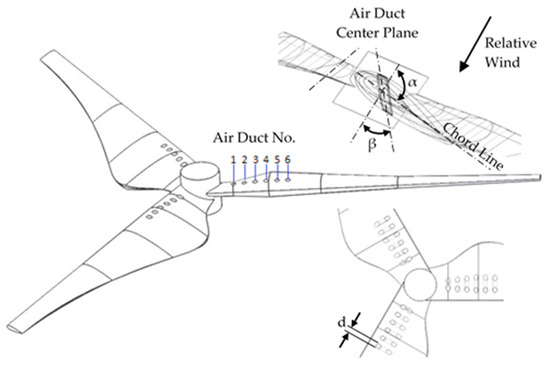
Figure 1.
Horizontal axis wind turbine with duct.
3. Numerical Study
The 3D calculation zone was created using ANSYS/Design Modeler software. It is important that the calculation zone is created as large as possible so that the results of the analysis are not affected by the limits of the calculation zone. However, it should be taken into consideration that this situation will increase the number of elements in the mesh structure of the model and the time of analysis. The calculation zone has a cylindrical shape and can be defined periodically for each blade. Therefore, a computational region was defined in which a single blade was located. On the other hand, considering that the Mach number value in the analyses was very small (0.018–0.023), the size independence study was performed, and the extents of the calculation area were determined depending on the rotor diameter. In practice, the calculation zone can be taken 10 times the diameter to ensure that the flow is fully developed when it comes to the blades, but this will greatly increase the calculation zone and, as it is, the number of elements in the analysis. Therefore, a parabolic speed entry limit requirement was defined to the model using expression, and 2 times the diameter was left from the entrance up to the blade. The length of the calculation zone will be taken 6 times the diameter so that the turbine back-flow part is not affected by the exit boundary condition.
Within the scope of CFD analysis, the air is assumed to be atmospheric condition. The velocity inlet and the pressure outlet boundary conditions were applied to the inlet surface and outlet surface, respectively. The rotating wall function was applied to the blade surface and to the rotor. Thus, the air flow at the computational domain boundary is not affected by non-slip condition on the outside wall boundary. The surface between inner-domain which covers the blade and outer-domain were defined as an interface, and the other surfaces as a periodic boundary condition. The computational domain and the boundary conditions depending on the rotor diameter was shown in Figure 2.
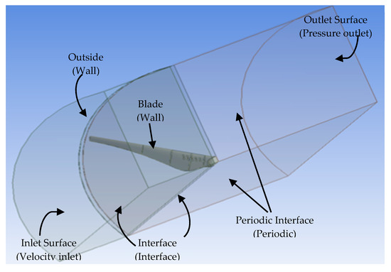
Figure 2.
3D periodic computational domain for single blade and boundary conditions.
For computational fluid dynamics (CFD) analyses a hexahedral type of cells should be preferred, given both the computational accuracy and the reduction of cell number. But due to the complex structure of the blade, a triangular pyramid mesh structure containing tetrahedron elements was used. The mesh structure must be proper in terms of the accuracy of the results. Therefore, it was sensitive to keeping the skewness values of the mesh to be created within the desired limits (0.50 ≤ skewness ≤ 0.80). However, the areas close to the blade surface where relatively precise calculations were needed, and the mesh structure around the ducts were composed of smaller elements than other regions by using a weight factor. In order to capture the airflow surface interaction and provide solution stabilization in these critical regions where reverse pressure gradients and serious speed changes occur, the boundary layer was used. First layer (4.3 × 10⁻⁵ m) and total layer thickness (2.2 × 10⁻³ m) were calculated as a function of the Reynolds number, chord and y+ value. Depending on the 1.2 growth rate, a 13-layer boundary layer was used [37,38].
The maximum, minimum and average skewness values of the mesh structure that make up the calculation zone were 0.91, 4.41 × 10⁻⁶ and 0.24, respectively. It can be said that the mesh structure is appropriate as the maximum skewness value of the mesh is below the maximum skewness value accepted in the literature, i.e., 0.98 [39]. On the other hand, the mesh structure contains 6054957 elements. Within the scope of the mesh sensitivity analysis, i.e., the size independence study, in which the change in the power coefficient was determined depending on the number of elements of the mesh, was performed. It was determined that the change in the power coefficient was below 1% when the number of mesh elements was over 6 million elements. After approximately 6 million elements, it was seen that increasing the number of elements has no significant effect on the results, so the analysis is independent of the mesh structure. Figure 3 shows the mesh structure used in CFD analysis.
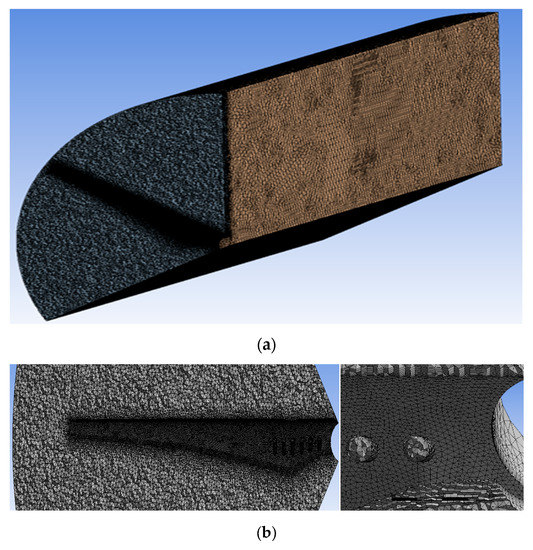
Figure 3.
(a) The mesh structure of the 3D model; (b) The mesh structure around of the blade and air ducts.
Continuity, momentum and turbulence equations for air-ducted blade model were solved with ANSYS/Fluent software, utilizing the pressure-based time-dependent formulation. As a turbulence model, k-epsilon RNG with a result of less than 5% error was preferred in horizontal-axis wind turbines [40]. In the turbulence model, y+ is preferred to be around 1 for an effective solution [39]. However, for the average grid (1 < y+ < 5) range, the turbulence model provides wall shear stress values compatible with experimental data [36]. Although the model does not reach y+ value of around 1, the maximum y+ value is about 4.
Due to the variety of rotational speed and the complexity of the flow field, determining an optimum time step for the transient solution is very difficult and sensitivity analysis is required. Especially at high speeds, the time step should be very small to capture turbulence on a small-time scale and to accurately simulate the rotation of the rotor. However, a very small-time step will result in a large increase in computation time. Besides, since the time step directly affects the numerical iteration process of the solver, large time steps will also produce non-physical results. Therefore, it is necessary to determine the optimum time step. For this purpose, many simulations were performed for different angular velocities and the time step value () for the first simulation was calculated from the following equation as a function of tip-speed ratio, air velocity, and blade length.
where is blade length, is tip-speed ratio, and is air velocity.
For the analysis with 6 m/s air velocity and with 7 tip-speed ratio, the initial time step value was calculated as 2.58 × 10⁻⁴ s. However, since the analyses performed with the initial time step value did not meet the convergence criteria and produced inappropriate bad results according to the experimental data, it was gradually decreased. With the help of sensitivity analysis, the optimum time step value was determined as 1.0 × 10⁻⁴ s.
The calculation zone was defined in atmospheric conditions. The mesh motion method, which allows angular velocity to be given to the blade and rotor, was used and, angular velocity was not given to the flow volume surrounding the blades. The mean moment coefficient () was used when calculating torque and power. The moment coefficient values of the turbine were monitored depending on the time until the turbine makes 10 cycles and the average moment coefficient was calculated from these data. The average torque () was calculated depending on airspeed and density, mean moment coefficient, turbine projection area, and chord () length. The power coefficient () was calculated as a function of torque data from the numerical model and angular velocity and the power of air coming into the turbine.
Within the scope of numerical calculations, flow velocity and pressure fields were obtained, and momentum, stability and pressure correction equations were solved respectively. In the early stages of the recursive solution procedure, a first order-upwind scheme was used to discriminate the convective terms and increase convergence. However, the final results were obtained using a second-order upwind scheme for better accuracy. To determine the convergence of analysis, not only the values obtained from the velocity field updated with the equations were not compared to the values obtained from the previous iteration, but also the variation of dimensionless numbers, highly effective on the aerodynamic characteristic of the blade such as lift and moment coefficient, was followed throughout iterations. It was decided that the values obtained from the speed field provided convergence criteria (>0.001) and that analyses converged under conditions where the dimensionless numbers that were followed were no longer changed by iterations. Verification experiments were conducted to prove the reliability of the results obtained from analyses. The CFD analysis was performed for 58 hours using a 12-core workstation with 32 GB DDR4 RAM.
Validation
The experimental study was carried out to confirm the numerical model. In the test setup, the quad fan (Axial fan, BVN-BSV-750, 17,400 m3/h) was used as the source of airflow. Flow-straightener was used to smooth the flow. The data of the airflow generated in the experimental setup was measured with a digital anemometer (Lutron AM-4206). An optical non-contact tachometer (Uni-T UT372) was used to obtain the turbine speed. 3 phase AC permanent magnet generator (Nominal power 300 W) was used in the wind turbine. Current (I) and voltage (V) produced by the generator were measured by two separate digital multimeters (Brymen BM525s) to obtain the output power of the wind turbine. The data measured during the experiment were transferred to the computer simultaneously. The experimental setup is shown in Figure 4.
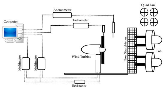
Figure 4.
Experimental setup.
Although the measured power curve was determined by utilizing simultaneous wind speed and power output data, the key element of the power performance testing was the measurement of wind speed. The position of the anemometer’s probe is extremely important so that the wind speed is not affected and the correlation between wind speed and electrical power output does not decrease. The anemometer probe can be located at a distance from the wind turbine 2 to and 4 times of the rotor diameter (D). For horizontal axis wind turbines, this distance is recommended to be 2.5D. The anemometer should be mounted as close as possible to the centerline of the turbine rotor, not more than 0.2H from the centerline where H is the turbine hub height [41].
Within the scope of analyses, the angle of attack of the blade, the diameter, inclination, and number of the air duct were taken as parameters to determine the best blade design to give high performance to the wind turbine made of composite material (Epoxy-glass) with a blade length of 0.62 m, a rotor diameter of 1.26 m and a sweeping area of 1.21 m2, at wind speed of 6–8 m/s (average wind speed found by various studies). To determine the reliability of the results obtained from analyses, validation experiments were conducted for wind turbines with air ducted and duct-free blades. The average power coefficient () obtained from the wind turbine depending on the electrical and wind power was defined in Equation (4).
where is the angular position of the wind turbine, is the electrical power generated by the generator depending on the angular position, is wind power, n is the number of time steps in which the turbine returns to complete around, and is the generator efficiency. Mechanical losses were neglected as the moment was transferred directly to the generator with a short shaft without using any gear system. Uncertainty analysis was performed for measurements carried out within the scope of the experimental study. When determining the power coefficient, the error rate was determined as ±2.2% using Equation (5) depending on the measurements of current (I; 0.2% + 4d, Brymen BM525s), voltage (V; 0.08% + 2d, Brymen BM525s) and wind speed (±2% + 0.2 m/s, Lutron AM-4206). Furthermore, while the blade tip velocity rate was determined, the error rate encountered based on wind speed and angular velocity (±0.04% + 2, UNI-T UT 372) measurements were found as ±3.6% by using Equation (6).
where is error in power measurement and is error in tip-speed ratio measurement.
A comparison of the power coefficient values obtained from experimental studies and CFD analyses is shown in Figure 5. The average value obtained from the experiments for each tip-speed ratio is shown in the graph. It is observed that curves formed for the experimental data are compatible with the CFD results. The results showed a 5.3% error in low blade tip-speed rates, while increased by up to 6.8% in high tip-speed rates. Due to the complexity of the flow field, relatively higher error rates occurred at higher speeds, because the numerical model captures the airflow surface interaction and flow separation relatively poor at high speeds.
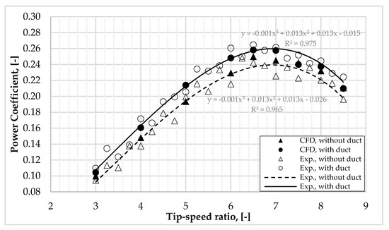
Figure 5.
Comparison of the experimental study and CFD analysis results performed at 6 m/s air velocity and 7 tip-speed ratio.
4. Results and Discussion
To compare the effect of air ducts, i.e., the new design proposed in this study, CFD analyses of air duct-free blade was performed at different angle of attacks. For the blade tip-speed ratio of 7, the obtained power coefficient values depending on the angle of attack at different wind speeds ranging from 6 m/s to 8 m/s are shown in Figure 6. An increase in the angle of attack results in an increase in the lift coefficient, which directly affects power coefficient, up to a critical point which is known as an aerodynamic stall point. After the angle of attack exceeds this critical point, the airflow across the upper surface of the blade becomes detached. Therefore, the lift coefficient is dramatically decreased. In the wind speed range, which is aimed to improve the blade performance, relatively high-power coefficient values were obtained between 5° and 8° angles of attack for air duct-free blade design. Under the critical air velocity at which the local boundary layer on the upper surface of the blade begins to separate, the increase in the velocity increases the kinetic energy of the airflow and delays the boundary layer separation from the surface. Therefore, as seen in Figure 6, the aerodynamic stall point has been shifted to larger angle of attacks due to the increase in air velocity.
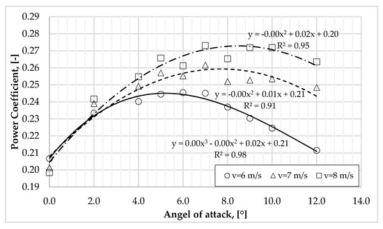
Figure 6.
Power coefficient values based on the angle of attack at different airspeeds for air duct-free blade design.
To determine the effects of optimization parameters on the power coefficient, analyzes were performed by changing only one parameter at a time. The obtained results were compared with the situation where there are no air ducts and the maximum and minimum values that the parameters can take during the optimization process were determined. While the power coefficient values obtained depending on the duct slope are given in Table 2, the power coefficient values obtained depending on the duct diameter are given in Table 3. For all airspeed values, the greater power coefficient was obtained for the 35°, 40°, and 45° values of the slope of the channel. Besides, when compared to the without duct design, greater power coefficient values were obtained from the design with a duct diameter ranging from 14 mm to 26 mm.
Table 2.
Power coefficient values depending on duct slope for airspeed values 6, 7, and 8 m/s on the 6-ducted blade with the 7° angle of attack.
Table 3.
Power coefficient values depending on duct diameter for airspeed values 6, 7, and 8 m/s on the 6-ducted blade with the 7° angle of attack and 35° duct slope.
In the optimization study, the optimum parameter values for air ducted blade design at 7° angle of attack were 18 mm, 35° and 6, for duct diameter, slope, and number, respectively. Figure 7 shows power coefficient values and maximum power curves based on various blade tip-speed ratio from air ducted and duct-free blade designs at wind speeds of 6, 7 and 8 m/s. The aerodynamic stall occurred at tip-speed ratio values in the range of 7 to 8 for the air speeds where the analyzed were performed. When the maximum power curves of air ducted and duct-free blade designs were examined, it was determined that the air ducts on the blade increased the power coefficient by 2.2–4.4%.
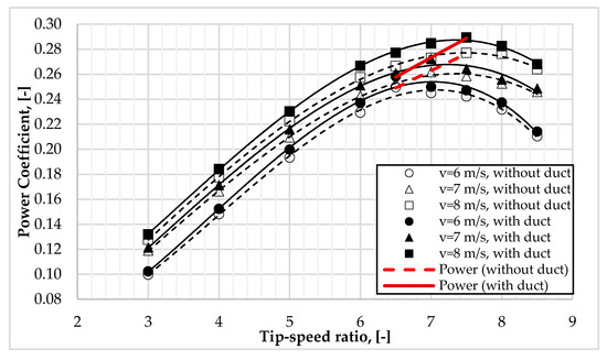
Figure 7.
Power coefficients and maximum power curves obtained from the blade, which is designed with and without air ducts at various wind speeds, depending on the blade tip-speed ratio.
When the critical wind speed, which varies depending on the shape parameters of the blade, is exceeded, local boundary layer separations occur on the blade. Thus, the turbine produces low power, especially at high wind speeds. With the air ducts on the blade, sufficient momentum is transferred to the boundary layer to prevent flow separation, and by increasing the kinetic energy of the low-momentum fluid in the area close to the surface, the boundary layer separation from the surface is delayed.
The streamlines on the blade profile and the kinetic energy gradient in the blade profile section are shown in Figure 8 and Figure 9, respectively. In the air ducted blade design, the extra airflow from the ducts increases the kinetic energy of the low momentum airflow on upper surface of the blade profile, thereby delaying the separation of the flow (yellow mark). This allows the blade to run longer at the high-power coefficient. Under the same conditions, it appears that flow separation occurs on the upper surface of the blade profile (red mark), which does not have air ducts.
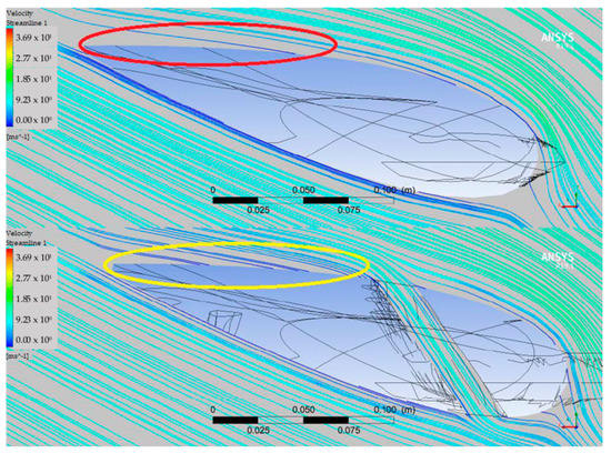
Figure 8.
Streamlines in the blade profile section.
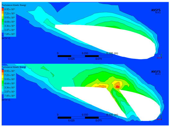
Figure 9.
Turbulence kinetic energy in the blade profile section.
In Figure 10, the pressure differential values between the inlet and outlet of the air ducts are shown comparatively for air ducted and duct-free blade designs. The pressure difference in the first three ducts of the 6-duct blade design is greater than the duct-free blade profile, while from the 4th duct, the pressure difference value is higher in the duct-free blade profile. Considering that the pressure difference on the blade is directly related to the pressure forces and the torque value that can be obtained from the blade and that this change in torque will be greater in areas away from the root where the blade speed is relatively high, this situation indicates the existence of a critical number of ducts. Air ducts on the blade increase the wall shear forces, as well as significantly reducing pressure forces after a critical number of ducts. Also, after the critical number of ducts, the gain from the peripheral shift forces cannot supply the loss of pressure forces and the blade loses power. Therefore, determining the optimum number of air ducts is very important. The critical number of ducts was determined to be 6 for 7° angle of attack, 18mm duct diameter, and 35° duct slope.
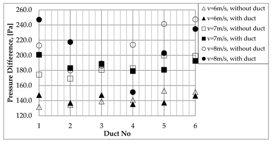
Figure 10.
Maximum pressure differences between the inlet and outlet of the air ducts.
5. Conclusions
In this study, a new blade design has been developed to increase wind turbine efficiency. To obtain maximum power from the A-DB design, the Response Surface Optimization method was used to determine the optimum values of parameters, such as duct diameter, slope, number and angle of attack of the blade. Thus, a targeted optimization was made that provides the best possible design according to the constraints and targets set for the optimization parameters.
Opening the air ducts on the blade increases the viscous forces while decreasing the pressure forces. To minimize the effect of the decrease in pressure forces, the air ducts were located in the max chord section which is near the root section of the blade. Considering that the pressure forces are more effective than the viscous forces on the total force, a critical number of ducts should be defined. Because of the increase in the number of air ducts after a critical value, the increase in the force from the viscous forces cannot compensate for the decrease in the force to be lost from the pressure forces. Although the number of critical ducts varies depending on the shape parameters, angle of attack and wind speed, the 6-ducted blade design has come into prominence with 7° angle of attack in CFD analysis.
With the passive flow control method, a sufficient amount of momentum is transferred to the area where the air ducts are located, and the airflow is attached to the upper surface of the blade. Thus, the blade is provided to work longer with the maximum power coefficient. This may provide a serious increase in the annual electricity production (AEP) of the wind turbine.
According to the results obtained from CFD analysis, the air ducts added on the blade increased the power coefficient between 3.4% and 4.4% depending on the wind speed. Considering that the highest theoretically achievable aerodynamic efficiency of turbine blades, known as the Betz limit, is approximately 59% and that the medium-sized commercial horizontal-axis turbines operate at approximately 25–35% efficiency, this would be regarded as a significant increase.
According to the literature, rotor performance can be increased by active flow control such as pitch and yaw control. However, in this study, without an external energy input into the system, the performance was increased with passive flow control by utilizing air ducts. This will reduce the annual energy consumption of the wind turbine.
In addition to the development of the existing parameters, further studies can be carried out to reach higher power coefficient values by enriching the parameters of the air duct, such as using different duct shapes and reducing the diameter of the duct from the inlet to the exit. Besides, considering the potential of the horizontal axis wind turbine blades to produce vibrations, the effects of air ducts on both the structural strength of the blade and the noise level produced by the turbine can be examined within the scope of future studies.
6. Patent
The air duct blade design of the horizontal axis wind turbine used in this study has been patented by the Turkish Patent and Trademark Office with the number of TR-2016-06156B.
Funding
This research received no external funding.
Conflicts of Interest
The authors declare no conflict of interest.
Abbreviations
| A-DB | Air Ducted Blade |
| AEP | Annual Electricity Production |
| BEM | Blade Element Momentum Theory |
| CFD | Computational Fluid Dynamic |
| CFDDA | Climate Four-Dimensional Data Assimilation |
| DOE | Design of Experiment |
| HAWT | Horizontal Axis Wind Turbine |
| MERRA | Modern-Era Retrospective Analysis |
| MOGA | Multi-Objective Genetic Algorithm |
| NLPQL | Non-Linear Programming by Quadratic Lagrangian |
| RNG | Re-Normalization Group |
| RSO | Response Surface Optimization |
| TSR | Tip-Speed Ratio |
References
- Saundry, P.D. Review of the United States energy system in transition. Energy Sustain. Soc. 2019, 9, 4. [Google Scholar] [CrossRef]
- Raheem, A.; Abbasi, S.A.; Memon, A.; Samo, S.R.; Taufiq-Yap, Y.H.; Danquah, M.K.; Harun, R. Renewable energy deployment to combat energy crisis in Pakistan. Energy Sustain. Soc. 2016, 6, 1–13. [Google Scholar] [CrossRef]
- Maalawi, K.W.; Badawy, M.T.S. A direct method for evaluating performance of horizontal axis wind turbines. Renew. Sustain. Energy Rev. 2001, 5, 175–190. [Google Scholar] [CrossRef]
- Xudong, X.; Shen, W.Z.; Zhu, W.J.; Sorensen, J.N.; Jin, C. Shape optimization of wind turbine blades. Wind Energy 2009, 12, 781–803. [Google Scholar] [CrossRef]
- Xu, L.; Xu, L.; Zhang, L.; Yang, K. Design of wind turbine blade with thick airfoils and flat back and its aerodynamic characteristic. Open Mech. Eng. J. 2015, 9, 910–915. [Google Scholar] [CrossRef]
- Lee, M.H.; Shiah, Y.C.; Bai, C.J. Experiments and numerical simulations of the rotor-blade performance for small-scale horizontal axis wind turbine. J. Wind Eng. Ind. Aerodyn. 2016, 149, 17–29. [Google Scholar] [CrossRef]
- Lanzafame, R.; Messinai, M. Power curve control in micro wind turbine design. Energy 2010, 35, 556–561. [Google Scholar] [CrossRef]
- Pourrajabian, A.; Nazmi Afshar, P.A.; Ahmedizadeh, M.; Wood, D. Aero-structural design and optimization of a small wind turbine blade. Renew. Energy 2016, 87 (Pt 2), 837–848. [Google Scholar] [CrossRef]
- Ashrafi, Z.N.; Ghaderi, M.; Sedaghat, A. Parametric study on off-design aerodynamic performance of a horizontal axis wind turbine blade and proposed pitch control. Energy Convers. Manag. 2015, 93, 349–356. [Google Scholar] [CrossRef]
- Jureczko, M.; Pawlak, M.; Mezyk, A. Optimization of wind turbine blades. J. Mater. Process. Technol. 2005, 167, 463–471. [Google Scholar] [CrossRef]
- Rehman, S.; Alam, M.D.M.; Alhems, L.M.; Rafique, M.M. Horizontal axis wind turbine blade design methodologies for efficiency enhancement. Energies 2018, 11, 506–540. [Google Scholar] [CrossRef]
- Mahdi, N.A.; Farzad, M.; Mehdi, S. Performance improvement of a wind turbine blade using a developed inverse design method. Energy Equip. Syst. 2016, 4, 1–10. [Google Scholar] [CrossRef]
- Karthikeyan, N.; Kalidasa, M.K.; Arun, K.S.; Rajakumar, S. Review of aerodynamic developments on small horizontal axis wind turbine blade. Renew. Sustain. Energy Rev. 2015, 42, 801–822. [Google Scholar] [CrossRef]
- Duquette, M.M.; Visser, K.D. Numerical implications of solidity and blade number on rotor performance of horizontal-axis wind turbine. J. Sol. Energy Eng. 2003, 125, 425–432. [Google Scholar] [CrossRef]
- Ponta, F.L.; Otero, A.D.; Lago, L.I.; Rajan, A. Effects of rotor deformation in wind-turbine performance: The dynamic rotor deformation blade element momentum model (DRD-BEM). Renew. Energy 2016, 92, 157–170. [Google Scholar] [CrossRef]
- Wang, J.; Qin, D.; Lim, T.C. Dynamic analysis of horizontal axis wind turbine by thin-walled beam theory. J. Sound Vib. 2010, 329, 3565–3586. [Google Scholar] [CrossRef]
- Tummala, A.; Velamati, R.K.; Sinha, D.K.; Indraja, V.; Krishna, V.H. A review on small scale wind turbines. Renew. Sustain. Energy Rev. 2016, 56, 1351–1371. [Google Scholar] [CrossRef]
- Scappatici, L.; Bartolini, N.; Castellani, F.; Astolfi, D.; Garinci, A.; Pennicchi, M. Optimizing the design of horizontal-axis small wind turbines: From the laboratory to market. J. Wind Eng. Ind. Aerodyn. 2016, 154, 58–68. [Google Scholar] [CrossRef]
- Villalpando, F.; Reggio, M.; Ilinca, A. Numerical study of flow around iced wind turbine airfoil. Eng. Appl. Comput. Fluid Mech. 2012, 6, 39–45. [Google Scholar] [CrossRef]
- Baxevanou, C.A.; Fidaros, D.K. Validation of numerical schemes and turbulence models combinations for transient flow around airfoil. Eng. Appl. Comput. Fluid Mech. 2008, 2, 208–221. [Google Scholar] [CrossRef]
- Fatehi, M.; Nili-Ahmadabadi, M.; Nematollahi, O.; Minaieah, A.; Kim, K.C. Aerodynamic performance improvement of wind turbine blade by cavity shape optimization. Renew. Energy 2019, 132, 773–785. [Google Scholar] [CrossRef]
- Seo, S.; Hong, C. Performance improvement of airfoils for wind blade with groove. Int. J. Green Energy 2016, 13, 34–39. [Google Scholar] [CrossRef]
- Liu, H.; Yu, Y.; Chen, H.; Yu, M.; Zang, D. A parametric investigation of endwall vortex generator jet on the secondary flow control for a high turning compressor cascade. J. Therm. Sci. Technol. 2017, 12. [Google Scholar] [CrossRef]
- Sundaravadivel, T.A.; Pillai, S.N.; Kumar, C.S. Influence of boundary layer control on wind turbine blade aerodynamic characteristic–Part I–Computational Study. In Proceedings of the 8th Asia-Pacific Conference on Wind Engineering (APCWE-VIII), Chennai, India, 10–14 December 2013; pp. 1211–1217. [Google Scholar]
- Chishty, M.A.; Hamdani, H.R.; Parvez, K. Effect of turbulence intensities and passive flow control on LP turbine. In Proceedings of the 10th International Bhurban Conference on Applied Science&Technology (IBCAST), Islamabad, Pakistan, 15–19 January 2013. [Google Scholar] [CrossRef]
- Fernandez-Gamiz, U.; Zulueta, E.; Boyano, A.; Ansoategui, I.; Uriarte, I. Five-megawatt wind turbine power output improvements by passive flow control devices. Energies 2017, 10, 742–757. [Google Scholar] [CrossRef]
- El-Gendi, M.M.; Ibrahim, M.K.; Mori, K.; Nakamura, Y. Novel flow control method for vortex shedding of turbine blade. Trans. Jpn. Soc. Aero. Space Sci. 2010, 53, 122–129. [Google Scholar] [CrossRef]
- Seifert, A.; Stalnov, O.; Troshin, V.; Avnaim, M.H. On the application of active flow control to wind turbines. In Proceedings of the Fluids Engineering Division Summer Meeting, Hamamatsu, Japan, 24–29 July 2011; pp. 3057–13006. [Google Scholar]
- Cortesi, N.; Torralba, V.; Gonzalez-Reviriego, N.; Soret, A.; Doblas-Reyes, F.J. Characterization of European wind speed variability using weather regimes. Clim. Dyn. 2019, 53, 4961–4967. [Google Scholar] [CrossRef]
- Hasager, C.B.; Vincent, P.; Badger, J.; Badger, M.; Di Bella, A.; Pena, A.; Husson, R.; Volker, P.J.H. Using satellite sar to characterize the wind flow around offshore wind farms. Energies 2015, 8, 5413–5439. [Google Scholar] [CrossRef]
- Global Wind Atlas, Mean Wind Speed at 100 m above the Surface. Available online: http://science.globalwindatlas.info/datasets.html (accessed on 21 April 2020).
- Prince, S.A.; Badalamenti, C.; Regas, C. The application of passive air jet vortex-generators to stall suppression on wind turbine blades. Wind Energy 2017, 20, 109–123. [Google Scholar] [CrossRef]
- Cengel, Y.A.; Cimbala, J.M. Fluid Mechanics: Fundemental and Applications, 3rd ed.; McGraw-Hill Companies: New York, NY, USA, 2013. [Google Scholar]
- Kapitler, M.; Kokalj, F.; Samec, N. Numerical optimisation of operating conditions of waste to energy. WIT Trans. Ecol. Environ. 2010, 140, 31–41. [Google Scholar] [CrossRef]
- Mandloi, P.; Verma, G.; Boland, A. Design optimization of an in-cylinder engine intake port. In Proceedings of the NAFEMS Word Congress’09 (NWC-2009), Crete, Greece, 16–19 June 2009. [Google Scholar]
- Yigit, C. Wind Turbine Blade Design with Air-Ducted. National Patent, Patent No: TR-2016-06156B, 21 November 2019. (In Turkish). [Google Scholar]
- Salih, S.Q.; Aldlemy, M.S.; Rasani, M.R.; Ariffin, A.K.; Tuan Ya, T.M.Y.S.; Al-Ansari, N.; Yaseen, Z.M.; Chau, K.W. Thin and sharp edges bodies-fluid interaction simulation using cut-cell immersed boundary method. Eng. Appl. Comput. Fluid Mech. 2019, 13, 860–877. [Google Scholar] [CrossRef]
- Ghalandari, M.; Bornassi, S.; Shamshirband, S.; Mosavi, A.; Chau, K.W. Investigation of submerged structures’s flexibility on sloshing frequency using a boundary element method and finite element analysis. Eng. Appl. Comput. Fluid Mech. 2019, 13, 519–528. [Google Scholar] [CrossRef]
- Ansys, Fluent User Guide. Available online: https://support.ansys.com/portal/site/AnsysCustomerPortal (accessed on 2 April 2020).
- Yigit, C. Improving the horizontal axis wind turbine blade profiles. Sak. Univ. J. Sci. 2018, 22, 1432–1437. [Google Scholar] [CrossRef]
- IEC61400-12-1 (2.0b). Wind Turbines–Power Performance Measurement of Electricity Producing Wind Turbine, 2nd ed.; IEC: Geneva, Switzerland, 2017. [Google Scholar]


© 2020 by the author. Licensee MDPI, Basel, Switzerland. This article is an open access article distributed under the terms and conditions of the Creative Commons Attribution (CC BY) license (http://creativecommons.org/licenses/by/4.0/).