Unsteady Natural Convection in a Cylindrical Containment Vessel (CIGMA) With External Wall Cooling: Numerical CFD Simulation

Abstract

In the case of a severe accident, natural convection plays an important role in the atmosphere mixing of nuclear reactor containments. In this case, the natural convection might not in the steady-state condition. Hence, instead of steady-state simulation, the transient simulation should be performed to understand natural convection in the accident scenario within a nuclear reactor containment. The present study, therefore, was aimed at the transient 3-D numerical simulations of natural convection of air around a cylindrical containment with unsteady thermal boundary conditions (BCs) at the vessel wall. For this purpose, the experiment series was done in the CIGMA facility at Japan Atomic Energy Agency (JAEA). The upper vessel or both the upper vessel and the middle jacket was cooled by subcooled water, while the lower vessel was thermally insulated. A 3-D model was simulated with OpenFOAM^®, applying the unsteady Reynolds-averaged Navier–Stokes equations (URANS) model. Different turbulence models were studied, such as the standard k-ε, standard k-ω, k-ω shear stress transport (SST), and low-Reynolds-k-ε Launder–Sharma. The results of the four turbulence models were compared versus the results of experimental data. The k-ω SST showed a better prediction compared to other turbulence models. Additionally, the accuracy of the predicted temperature and pressure were improved when the heat conduction on the internal structure, i.e., flat bar, was considered in the simulation. Otherwise, the predictions on both temperature and pressure were underestimated compared with the experimental results. Hence, the conjugate heat transfer in the internal structure inside the containment vessel must be modeled accurately.

1. Introduction

Natural convection heat transfer in the cavity of the enclosure is an important research topic due to its wide range of engineering applications, such as the energy-efficient design of buildings [1], electronic devices [2], solar energy [3], operation and safety of nuclear reactors [4], etc. In nuclear reactors, natural convection is utilized as long-term passive containment cooling during an accident. In the case of a postulated light water reactor accident, e.g., loss of coolant accident (LOCA), natural convection plays a vital role as an inherent safety function in order to reduce the pressure and temperature in the containment vessel [5]. Therefore, investigations on the natural convection related to gas transport and mixing in a containment vessel have become an important research topic to determine hydrogen-related risks [6].

The Fukushima nuclear accident underlines the importance of providing countermeasures against the risks of fission products (FPs) release and hydrogen explosion under severe accidents. Hence, several international projects related to the nuclear containment thermohydraulic have been studied in different research facilities. In the THAI facility (Becker Technologies, Germany), experiment tests TH21, TH22, and TH24 were performed to simulate the natural convection through differential heating and cooling of the vessel walls [6,7]. Later, the experimental data on TH21, TH22, and TH24 were used for numerical validation by means of computational fluid dynamics (CFD) and lumped parameter (LP) codes [8,9]. In the MISTRA facility (CEA, France), the natural convection experiment (NATHCO) in the framework OECD SETH-2 project was performed [10]. It consisted of gradually heating condensers, installed near the vessel wall, to heat the nearby gas and induce buoyant flow in the stagnant atmosphere.

The vast majority of the numerical studies on natural convection in the containment vessel are based on the unsteady Reynolds-averaged Navier–Stokes (URANS) simulations [11,12]. The URANS model is commonly used due to the lower computational cost compared with the scale-resolving simulations, such as LES and hybrid RANS/LES. The accuracy of the URANS simulations, however, strongly depends on the computational settings. Previous studies have shown the important impact of the grid size, turbulence models, and boundary conditions [13]. Visser et al. [13] simulated natural convection in the containment vessel using commercial CFD ANSYS Fluent. Basically, the default numerical schemes of the applied code ANSYS Fluent were applied, i.e., spatial discretization was second-order upwind and the temporal discretization on the second-order Euler backward scheme. The obtained results indicated that the variation of the numerical results obtained using the k–ε turbulence model was small, whereas the standard k-ω turbulence model with the effect of buoyancy on k included still predicts a higher dissolution rate. In this case, the SST k–ω turbulence model with the effect of buoyancy on k had the best overall performance. They also concluded that the mesh size 45 mm × 75 mm in bulk was sufficiently small to model the natural convection in the containment vessel.

However, to the best of our knowledge, no systematic investigation has been performed to critically assess the effectiveness of the internal structure inside a containment vessel on the overall heat transfer. Therefore, the accuracy of the numerical models, i.e., conjugate heat transfer model in comparison to experiments, should be performed to identify the best-performing models for CFD simulations. This indicates the need for more extensive sensitivity analyses to support CFD studies of a natural convention in the containment vessel.

In the previous study [11,12], the natural convection in the containment vessel was achieved by prescribing steady thermal boundary conditions (BCs) on either a cooled or heated wall. However, the steady natural convection might not have occurred in the case of a postulated light water reactor accident. The unsteady natural convection might have happened inside the containment vessel when the accident mitigation, e.g., externally flood the primary containment vessel (PCV) or drywell (DW) head using portable pumps or other means, is activated during the accident [14,15]. Therefore, the unsteady thermal boundary conditions on the containment should be addressed to understand the phenomena and processes of unsteady natural convection, which may occur during the accident.

Our final goal was to validate the numerical simulation of unsteady natural convection inside the containment vessel in case of an accident scenario. Thus, the natural convection of the high temperature of steam and non-condensable gas should be performed experimentally and numerically. However, in the present stage, heated air was the only gas used in the experiment. In Japan Atomic Energy Agency (JAEA), the Rig of Safety Assessment–Severe Accident (ROSA-SA) project was initiated to study the containment of thermal-hydraulics related to over-temperature containment damage, hydrogen risk, and fission product transport [16]. One of the research facilities in JAEA for the integral test is a Containment InteGral Measurement Apparatus (CIGMA). The CIGMA facility is equipped with external cooling on the containment wall. The natural convection experiment series was done in the CIGMA facility [17,18].

The experiment on the unsteady natural convection of air around a cylindrical containment with unsteady thermal BCs at the vessel wall was performed. The upper vessel or both the top vessel and the middle jacket were cooled by subcooled water, while the lower vessel was thermally insulated. Later, the numerical analysis was performed using the data of those experiments. A 3-D model was simulated with OpenFOAM^®, applying the unsteady Reynolds-averaged Navier–Stokes equations (URANS) model. The performance of a high Reynolds number and a low Reynolds number turbulence model was assessed to select the most appropriate turbulence model for natural convection modeling in the large containment vessel.

In the present study, the results obtained by the high Reynolds number and a low Reynolds number turbulence models were compared against the results of the experimental data. The test data on the previous publication (TH24 test) revealed that the wall temperature of the inner cylinder is governed by the thermal inertia of the structure itself [8]. In addition, flat bars that were used to fix the measurement instrumentations, such as the thermocouple and capillary tube, which were simulated in order to know their effect on the overall heat transfer. The internal structure of the CIGMA facility, i.e., flat bars, was modeled by employing the conjugate heat transfer. All models predict the pressure and temperature inside the containment vessel, which are also shown and discussed in this paper.

2. Experimental Apparatus (CIGMA) and Procedure

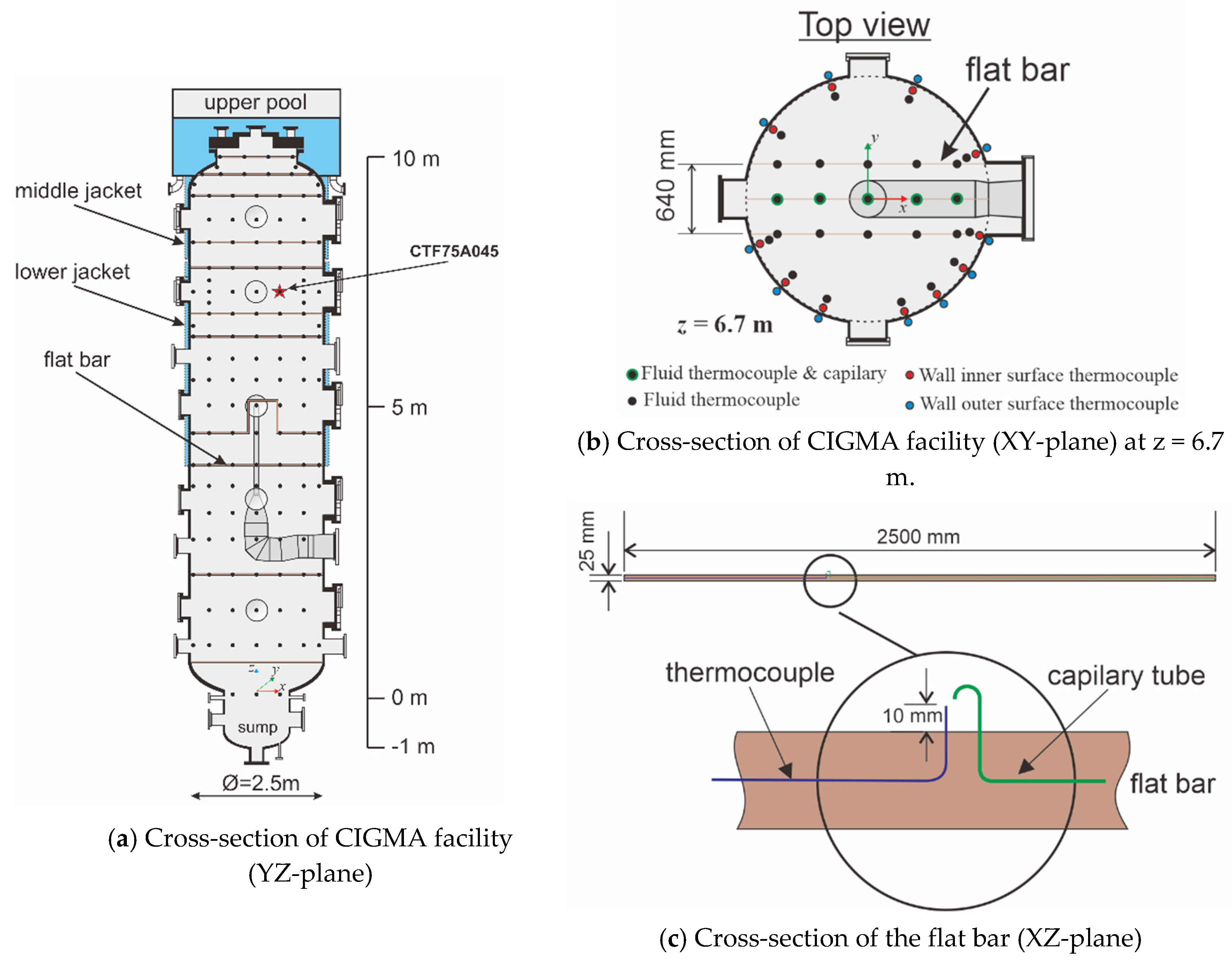
2.1. CIGMA Facility

The detailed description of the CIGMA facility and its components can be seen in the previous publications [19,20]. Figure 1a shows the schematic view of CIGMA facility at JAEA. The CIGMA facility is a large cylindrical stainless-steel vessel with an inner diameter of the main cylindrical part of 2.5 m and an overall inner height of 11 m. The vessel wall is thermally isolated using rock-wool mats covered by reinforced wire mesh and equipped with three external water-cooling systems, i.e., upper pool, middle jacket, and lower jacket. In the present experiments, the upper pool and middle jacket were used for the external surface cooling. The temperature and pressure boundary of the containment vessel can only withstand up to 300 °C and 1.5 MPa. The test section of CIGMA has a large number of thermocouples (TCs), i.e., 650 TCs and capillary tubes (CTs), i.e., 100 CTs for the measurement of the temperature and gas concentration. The thermocouples are K-type, and they are arrayed like a grid. The positions of the thermocouples and capillary tubes are indicated by small dots, as shown in Figure 1a. It means that the CIGMA facility is equipped with high spatial resolution instrumentation, and the experiments provide suitable data for CFD validation.

The flat bars, as shown in Figure 1b, are installed inside the vessel to fix the thermocouples and capillary tubes. The location of the thermocouples for fluid temperature measurement is depicted as a black circle. Additionally, thermocouples are installed on the wall surface to monitor the wall temperature. A pair of thermocouples on the inner wall surface, i.e., red circle and outer wall surface, i.e., green circle, are installed at the same position across the wall. This configuration allows us to estimate a heat flux through the wall. The thickness of the flat bar is relatively small, i.e., 4 mm, thus its disturbance on the flow is minimized. The effect of flat bars on the flow behavior was negligible, as reported in the previous work [20]. Figure 1c shows the cross-section of the flat bars. The thermocouples are suspended within the gas and directly measure the gas temperature. It can be seen that the tip of the thermocouple (purple line) is located 10 mm above the edge of the flat bar. The distance between the two tips, i.e., between the temperature and concentration measurement locations, is set to be 5 mm or less. The radiation heat loss on the thermocouple to the solid surrounding wall was not considered due to the experiment being conducted at relatively low temperatures (T < 600 K). Otherwise, the radiation heat transfer should be included when the temperature is up to 600 K [21,22].

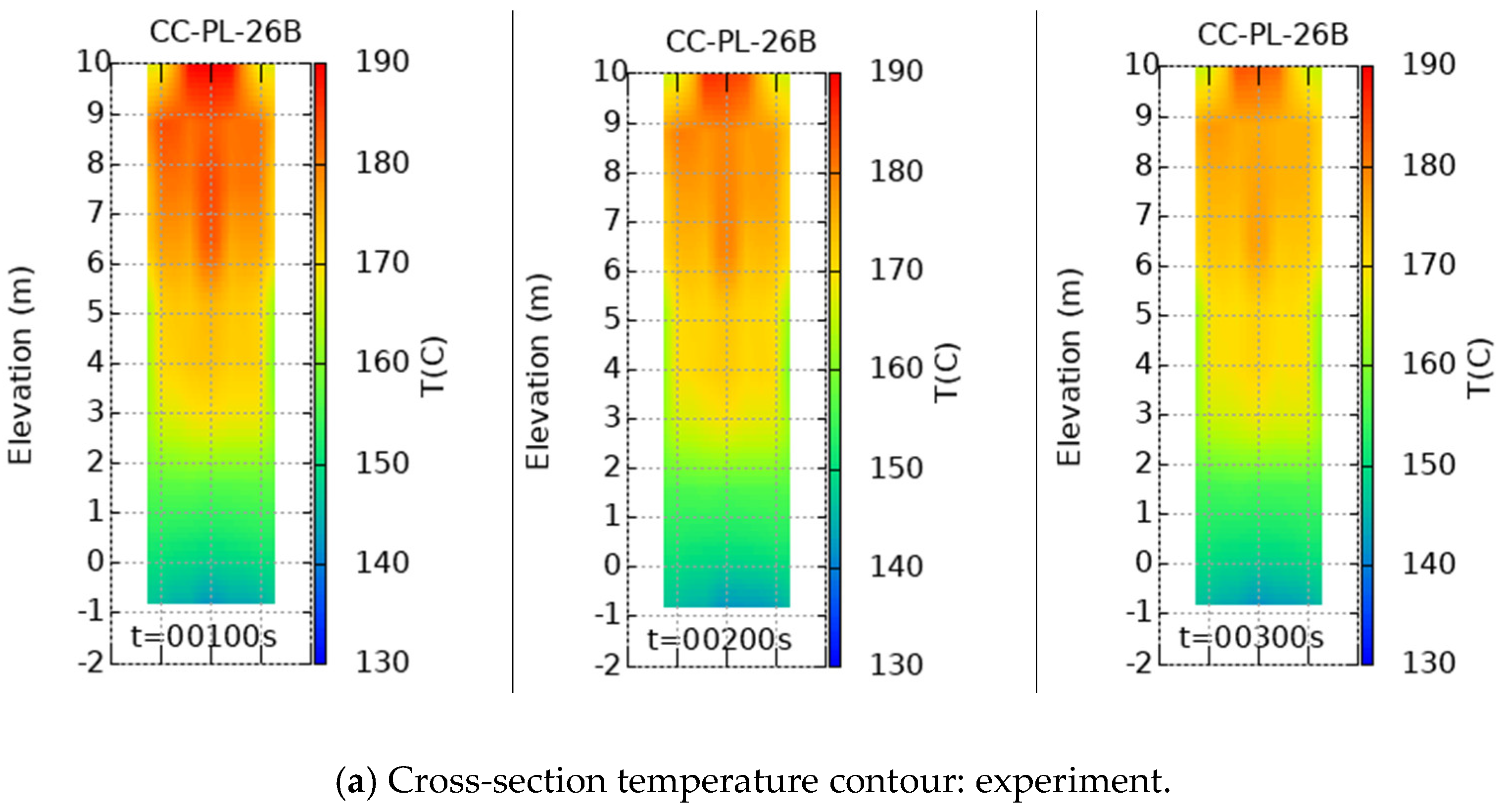
2.2. Natural Convection in the CIGMA Containment Vessel (CC-PL-26B)

The experimental conditions of natural convection in the CIGMA vessel are summarized in

Table 1. Experimental conditions.

Parameter	Run ID: CC-PL-26B
Average air temperature inside the vessel	T (K)	450
Average air pressure inside the vessel	P (kPa)	185
Cooling region	-	upper pool, middle jacket
Average water temperature in the upper pool and middle jacket	T (K)	303
Initiation of water injection into upper pool and middle jacket	t (s)	300
Timespan of the experiment	t (s)	4000

. The test vessel of the CIGMA facility was preheated by the injection of heater air. The preheating process is mainly used to heat the solid steel structures. The heated air injection was stopped after the pressure and temperature attained a specific initial condition. The temperature and pressure inside the vessel were monitored to ensure that the quasi-steady state was reached before the surface cooling was initiated. The surface cooling the vessel by subcooled water was started at t = 300 s. The coolant water was poured into the upper pool and stopped when the top flange of the vessel was fully flooded by water. The temperature and pressure inside the containment vessel were monitored and recorded for about 4000 s. Then, the experiment was stopped when there was no significant change in the pressure and temperature.

3. CFD Modeling and Numerical Approach

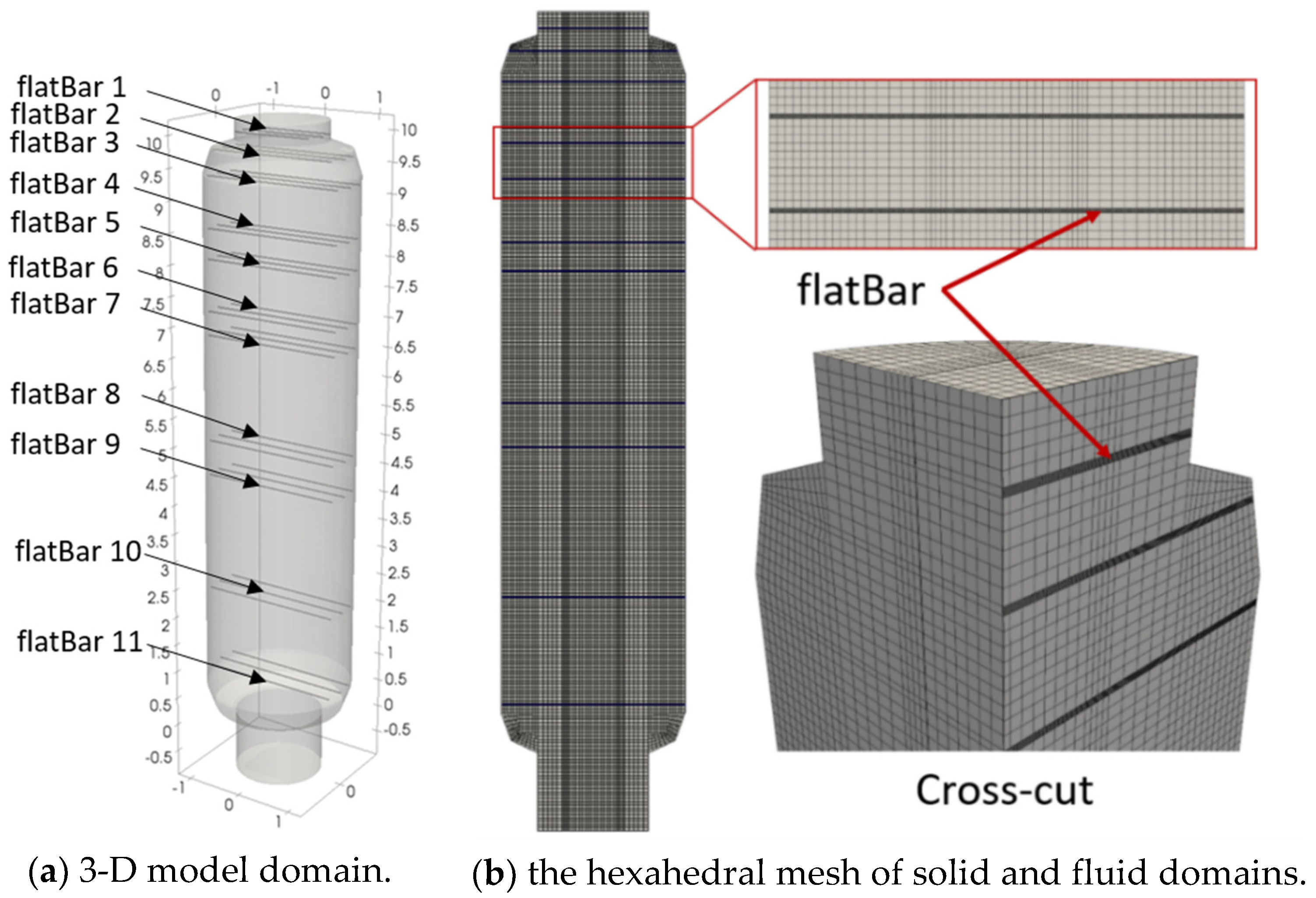
3.1. 3-D containment Vessel (CIGMA): Geometry and Mesh

A 3-D model domain is shown in Figure 2a. The fluid and solid domains were discretized by structured hexahedral mesh, as shown in Figure 2b. The O-grid topology was used to generate the model domain. The advantage of the O-grid topology is that it is possible to remove the highly skewed cells for a circular cylinder. Therefore, a structured mesh can be generated, and it offers simplicity and efficiency. The mesh was generated with ANSYS mesh CFD software and then exported to OpenFOAM. The flanges, nozzles, and solid walls were not discretized in order to simplify the model geometry and also for the ease in making hexahedral cells. Hence, the heat conduction in the solid wall was not taken into account. The flat bar was the only internal structure that was discretized in the present analysis. The cell size on the flat bar or the solid domain is smaller than the fluid domain, and its minimum size is 5 mm × 5 mm × 5 mm in the x-, y-, and z-direction, respectively. The flat bar’s walls were modeled as no-slip boundaries with conduction heat transfer.

3.2. Governing Equations and Turbulence Models

The discretized set of equations was solved by the finite-volume solver OpenFOAM, for three-dimensional buoyant flow with the conjugate heat transfer. The basic governing equations for mass, momentum, and energy conservation equations for a fluid region are shown below.

Continuity equation:

$$\frac{\partial \rho }{\partial t}+\nabla \cdot \left(\rho \mathit{u}\right)=0,$$

(1)

Momentum equation:

$$\frac{\partial \left(\rho \mathit{u}\right)}{\partial t}+\nabla \cdot \left(\rho \mathit{uu}\right)=-\nabla p+\rho \mathit{g}+\nabla \cdot \left(2{\mu }_{eff}S\left(\mathit{u}\right)\right)-\nabla \left(\frac{2}{3}{\mu }_{eff}\left(\nabla \cdot \mathit{u}\right)\right),$$

(2)

Energy equation:

$$\frac{\partial \left(\rho h\right)}{\partial t}+\nabla \cdot \left(\rho \mathit{u}h\right)+\frac{\partial \left(\rho K\right)}{\partial t}+\nabla \cdot \left(\rho \mathit{u}K\right)-\frac{\partial p}{\partial t}=\nabla \cdot \left({\alpha }_{eff}\nabla h\right)+\rho \mathit{u}\cdot \mathit{g},$$

(3)

where $\mathit{u}$ is the velocity field and $\rho$ is the density field, $p$ is the static pressure field, and $\mathit{g}$ is the gravitational acceleration. The effective viscosity ${\mu }_{eff}$ is the sum of the molecular and turbulent viscosity and $S\left(\mathit{u}\right)$ is the rate of strain (deformation) tensor $S\left(\mathit{u}\right)=0.5\left(\nabla \mathit{u}+{\left(\nabla \cdot \mathit{u}\right)}^T\right)$, K is the kinetic energy per unit mass, h is the enthalpy, and ${\alpha }_{eff}$ is the effective thermal diffusivity of the fluid. The effective thermal diffusivity is the sum of laminar and turbulent thermal diffusivities:

$${\alpha }_{eff}=\frac{{\mu }_t}{{\mathrm{Pr}}_t}+\frac{\mu }{\mathrm{Pr}},$$

(4)

where ${\mathrm{Pr}}_t$ is the (turbulent) Prandtl number and ${\mu }_t$ is the turbulent/eddy viscosity.

Energy conservation equations for a solid region:

$$\frac{\partial \left(\rho h\right)}{\partial t}=\nabla {\alpha }_{eff}\nabla h,$$

(5)

where $\rho$, h, and ${\alpha }_{eff}$ are the density, enthalpy, and effective thermal diffusivity of the solid, respectively.

Two-equation eddy-viscosity turbulence models were investigated in this work. They are the standard k-ε (SKE) model [23], standard k-ω (SKO) model [24], the k-ω shear stress transport (SSTKO) model [25], and low Reynolds number model Launder–Sharma (LS) [26]. All of these models are based on the Reynolds analogy, which relates the eddy viscosity and the turbulent thermal diffusivity by the turbulent Prandtl number (Pr_t), according to the following equation:

$${\mu }_t={\mathrm{Pr}}_t{\alpha }_t.$$

(6)

In the k-ε model, turbulent eddy viscosity ${\mu }_t$ is determined by the turbulent kinetic energy (k) and its dissipation rate (ε):

$${\mu }_t=\rho \frac{C_{\mu }{k}^2}{\epsilon }.$$

(7)

In the k-ω SST, turbulent eddy viscosity ${\mu }_t$ is calculated as:

$${\mu }_t=\frac{\rho a_{1}k}{\max \left(a_1\omega ,S{F}_2\right)},$$

(8)

where ω is the turbulence frequency, S is the invariant measure of the strain rate, F₂ is the blending functions, and a₁ is the SST closure constant. Please see Menter [27] for a detailed description of the k-ω SST turbulence model.

In order to study the effect of the buoyancy effects on the turbulence model, the standard k-ε (SKE+G_k) taking into account the impact of buoyancy on turbulence was carried out. The source term G_k is added to the transport equation for k. The source term G_k is defined as [28]:

$$G_k=-g_z\frac{{\mu }_t}{\rho {\mathrm{Pr}}_t}\frac{\partial \rho }{\partial z},$$

(9)

where z is the vertical direction, $g_z$ is the gravitational acceleration in the z-direction, ${\mu }_t$ is the turbulent kinematic viscosity, $\rho$ is the density, and ${\mathrm{Pr}}_t$ is the turbulent Prandtl number.

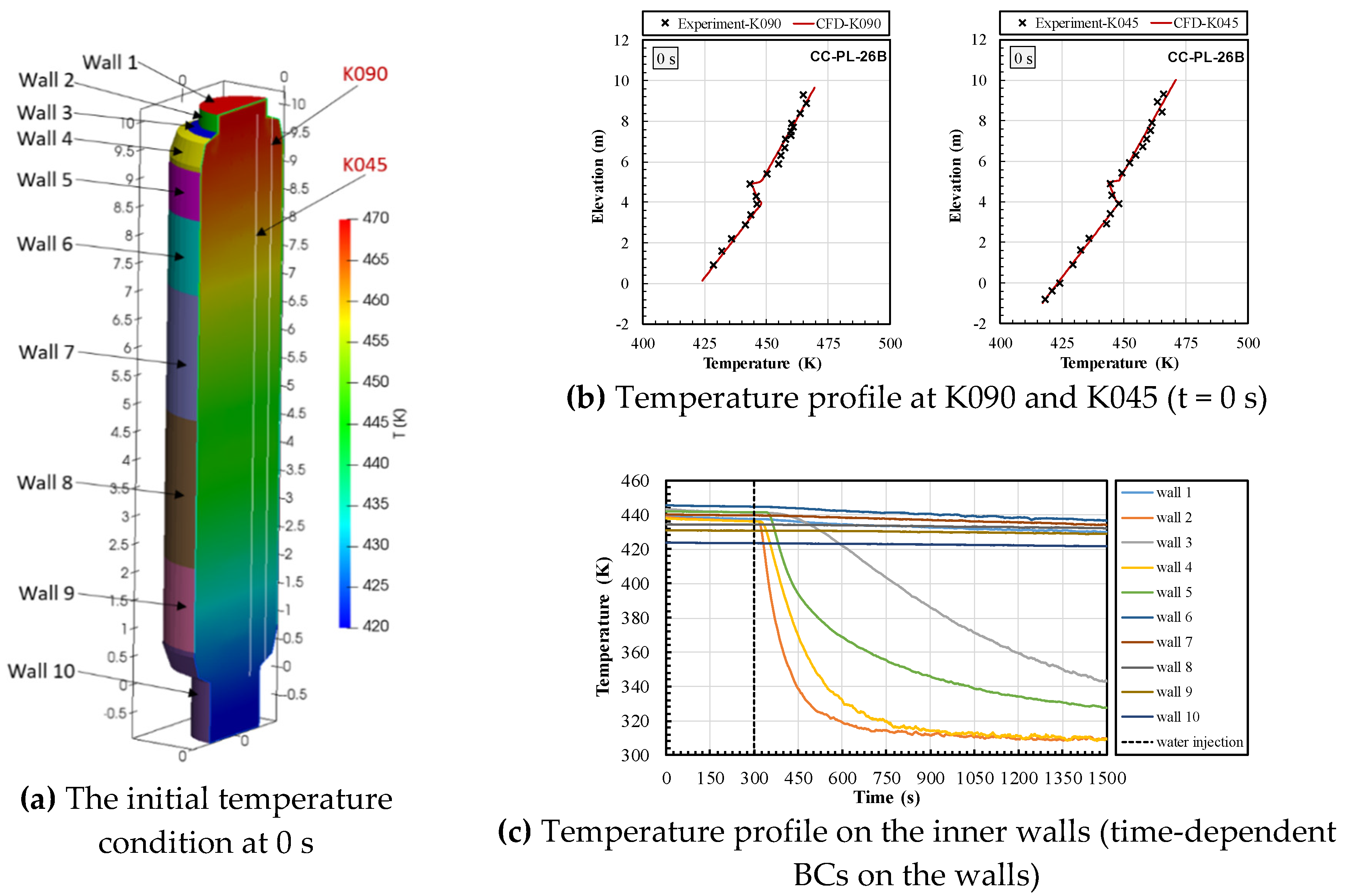
3.3. Initial and Boundary Conditions

3.3.1. Initial and Boundary Conditions Profile

The fluid inside the containment vessel is air, which is treated as an ideal gas. The wall was divided into 10 faces, and it was distinguished by a different color, as shown in Figure 3a. Each face has a time-dependent temperature during the simulation. The temperature value on the walls was obtained from the experimental data of CC-PL-26B, and they were the average temperature of the inner wall vessel, as shown in Figure 3c. In this case, the wall temperatures were modeled as step changes between faces. The wall temperature on each wall was updated every second. It can be observed that the inner wall temperature on the cooled region, i.e., wall2, wall3, wall4, and wall5, decreases rapidly after the water injection. On the other hand, the inner wall temperature on the other walls also decreases gradually but not significant as compared with the cooled region.

The preheating process was done on the test vessel. Thus, the temperature of the flat bar is assumed to be equal with the fluid temperature. The initial temperature of both the fluid and solid regions are given as below:

$${T\left(z\right)|}_{t=0}=\{\begin{array}{c}6.2775\mathrm{z}+423.25\\ -3.4237\mathrm{z}+460.67\\ 4.6436\mathrm{z}+424.51\end{array}\begin{array}{ccc}& & \end{array}\begin{array}{c}if\\ if\\ if\end{array}\begin{array}{cc}& \begin{array}{c}-1\le \mathrm{z}<4\\ 4\le \mathrm{z}<5\\ 5\le \mathrm{z}\end{array}\end{array}.$$

(10)

The above correlations were derived from the experimental results of CC-PL-26B. Figure 3b shows the temperature comparison between the simulation and experimental data on the line K090 and K045.

The summary of the boundary conditions is described in

Table 2. Boundary conditions.

Run ID: CC-PL-26B
Boundary Name	Boundary Condition CHT Model	Boundary Condition Non-CHT Model
Fluid Region
Wall	u = 0, T = Dirichlet (time dependent)	u = 0, T = Dirichlet (time dependent)
Fluid to solid interface	$T_f=T_s$, $-{\kappa }_f\nabla T_f={\kappa }_s\nabla T_s$	none
Solid region
Flat bar ends	$\nabla T=0$	none
Solid to fluid interface	$T_f=T_s$, $-{\kappa }_f\nabla T_f={\kappa }_s\nabla T_s$	none

. Numerical simulation with two different boundary conditions (BCs) was carried out. First, the conjugate heat transfer (CHT) between the solid (flat bars) and the fluid interface was modeled, i.e., CHT model. Second, the solid (flat bars) regions were not modeled, i.e., non-CHT model. The effect of gas radiation heat transfer was not included in the present analysis due to nonparticipating gas (air) being the only fluid inside the containment vessel. However, radiation heat transfer should be included in the model since it has a significant effect on the gas temperature of a humid atmosphere [29] as revealed in the International Standard Problem (ISP-47).

3.3.2. Boundary Conditions—Conjugate Heat Transfer (CHT)

At the interface between solid and fluid regions, an appropriate boundary condition is required to couple the energy equations in both regions. In order to couple heat transfer simulations on their interface, Dirichlet–Neumann coupling was used in the simulation. To derive the equations for this boundary condition, consider the two cells at either side of the interface, such as in Figure 4.

$T_{cf}$ and $T_{cs}$ are the temperature at the cell center of fluid and solid. $T_f$ and $T_s$ are the temperature on the patch for the fluid and solid and $T_{\mathrm{int}}$ is the temperature at the interface. $Q_f$ is the heat flux out of the fluid region and $Q_s$ is the heat flux that enters the solid region. In the Dirichlet–Neumann coupling, the continuity of the temperature and the heat flux on the fluid–solid interface is assumed, therefore:

$$T_f=T_s=T_{\mathrm{int}},$$

(11)

$$-Q_f=Q_s=Q.$$

(12)

From the Fourier’s law, the heat fluxes in the Equation (12) can be calculated as below:

$$-{\kappa }_f\nabla T_f={\kappa }_s\nabla T_s,$$

(13)

where ${\kappa }_f$ and ${\kappa }_s$ are the thermal conductivity of the fluid and solid, respectively.

The temperature gradient at the wall is calculated from the difference between the value at the cell center and wall face divided by the distance between those cell centers:

$$\begin{array}{l}\nabla T_f=\frac{T_{cf}-T_f}{{\delta }_f}={\Delta }_f\left(T_{cf}-T_f\right)\\ \nabla T_s=\frac{T_{cs}-T_s}{{\delta }_s}={\Delta }_s\left(T_{cs}-T_s\right)\end{array}$$

(14)

where ${\Delta }_f=1/{\delta }_f$ and ${\Delta }_s=1/{\delta }_s$. ${\delta }_f$ and ${\delta }_s$ are the distance between the cell centers and wall interfaces of the solid and fluid domain.

Substituting Equation (14) into Equation (13), we get:

$$-{\kappa }_f{\Delta }_f\left(T_{cf}-T_f\right)={\kappa }_s{\Delta }_s\left(T_{cs}-T_s\right).$$

(15)

By simplifying with $T_f=T_s=T_{\mathrm{int}}$, the value of the $T_{\mathrm{int}}$ and $Q$ at the interface can be calculated:

$$\begin{array}{l}-{\kappa }_f{\Delta }_f\left(T_{cf}-T_{\mathrm{int}}\right)={\kappa }_s{\Delta }_s\left(T_{cs}-T_{\mathrm{int}}\right)\\ T_f=T_{cs}\left(\frac{{\kappa }_s{\Delta }_s}{{\kappa }_f{\Delta }_f+{\kappa }_s{\Delta }_s}\right)+T_{cf}\left(\frac{{\kappa }_f{\Delta }_f}{{\kappa }_f{\Delta }_f+{\kappa }_s{\Delta }_s}\right)\end{array}$$

(16)

$$Q={\kappa }_s{\Delta }_s\left(T_{cs}-T_{\mathrm{int}}\right)=-{\kappa }_f{\Delta }_f\left(T_{cf}-T_{\mathrm{int}}\right).$$

(17)

4. Numerical Procedure and the Computational Mesh

An unsteady Reynolds averaged Navier–Stokes (U-RANS) approach was chosen, and the chtMultiRegionFoam solver was used in the simulation. The chtMultiRegionFoam is a solver in OpenFOAM^® for buoyant, turbulent fluid flow, and solid heat conduction with conjugate heat transfer between solid and fluid regions. The gradient terms were discretized by the central differencing scheme, and the divergence terms were discretized by the linear scheme with the total variation diminishing (TVD) scheme. The implicit backward Euler scheme was used for temporal discretization. The coupling between velocity and pressure fields in chtMultiRegionFoam was solved using the PIMPLE algorithm, which is a combination of the PISO (pressure implicit with splitting of operator) and SIMPLE (semi-implicit method for pressure linked equations) algorithms. A standard wall function approach was implemented in the high Reynolds model. Besides, the near-wall region meshes with y + < 1 were constructed to resolve the viscous boundary layer in the low Reynolds model. The time step was adjusted during the transient simulations so that the maximum Courant number was less than 0.5.

Four different computational meshes were constructed to study the effect of grid resolution and near-wall treatment. All meshes for both a high Reynolds number and a low Reynolds number turbulence models were constructed with the hexahedral cells. The grid convergence for a high Reynolds number was ensured by a series of simulations on three different grids. The detail of each grid model is presented in Figure 5 and

Table 3. Computational meshes.

Parameter	Coarse Grid	Medium Grid	Fine Grid	y + = 1 Grid
Number of cells	112,112	373,120	1,026,317	1,847,600
Mean cells size in the bulk region (radial direction)	75 mm	50 mm	35 mm	45 mm
Mean cells size in the bulk region (vertical direction)	75 mm	50 mm	35 mm	50 mm
First cell size	60 mm	50 mm	40 mm	0.5 mm
Mean wall-adjacent cell y+	50	50	50	<1
Near-wall treatment	Standard wall function	Standard wall function	Standard wall function	resolved

.

In the y + = 1 mesh, the typical cell size is 0.5 mm adjacent to the walls and 45 mm × 50 mm in the bulk region. In the coarse, medium, and fine mesh, the typical cell size adjacent to the wall is 60 mm and 50 mm × 40 mm in the bulk region, respectively. The viscous boundary layer near the walls (y + ≤ 1) is resolved in the y + = 1 mesh, and the wall functions were implemented in the near-wall regions of the coarse, medium, and fine grid in order to impose an analytical near-wall solution.

5. Results and Discussions

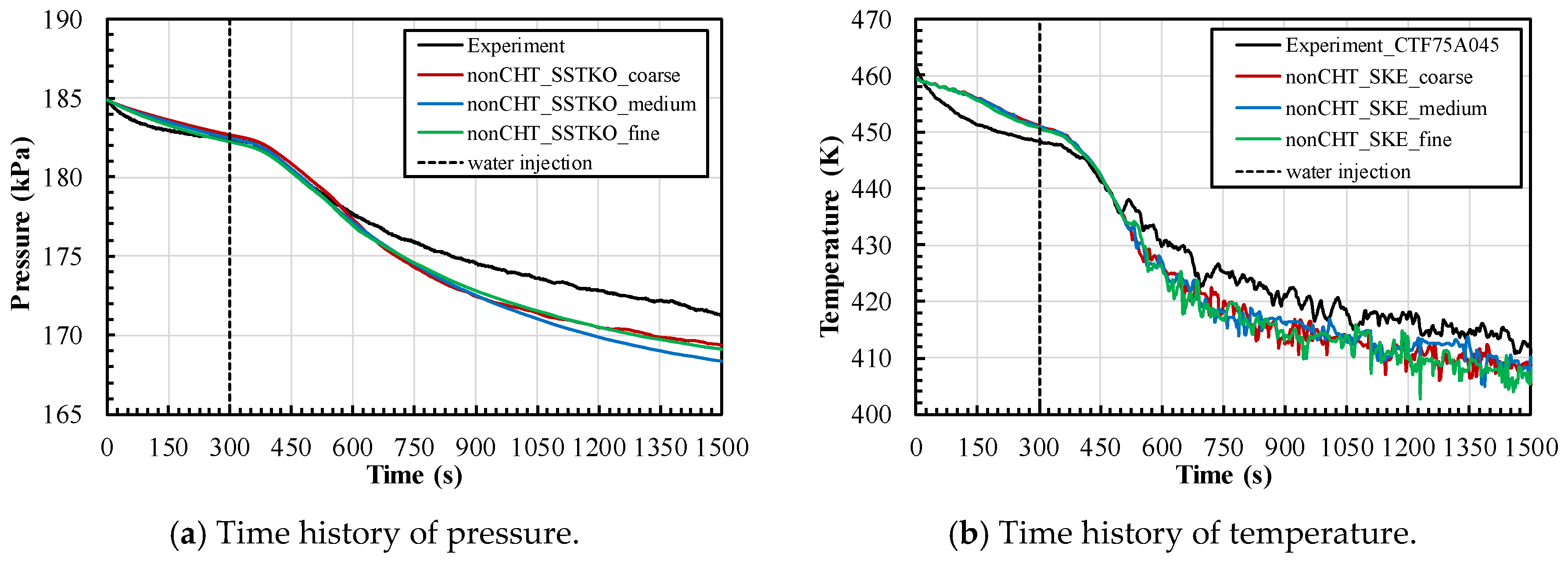
5.1. The Effect of Grid Resolution

The mesh sensitivity study was performed with the standard k-ε turbulence model. Three model domains were tested on CC-PL-26B to study the grid convergence, i.e., coarse, medium, and fine grid. The wall functions were implemented in all model domains. In this grid independency study, the conjugate heat transfer was not modeled. The effect of grid resolution on the pressure and temperature at probe CTF75A045 inside the vessel is depicted in Figure 6. The location of the probe CTF75A045 was located 7500 mm above the bottom vessel and 450 mm away from the vessel wall, see Figure 1a.

The results show that all mesh sizes predict the general trend in both pressure and temperature. The comparison results between the coarse and medium grid show a small discrepancy. The slight difference was also observed on the medium and the fine grid. The discrepancy between the medium and fine grid is less than 1%. It means that a cell size of 50 mm × 50 mm in bulk is sufficient to model the CC-PL-26B test. To reduce numerical cost and also to ensure numerical stability, only the results obtained with the medium grid will be discussed in the next chapters.

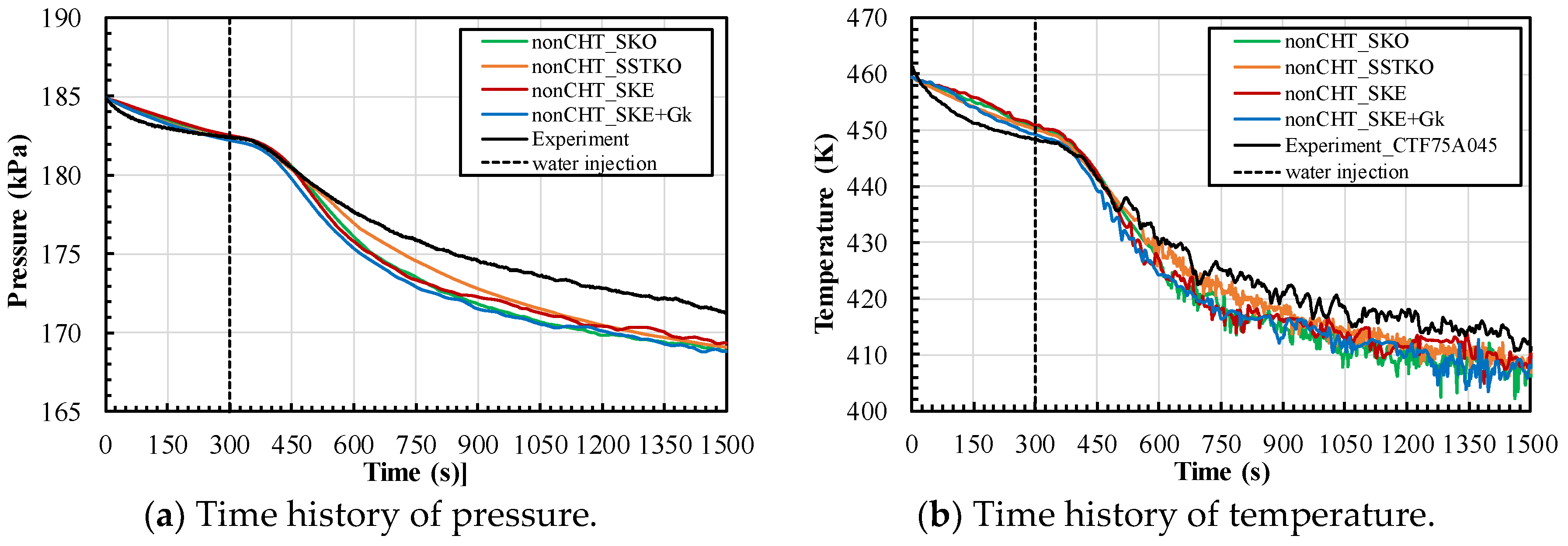
5.2. The Effect of Near-Wall Treatment on Turbulence Model

The results obtained on the medium mesh with wall functions and the y + = 1 grid with the two-layer model are shown in Figure 7. The comparison was performed to assess the effect of near-wall treatment. The standard k-ε turbulence and SST k-ω model were used as a high Reynolds model, and the k-ε Launder–Sharma turbulence model was used as a low Reynolds model. The conjugate heat transfer was not considered in all models.

As shown in Figure 7a, the predicted pressure by means of the high Reynolds model with standard k-ε and k-ω SST (nonCHT_SKE and nonCHT_SSTKO) agrees well, and they are both close to the experimental results, particularly before t = 500 s. The pressure prediction by a low Reynolds k-ε Launder–Sharma model (nonCHT_LS), however, is underestimated, particularly before t = 600 s. It can be observed in Figure 7a that that the standard k-ε turbulence model shows a lower pressure compared with the other models, particularly between t = 500 s and t = 850 s. It might be due to the transition from the laminar natural convection to the turbulent natural convection. As a consequence, the turbulence model with a wall function overestimates the turbulent kinetic energy near the wall since the k-ε turbulence model leads to an overprediction of the turbulent length scale in the flows with adverse pressure gradients, resulting in the overestimation of the heat transfer rates.

Nevertheless, after t = 900 s, the predicted pressure by means of the standard k-ε and k-ω SST turbulence model shows a small discrepancy compared to a low Reynolds k-ε Launder–Sharma model. Their mean deviation is about 0.7%. The predicted pressure and temperature by means of the k-ω SST turbulence model shows a better performance than the standard k-ε turbulence model on the unsteady natural convection inside the large containment vessel.

Figure 7b depicts the time history of the temperature at the probe CTF75A045. The temperature prediction by means of the high Reynolds with the standard k-ε model predicts the general trend but overestimates the heat transfer. Therefore, the predicted temperature is underestimated compared with the experimental data. It can be observed in Figure 8 that both the high Reynolds model and low Reynolds model underestimate the temperature at t = 1500 s. It might be because the internal structure inside the vessel was not completely modeled. It suggests that the effect of the thermal inertia of the internal structure on the overall heat transfer could not be ignored. Hence, it is necessary to model the internal structure of the containment vessel in the CFD simulation. The effect of the internal structure on the overall heat transfer is performed and discussed in Section 5.4.

The implementation of wall functions on the k-ε turbulence model could predict a general trend on both pressure and temperature but are less accurate compared to the experimental results. Results on the k-ω SST turbulence model show a small discrepancy compared with the low Reynolds number Launder–Sharma turbulence model. Thus, it is recommended to resolve the viscous laminar sublayer or choose k-ω SST turbulence models when simulating the natural convection in the large containment vessel, such as the CIGMA facility. In order to reduce the computational cost, the implementation of wall functions on the k-ω SST turbulence model is recommended. In the previous study, the k-ω SST turbulence model is also suggested when validating the CFD model in large containment vessels, such as TOSQAN, THAI, and PANDA [11,29,30]. The effect of the turbulence model is discussed in the next subchapter to confirm and validate the effect of turbulence models on the natural convection in the CIGMA facility.

5.3. The Effect of Buoyancy on the Turbulence Model

The sensitivity study on turbulence models and buoyancy terms in the turbulence model was performed on the medium mesh without the conjugate heat transfer. The turbulence models are listed below:

• nonCHT_SKO: standard k-ω model without a conjugate heat transfer;
• nonCHT_SSTKO: SST k-ω model without a conjugate heat transfer;
• nonCHT_SKE: standard k-ε model without a conjugate heat transfer; and
• nonCHT_SKE+Gk: standard k-ε model without a conjugate heat transfer + buoyancy production in the turbulent kinetic energy.

Figure 9 shows a comparison of the measured and predicted pressure and temperature. The results show that all turbulence models reasonably predict pressure and temperature inside the vessel. However, compared with the experiment, the predicted pressure and temperature are underestimated. The predication of standard k-ω, standard k-ε, and standard k-ε with an additional buoyance term G_k shows a small discrepancy. In the previous study [29,30], the buoyance term G_k had to be included in the turbulence model to predict the erosion of a stratification accurately. As shown in Figure 9a, seemingly, there is no significant effect of the generation of turbulent kinetic energy by buoyancy when the stratification layer is not formed in the initial condition. Thus, the effect of buoyancy on the turbulence generation was small as the difference in density was small.

Table 4. Simulation model deviation from the measurement: effect of turbulence models.

Method	Model	t = 250 s Probe: CTF75A045		t = 750 s Probe: CTF75A045		t = 1250 s Probe: CTF75A045
		Pressure (kPa)	Deviation (%)	Pressure (kPa)	Deviation (%)	Pressure (kPa)	Deviation (%)
Experiment	-	182.570	-	175.88	-	172.56	-
CFD Simulation	SKO	182.787	0.12	173.539	1.33	169.830	1.58
	SSTKO	182.915	0.19	174.272	0.91	170.370	1.27
	SKE	182.831	0.14	173.506	1.35	170.267	1.33
	SKE+Gk	182.508	0.03	172.924	1.68	169.860	1.56

summarizes the absolute deviations between the simulation and experimental results for pressure. The mean deviation of the predicted pressure for all turbulence models at t < 500 s is about 0.2%, and for t > 1000 s is about 2.5%. In between 500 s < t < 1000 s, three turbulence models, i.e., standard k-ω, standard k-ε, and standard k-ε model with additional buoyancy term G_k, the mean deviation is about 1.5%. However, the mean deviation of the SST k-ω model is about 1%. In the present analysis, the SST k-ω model is better than the other turbulence models for predicting the heat transfer on unsteady natural convection inside the large vessel.

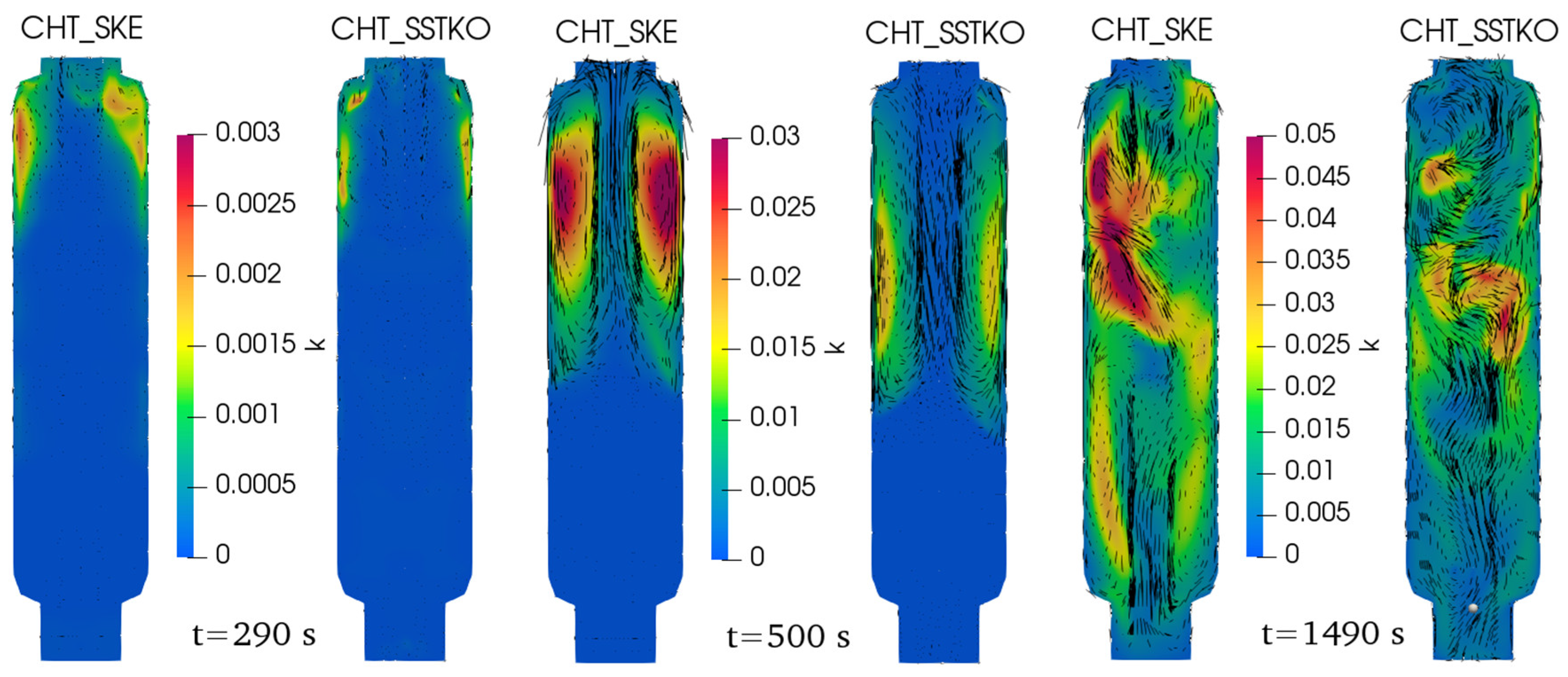
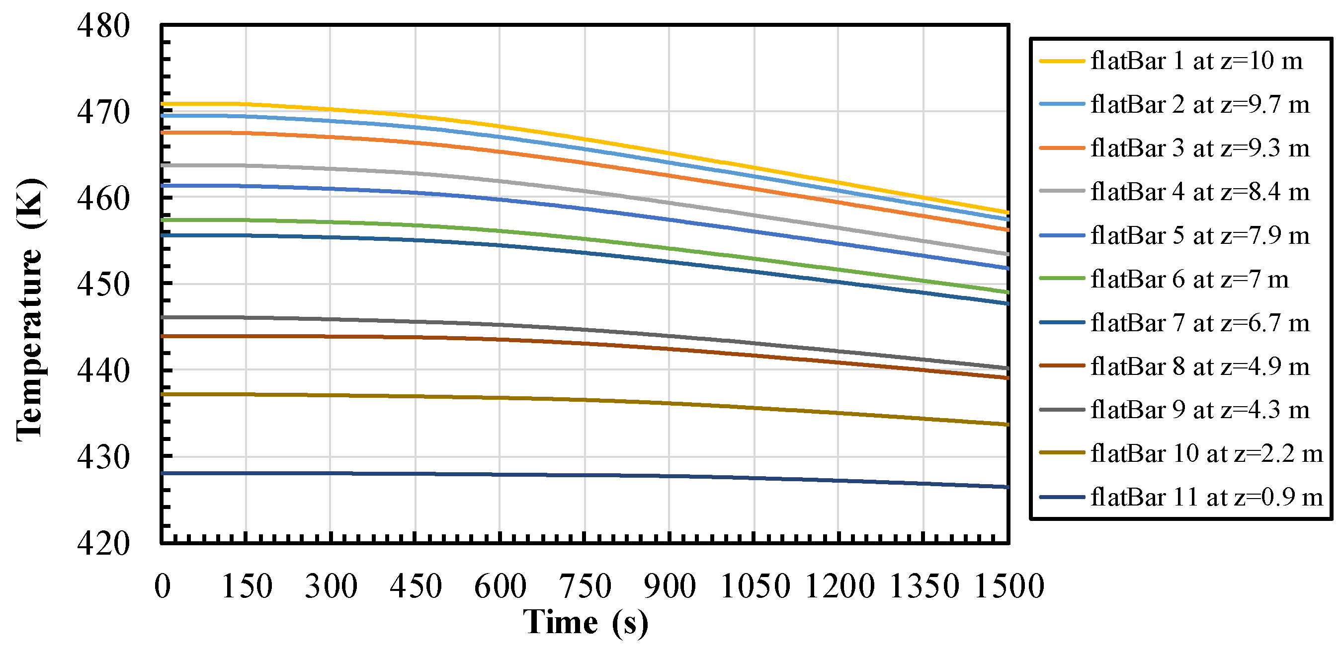
5.4. The Effect of the Solid Region (Flat Bars): Conjugate Heat Transfer Model

As mentioned in Section 5.1, the internal structure might have an influence on the accuracy of the predicted temperature and pressure. In this subchapter, the importance of the internal structure on the heat transfer, i.e., flat bar, is presented and discussed. Two turbulence models were used to investigate the conjugate heat transfer in the CC-PL-26 test. Four different simulations were performed as below:

• CHT_SKE: standard k-ε model with a conjugate heat transfer;
• nonCHT_SKE: standard k-ε model without a conjugate heat transfer;
• CHT_SSTKO: SST k- ω model with a conjugate heat transfer; and
• nonCHT_SSTKO: SST k- ω model without a conjugate heat transfer.

Figure 10 shows the comparison of the measured and predicted pressure and temperature, and

Table 5. Simulation model deviation from the measurement: effect of flat bars.

Method	Model	t = 1500 s Probe: CTF75A045		t = 1500 s Probe: CTF75A045
		Temperature (K)	Deviation (%)	Pressure (kPa)	Deviation (%)
Experiment		411.260		171.270
CFD simulation	nonCHT_SKE	410.140	0.27	169.354	1.18
	CHT_SKE	408.298	0.72	170.150	0.65
	nonCHT_SSTKO	408.511	0.67	169.090	1.27
	CHT_SSTKO	410.569	0.17	170.286	0.57

summarizes the absolute deviations between the simulation and experimental results for temperature and pressure, respectively.

It can be observed that conjugate heat transfer on flat bars has a significant influence on the overall predicted pressure and temperature. Two turbulence models, i.e., standard k-ε and SST k- ω model with a conjugate heat transfer, show a relatively small discrepancy at t = 1500 s, and its mean deviation is about 0.6%. The mean deviation of pressure at t = 1500 s without conjugate heat transfer is approximately 1.2%. In other words, compared with the simulation without a conjugate heat transfer model, the mean deviation of the pressure at t = 1500 s decreases by 0.6% when the heat conduction on the flat bar is taken into account in the simulation. Therefore, the accuracy of the predicted temperature and pressure is improved when the internal structure is considered in the model. A similar tendency is observed in the predicted temperature, as shown in Figure 10b. The predicted temperature increased when the conjugate heat transfer was considered in the model. Temperature fluctuation was observed in the experiment after t = 500 s. All models capture the temperature fluctuation well.

Overall, the SST k-ω model could predict the pressure and temperature inside the vessel well. It seems that the standard k-ε model overestimates the heat transfer rate on the wall. The standard k−ε model is less accurate at predicting the level of turbulent kinetic energy in the stagnation region. Consequently, the heat transfer is also overpredicted in this region [31]. Therefore, the pressure and temperature prediction using the standard k−ε model is underestimated compared with the SST k-ω model. As previously mentioned by Menter [27], mainly, the standard k-ε model tends to overpredict the turbulent length scale in the flows with adverse pressure gradients, e.g., vortex flow. Nevertheless, the predicted temperature and pressure by both the standard k−ε and the SST k-ω model are less than 1%. It can be concluded that the SST k-ω model shows a limited improvement when compared with the standard k-ε model.

Table 6. Computational times.

Model	Computation Times (hour)
CHT_SKE	6.96
nonCHT_SKE	4.12
CHT_SSTKO	5.58
nonCHT_SSTKO	3.51

shows the computational times (wall clock times) for all different schemes. The parallel calculations were performed in the cluster computer using 24 processors. It can be seen in the table that the most time-consuming process is solving the energy equation in the fluid and solid domain (conjugate heat transfer model). Besides, the SST k-ω shows less computational cost compared with the k-ε turbulence model.

Figure 11 shows the snapshots of the predicted turbulent kinetic energy by means of standard k-ε and SST k-ω with a conjugate heat transfer model. These snapshots help to illustrate and understand the flow behavior and its evolution over time inside the vessel. At the beginning (before the water was injected into the upper pool and middle jacket), the predicted turbulent kinetic energy by both models has the same level of magnitude. Its maximum turbulent kinetic energy is about 2 × 10⁻³ m²/s². At t < 300 s, a small discrepancy was observed on both the pressure and temperature for all models.

On the other hand, when the cooling is initiated at the top region of the vessel by water injection, a large temperature gradient increases the heat transfer rate in the cooled wall region. As we can see in Figure 11, at t = 500 s, the natural convection can be noticed by large pair vortex at half of the top vessel and downward flow at the cooled wall region. At t = 500 s, the predicted turbulence kinetic energy employing the standard k-ε model (CHT_SKE) is larger than the SST k-ω model (CHT_SSTKO). It means that the standard k-ε model does not predict the adverse pressure gradient induced by the pair vortex flow well. Otherwise, the SST k-ω model shows significant advantages near the wall.

Finally, at t = 1490 s, the predicted turbulent kinetic energy by both turbulence models has the same level of magnitude. Its maximum turbulent kinetic energy is about 4.5 × 10⁻² m²/s². Furthermore, it can be seen in Figure 11 that the maximum turbulent kinetic energy is not observed adjacent to the wall when the flow becomes unsteady at t = 1490 s. Finally, the large pair vortex flow at the top region of the vessel is no longer observed, and then the large pair vortexes breakdown into smaller vortexes.

5.5. Temperature Profile

The analysis was performed on the SST k-ω model with a conjugate heat transfer (CHT_SSTKO) and a standard k-ε model with conjugate heat transfer (CHT_SKE). The temperature profile in the vertical direction is presented in Figure 12. Figure 12a depicts the vertical temperature on the line K090 before the water is injected into the upper pool and middle jacket. Compared with the experimental data, all turbulence models predict the temperature profile at t = 100, 200, and 300 s well. Figure 12b represents the vertical temperature profile after the water injection. It can be seen, at t = 500 s, that all models could predict the temperature well compared with the experimental data. However, a distinct difference was observed at t = 800 s. At t = 800 s, all models underestimated the temperature profile, particularly the standard k-ε model. The same tendency was also observed at t = 1500 s. Although all models could reasonably predict the temperature profile in the lower cooling region, the large discrepancy was found in the cooling region. All models tended to underestimate the heat transfer rate in the cooling region.

Figure 13 shows the average temperature on the flat bars, which was predicted by employing the SST k-ω model. The temperature on the flat bars at the top of the vessel gradually decreases over time, with no significant decreases at the bottom of the vessel. It indicates that the flat bars contribute to the overall heat transfer inside the vessel.

Overall, the prediction of the temperature profile shows good agreement with the experimental data. Nevertheless, the presence of other modes of heat transfer, i.e., radiation, in the solid region might have a significant influence on the natural convection. If convection is slow, heat radiation may dominate the overall heat transfer. Thus, to assess the containment pressure, consideration of all heat transfer mechanisms in the calculations of temperature is required. It is essential to have a comprehensive investigation of the interaction effects between turbulent natural convection and other modes of heat transfer. Additionally, the influence of the flat bar’s emissivity should be performed. It is important because the flat bars might be oxidized or darkened to result in a high emissivity. Accordingly, the other experiments with its exact distinction from convective heat transfer are required to identify the role of radiation heat transfer as a separate effect in the containment tests used for CFD validation. In this case, the temperature of the flat bar must be measured in order to assess the erroneous predictions due to the absence of the radiation model.

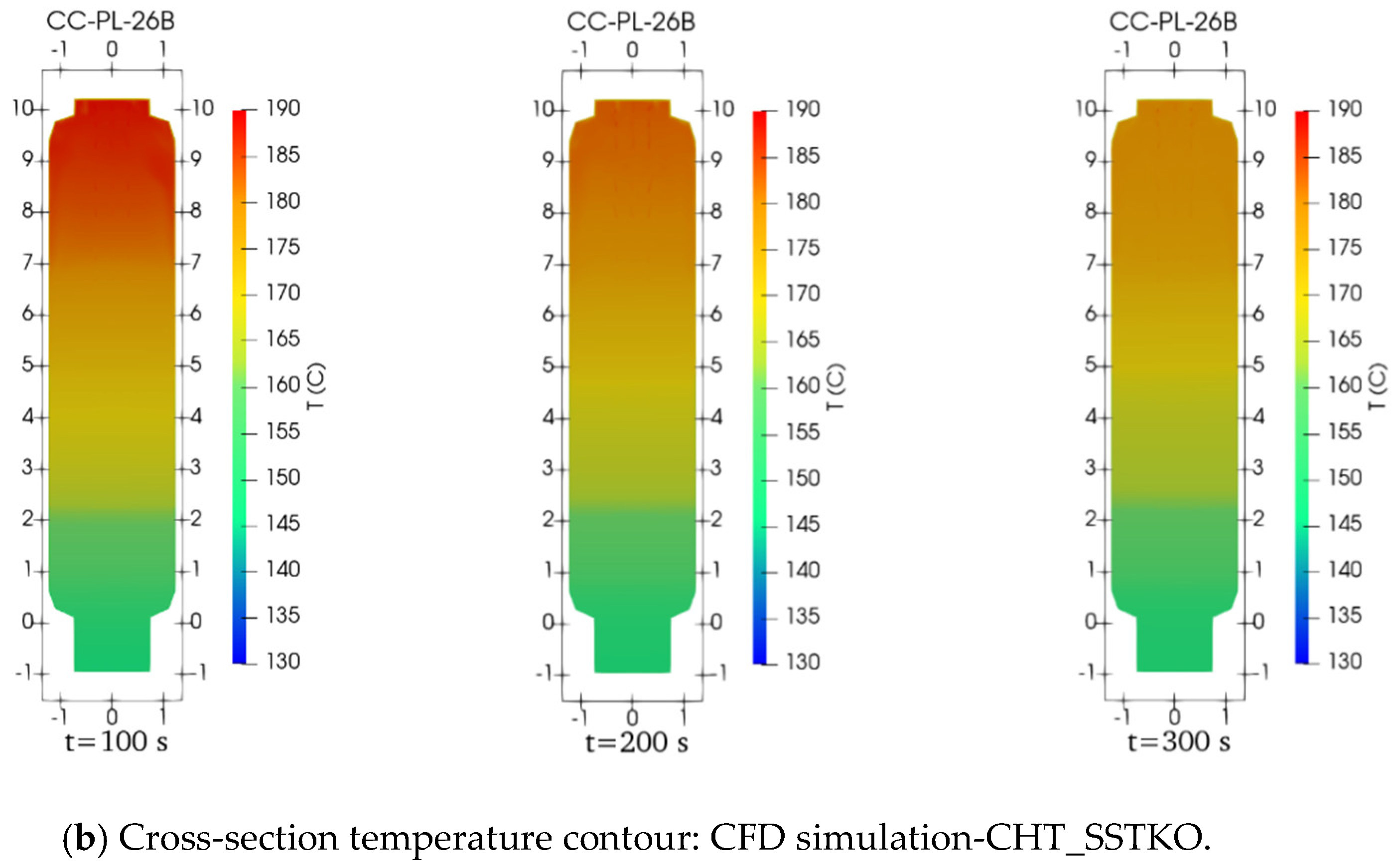
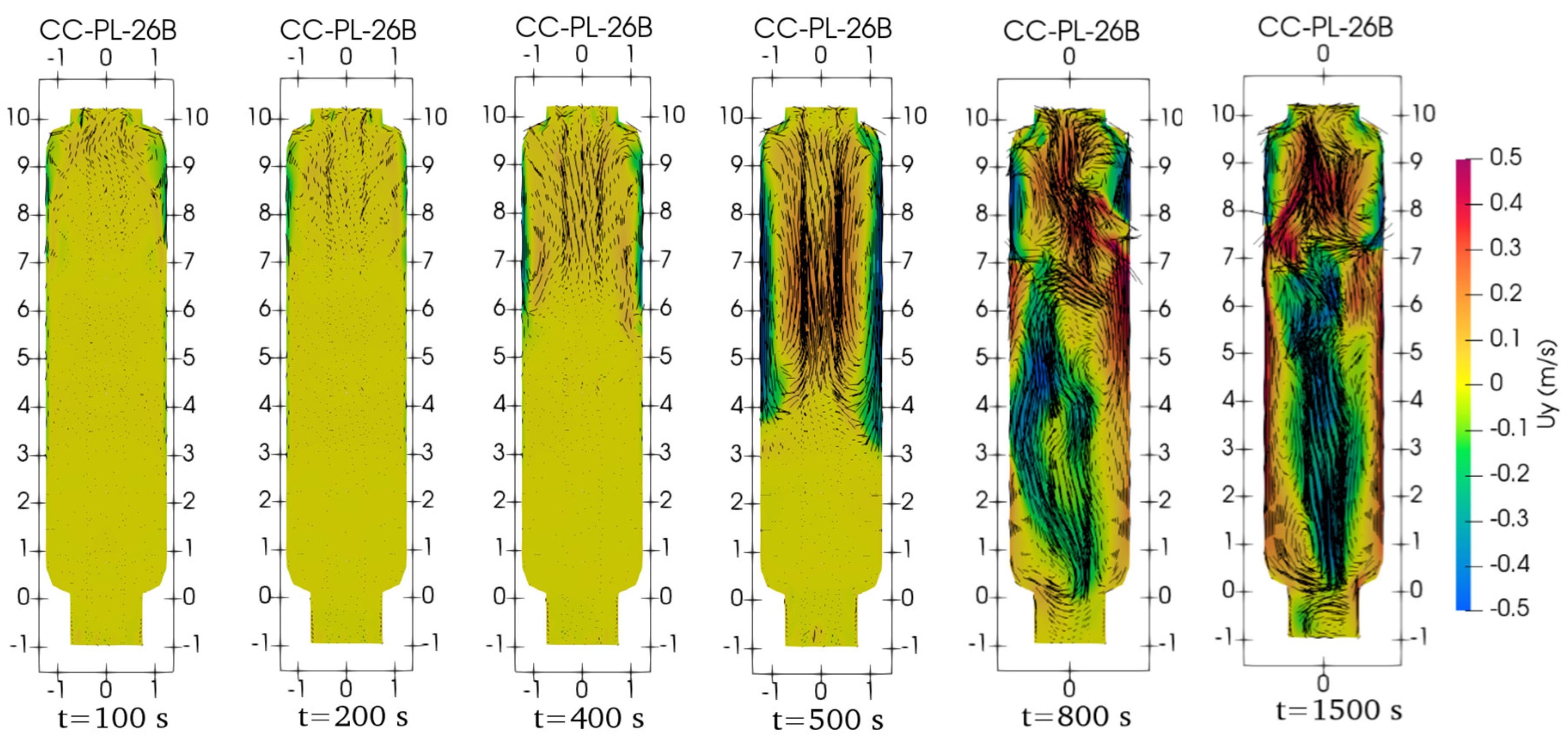
5.6. Contour Plot of Temperature and Velocity

The comparison of the measured and the predicted temperature contour before the water injection is depicted in Figure 14. Figure 14a shows the experimental results. These temperature contours were plotted by a linear interpolation technique. The number of additional points along the x- and z-axis is 10 points. Figure 14b shows the predicted results employing the SST k-ω model. Overall, the simulation results agree well with the measured results. Figure 15 shows the comparison of the measured and predicted temperature contour after the water injection. At t = 500 s, qualitatively, there is no significant difference between the measured and predicted results. However, distinct differences can be observed at t = 800 s and t = 1500 s, particularly at the cooled region of the containment vessel. Nevertheless, the simulation results qualitatively agree with the experimental data and are still reasonable.

Figure 16 shows the predicted vertical velocity inside the containment vessel over a time employing the SST k-ω model. Before the water injection, the downward velocity adjacent to the wall is relatively small compared to the downward velocity at t = 400 s. At t = 500 s, the downward velocity increases in the near-wall region, and the upward velocity increases in the free stream region. As a consequence, a stable pair vortex was observed on the half of the top vessel. Later on, at t = 800 s, the flow becomes unstable, and the pair vortexes breakdown into smaller vortexes. During the simulation, it was observed that the maximum vertical velocity is less than 0.5 m/s.

6. Conclusions

In the present work, the experiment of the natural convection inside the cylindrical containment vessel CIGMA was performed in the CC-PL-26 test. In the test, the outer surface cooling was proposed by injecting the subcooled water into the upper pool and middle jacket. Later on, the unsteady natural convection was analyzed through CFD simulation. The sensitivity analysis, such as the effect of mesh resolution and near-wall treatment, turbulence models, and the conjugate heat transfer, was performed in the numerical simulation. The main conclusions in the present study are summarized as follows:

• External wall cooling is one of the effective alternative ways to remove heat from the containment vessel and mitigate the pressurization. It was observed in the experiment that the pressure and temperature gradually decrease after the water injection into the upper pool and middle jacket.
• The sensitivity analysis by CFD simulation on the mesh resolution suggested that the cell size of 50 mm × 50 mm was sufficient to model the natural convection test in the large cylindrical containment vessel.
• The implementation of the wall function on the high Reynolds number model showed good agreement with the low Reynolds number model.
• The simulation results employing the SST k-ω turbulence model showed better agreement compared with the standard k-ω and standard k-ε turbulence models. Simulations with the Launder–Sharma and SST k-ω turbulence model showed a similar behavior. Besides, the buoyancy effect on the turbulence model did not show a considerable difference in the results when the density difference was small.
• The accuracy of the heat transfer prediction was improved when the solid internal structure inside the containment vessel, i.e., flat bars, was modeled by conjugate heat transfer. It was revealed that the standard k-ε model was overestimated in the turbulent kinetic. Otherwise, the SST k-ω model had better prediction on the vortex flows, leading to improved wall shear stress and heat transfer predictions.
• The heat transfer rate in the cooled region increased gradually with time after the water was injected into the upper pool and middle jacket. Additionally, it was revealed that the standard k-ε model overestimated the heat transfer rate compared with the SST k-ω model.

Overall, the simulation results employing the SST k-ω model with the conjugate heat transfer showed good agreement with the experimental results. The predicted pressure and temperature showed a similar trend with the experimental data. However, a small discrepancy was still observed in the numerical results. It might be due to the uncertainties of the wall temperature in the experiment because the wall on the CIGMA facility, which consists of many flanges. However, the solid flanges were not modeled in the present analysis. Therefore, all solid regions should be modeled to confirm the uncertainty of the wall’s temperature. Furthermore, consideration of all heat transfer mechanisms in calculations of temperature, i.e., conduction, convection, and radiation heat transfer model, will also be assessed in our future work.

References

1. Raj, V.A.A.; Velraj, R. Review on free cooling of buildings using phase change materials. Renew. Sustain. Energy Rev. 2010, 14, 2819–2829. [Google Scholar] [CrossRef]
2. Yeh, L.T. Review of heat transfer technologies in electronic equipment. J. Electron. Pack. Trans. ASME 1995, 117, 333–339. [Google Scholar] [CrossRef]
3. Chan, H.Y.; Riffat, S.B.; Zhu, J. Review of passive solar heating and cooling technologies. Renew. Sustain. Energy Rev. 2010, 14, 781–789. [Google Scholar] [CrossRef]
4. Zvirin, Y. A review of natural circulation loops in pressurized water reactors and other systems. Nucl. Eng. Des. 1982, 67, 203–225. [Google Scholar] [CrossRef]
5. Kim, M.H.; Corradini, M.L. Modeling of condensation heat transfer in a reactor containment. Nucl. Eng. Des. 1990, 118, 193–212. [Google Scholar] [CrossRef]
6. Gupta, S. Experimental investigations relevant for hydrogen and fission product issues raised by the Fukushima accident. Nucl. Eng. Technol. 2015, 47, 11–25. [Google Scholar] [CrossRef] [Green Version]
7. Gupta, S. Thai test facility for experimental research on hydrogen and fission product behaviour in light water reactor containments. Nucl. Eng. Des. 2015, 294, 183–201. [Google Scholar] [CrossRef]
8. Freitag, M.; Schmidt, E.; Gupta, S.; Poss, G. Simulation benchmark based on THAI-experiment on dissolution of a steam stratification by natural convection. Nucl. Eng. Des. 2016, 299, 37–45. [Google Scholar] [CrossRef]
9. Stewering, J.; Schramm, B.; Sonnenkalb, M. Validation of CFD-Codes for Natural Convection and Condensation Phenomena in Containments with German Thai-Experiments, Proceedings of the International Topical Meeting on Nuclear Reactor Thermal Hydraulics (NURETH 2015), Pisa, Italy, 12–17 May 2013; American Nuclear Society: Le Grange Park, IL, USA, 2013; pp. 966–978. [Google Scholar]
10. OECD/SETH-2 Project PANDA and MISTRA Experiments Final Summary Report—Investigation of Key Issues for the Simulation of Thermal-Hydraulic Conditions in Water Reactor Containments; NEA/CSNI/R(2012)5; Organisation for Economic Co-operation and Development/Nuclear Energy Agency Committee on the Safety of Nuclear Installations: Paris, France, 2012.
11. Visser, D.C.; Siccama, N.B.; Jayaraju, S.T.; Komen, E.M.J. Application of a CFD based containment model to different large-scale hydrogen distribution experiments. Nucl. Eng. Des. 2014, 278, 491–502. [Google Scholar] [CrossRef]
12. Zajec, B.; Kljenak, I. Simulation of Natural Circulation Experiment in MISTRA Experimental Containment with OpenFOAM CFD Code. In Proceedings of the International Conference Nuclear Energy for New Europe, Portoroz, Slovenia, 9–12 September 2016; pp. 807.1–807.10. [Google Scholar]
13. Visser, D.C.; Houkema, M.; Siccama, N.B.; Komen, E.M.J. Validation of a FLUENT CFD model for hydrogen distribution in a containment. Nucl. Eng. Des. 2012, 245, 161–171. [Google Scholar] [CrossRef] [Green Version]
14. Robb, K.R. External Cooling of the BWR Mark I and II Drywell Head as a Potential Accident Mitigation Measure–Expanded Scoping Assessment; Oak Ridge National Lab. (ORNL): Oak Ridge, TN, USA, 2018. [Google Scholar] [CrossRef]
15. Gui, M.; Wang, J.; Dailey, R.; Corradini, M.L. Performance Analysis of External Drywell Cooling on BWR Mark II Drywell Head Cavity During a Short-Term Station Blackout Scenario by MELCOR, Proceedings of the International Topical Meeting on Nuclear Reactor Thermal Hydraulics (NURETH 2019), Portland, OR, USA, August 2019; American Nuclear Society: Le Grange Park, IL, USA, 2019; pp. 6418–6429. [Google Scholar]
16. Yonomoto, T. Thermal Hydraulic Safety Research at JAEA after the Fukushima Dai-Ichi Nuclear Power station accident. In Proceedings of the International Topical Meeting on Nuclear Reactor Thermal Hydraulics (NURETH 2015), Pisa, Italy, 12–17 May 2013; American Nuclear Society: Le Grange Park, IL, USA, 2013; pp. 5341–5352. [Google Scholar]
17. Sibamoto, Y.; Ishigaki, M.; Abe, S.; Yonomoto, T. Experimental Study on Outer Surface Cooling of Containment Vessel by Using CIGMA. In Proceedings of the International Topical Meeting on Nuclear Reactor Thermal Hydraulics (NURETH 2017), Xi’an, China, 3–8 September 2017; American Nuclear Society: Le Grange Park, IL, USA, 2017; pp. 1–14. [Google Scholar]
18. Ishigaki, M.; Abe, S.; Sibamoto, Y.; Yonomoto, T. Experiments on Collapse of Density Stratification by Outer Surface Cooling of Containment Vessel: CC-PL-12 and CC-PL-24 Experiments at CIGMA. In Proceedings of the International Topical Meeting on Nuclear Reactor Thermal-Hydraulics, Operation and Safety (NUTHOS-12), Qingdao, China, 14–18 October 2018; pp. 1–11. [Google Scholar]
19. Sibamoto, Y.; Abe, S.; Ishigaki, M.; Yonomoto, T. First Experiments at the CIGMA Facility for Investigations of LWR Containment Thermal Hydraulics. In Proceedings of the International Conference on Nuclear Engineering (ICONE24), Charlotte, NC, USA, 26–30 June 2016; pp. 1–9. [Google Scholar] [CrossRef]
20. Hamdani, A.; Abe, S.; Ishigaki, M.; Sibamoto, Y.; Yonomoto, T. CFD Analysis of the CIGMA Experiments on the Heated Jet Injection into Containment Vessel with External Surface Cooling. In Proceedings of the International Topical Meeting on Nuclear Reactor Thermal Hydraulics (NURETH 2019), Portland, OR, USA, 18–23 August 2019; American Nuclear Society: Le Grange Park, IL, USA, 2019; pp. 5463–5479. [Google Scholar]
21. Bradley, D.; Matthews, K.J. Measurement of high gas temperatures with fine wire thermocouples. J. Mech. Eng. Sci. 1968, 10, 299–305. [Google Scholar] [CrossRef]
22. Hindasageri, V.; Vedula, R.P.; Prabhu, S.V. Thermocouple error correction for measuring the flame temperature with determination of emissivity and heat transfer coefficient. Rev. Sci. Instrum. 2013, 84, 024902. [Google Scholar] [CrossRef] [PubMed]
23. Jones, W.P.; Launder, B.E. The prediction of laminarization with a two-equation model of turbulence. Int. J. Heat Mass Transf. 1972, 15, 301–314. [Google Scholar] [CrossRef]
24. Wilcox, D.C. Turbulence Modeling for CFD.; DCW Industries Inc.: Palm Dr La Canada, CA, USA, 1998. [Google Scholar]
25. Menter, F.R. Two-equation eddy-viscosity turbulence models for engineering applications. AIAA J. 1994, 32, 1598–1605. [Google Scholar] [CrossRef] [Green Version]
26. Launder, B.E.; Sharma, B.I. Application of the energy-dissipation model of turbulence to the calculation of flow near a spinning disc. Lett. Heat Mass Transf. 1974, 1, 131–137. [Google Scholar] [CrossRef]
27. Menter, F.R. Review of the shear-stress transport turbulence model experience from an industrial perspective. Int. J. Comput. Fluid Dyn. 2009, 23, 305–316. [Google Scholar] [CrossRef]
28. Henkes, R.A.W.M.; van Der Vlugt, F.F.; Hoogendoorn, C.J. Natural-convection flow in a square cavity calculated with low-Reynolds-number turbulence models. Int. J. Heat and Mass Transf. 1991, 34, 377–388. [Google Scholar] [CrossRef]
29. Kelm, S.; Müller, H.; Allelein, H.J. A Review of the CFD Modeling Progress Triggered by ISP-47 on Containment Thermal Hydraulics. Nucl. Sci. Eng. 2019, 193, 63–80. [Google Scholar] [CrossRef]
30. Abe, S.; Ishigaki, M.; Sibamoto, Y.; Yonomoto, T. RANS analyses on erosion behavior of density stratification consisted of helium–air mixture gas by a low momentum vertical buoyant jet in the PANDA test facility, the third international benchmark exercise (IBE-3). Nucl. Eng. Des. 2015, 289, 231–239. [Google Scholar] [CrossRef]
31. Craft, T.J.; Graham, L.J.W.; Launder, B.E. Impinging jet studies for turbulence model assessment-II. An examination of the performance of four turbulence models. Int. J. Heat Mass Transf. 1993, 36, 2685–2697. [Google Scholar] [CrossRef]
Figure 1. The schematic drawing of the a Containment InteGral Measurement Apparatus (CIGMA) facility at Japan Atomic Energy Agency (JAEA).
Energies 13 03652 g001
Figure 2. Three-dimensional model geometry and mesh.
Energies 13 03652 g002
Figure 3. Temperature’s initial condition inside the vessel and the boundary conditions at the walls.
Energies 13 03652 g003
Figure 4. Schematic of fluid and solid cell at the interface.
Energies 13 03652 g004
Figure 5. Cross-section view of the four constructed meshes.
Energies 13 03652 g005
Figure 6. Comparison of the measured pressure and temperature (black lines) with the numerical CFD on the coarse mesh (red lines), medium mesh (blue lines), and fine mesh (green lines).
Energies 13 03652 g006
Figure 7. Comparison of the measured pressure and temperature (black lines) with the numerical CFD on the y + = 1 mesh (green line), medium mesh with the standard k-ε turbulence model (red lines), and medium mesh with the SST k-ω turbulence model (blue lines).
Energies 13 03652 g007
Figure 8. Comparison of the measured and numerically predicted temperature profile at K090.
Energies 13 03652 g008
Figure 9. Time history of pressure and temperature as measured (black line) and numerically predicted by means of different turbulence models (colored lines).
Energies 13 03652 g009
Figure 10. Time history of pressure and temperature as measured (black line) and numerically predicted by means of different turbulence models with CHT (solid lines) and without CHT (dash lines).
Energies 13 03652 g010
Figure 11. Comparison of the contour plot of the predicted turbulent kinetic energy, k(m2/s2), by means of different turbulence models.
Energies 13 03652 g011
Figure 12. Influence of the turbulence model with conjugate heat transfer (CHT) on the temperature profile at K090.
Energies 13 03652 g012
Figure 13. The predicted average temperature on the flat bars by means of the SST k-ω turbulence model with CHT.
Energies 13 03652 g013
Figure 14. Comparison of the temperature contour on the cross-section as (a) measured and (b) numerically predicted by means of the SST k-ω turbulence model with CHT before water injection in the upper pool and middle jacket.
Energies 13 03652 g014aEnergies 13 03652 g014b
Figure 15. Comparison of the temperature contour on the cross-section as (a) measured and (b) numerically predicted by means of the SST k-ω turbulence model with CHT after water injection in the upper pool and middle jacket.
Energies 13 03652 g015
Figure 16. The predicted of the vertical velocity (Uy) by means of the SST k-ω turbulence model with CHT.
Energies 13 03652 g016