Abstract
The electromagnetic process happening between an induction brazing coil and the brazing assembly was studied and is described in the following pages. Using the tools of numerical analysis, we managed to achieve 3-D simulation of the process, which includes presentation of the magnetic field, thermal heat transfer, and time dependence. The results presented are considered for two of commonly used materials—copper and stainless steel in the shape of pipes. The induction brazing coil is a complex C-shape to match with the real industrial practices. The results obtained from the model are in accordance with the experimental results, as in both the model and the experiment, the required temperature was reached in about 6 s. It was found that during the brazing process, the inductance of the winding increases by about 4 nH and the resistance by 1.5 mΩ, which is important for the coordination of the power supply.
1. Introduction
The joining of two metal materials by the melting and adding of a filler metal material is known as brazing. The process is performed at temperatures that range from 450 °C to more than 1000 °C depending on the certain case. Achieving such temperatures requires heating technologies like electrical resistive furnaces, gas-flame heated furnaces, or direct torch-flame heating of the brazing area. While the goal is to heat the metal material itself, the use of large heating devices leads to a large loss of energy due to the preheating process. Metals can be heated by technology called induction heating. Any electroconductive material placed in the alternating electromagnetic field becomes heat due to electromagnetic induction phenomena. Using such a technique, while the target materials are electroconductive, the brazing process can be achieved by induction heating. This process is called induction brazing and it was the focus of our work [1,2,3,4].
Brazing is a complex process defined by its physical parameters, such as material properties, process temperatures, time dependence, energy transfer, and technology application. Achieving stable and repeatable results by keeping the quality at high levels is a basic requirement for industrial application. Knowing the influence of each parameter and property gives a strong ability to solve the problem in the best way.
Typical applications of induction brazing are in various industries mostly related with heating, ventilation, and air conditioning (HVAC) systems. Such a process can be successfully used in automotive, home appliances, industrial heating and cooling, and many more areas of the industry manufacture. All these processes are currently performed by highly expensive, energy-consuming, and low-efficiency devices and techniques. Most of them are a difficult subject of automation. The latest achievements in robotics and automation systems correlate well to induction brazing.
The key parameters of the induction brazing process are related with the physics of the materials, their reaction to the electromagnetic energy, and the relation between material properties and the temperature change. To define the process properly, we have to consider the following basic parameters [4,5,6,7]:
- Electrical resistivity—metals with relatively higher values acquire more energy from the field. Different metals also have a completely different temperature relation of this parameter.
- Operating process temperature or brazing temperature—this value is defined by the specifics of the joined metals and the brazing alloy used. Usually, this point or area is specified by the process engineers designing the process.
- Time for brazing—the requested time is usually as short as possible. However, this also has a process time for alloy flow between the two metals. So, fast heating is just one side of the coin, while achieving brazing is the other. Usually, the temperature of the joint area has to be kept in a certain range for a certain amount of time to ensure good flow of the brazing alloy.
- Size of the joined pieces or size of the brazing zone—pipe sizes that have been brazed can vary from less than 1 mm to up to 50 mm or even more. The problem with bigger sizes is the provision of relatively equal heating to the whole of the joint. Occasionally, brazing can be made in steps from two or even more sides (directions).
- Shape of the assembly—sometimes, the brazing area is not fully directly accessible. This is a source of challenges to define and achieve the proper process, by just performing experiments or tests.
Finding a technical solution of the induction brazing can be done by two main approaches:
- Laboratory experiments and industrial test—this approach gives good results and definitely provides experience and data for post-process analysis. The problem is that the complex shapes of the coils and the joint assemblies require time for engineering and manufacturing of complex tools to perform the test. Each new iteration starts from the beginning.
- Advanced method with combination of real test data and numerical analysis—a strong instrument adds efficiency and effectiveness to the final technical solution. Nowadays, the use of computer hardware and software tools provides a different view over this complex process.
Numerical analysis or just simulation is an engineering application of scientific methods extracted from physics, mathematics, chemistry, and computer technology. Processes like brazing may look simple the first time, but combined with an electromagnetic field, it can become real complex. The aim when performing simulation of some set items and their environment is to simplify the shapes and volumes as much as possible. This makes the task more achievable. For example, if there is an axial symmetry, then 2-D analysis can be easily used. It is less time consuming due to its quick setup and computational time, which is often in a few seconds. On the other hand, 3-D analysis requires more time and resources dedicated to it. Solutions are complex and reaching them is not an easy job. Do we really need to perform such a complex analysis to obtain our goals? The answer to this question comes up by trying to realize the volume of the simple task—the complex shape of the coil, electromagnetic field distribution, current density distribution, resultant heat sources, and some process properties like proper coil cooling.
The common case for induction brazing is to join two pipes of a similar size made of the same or different metal materials. The filler material is also an alloy of several compositions mostly on a metal base. The problem here is how to generate a proper electromagnetic field around the joining area. The use of a simple helical coil is not applicable in many cases because the pipes are part of an assembly or even of a whole device. The only option left is to access the joint from one of the sides. This raises the need of more complex coils to be put on a service.
Modeling is based on a real brazing system with a C-shape coil. The complex design of the coil provides a non-symmetric distribution of the electromagnetic field and the resulting heating pattern. This appears to be a rarely studied matter, with special attention paid to the parameter dependence of the induction coil, which is important for induction power generator load matching.
To simulate the brazing process, we need several inputs as the basis of our task:
- A 3-D model of the complex coil—it can be constructed by using of a software designing tool like ®Solid Works.
- Some experimental data about the electromagnetic field operating frequency, coil excitation currents, and expected process time—data taken from application test reports provided by ©Ultraflex Power Technologies application Lab [4].
- Geometry of the brazing assembly, its size, and materials.
- Software tool that is capable of performing complex 3-D numerical analysis—®COMSOL Multiphysics.
- Hardware platform to perform this heavy task.
For the presented application of induction brazing, no studies have been performed related to 3-D modeling of an asymmetric inductor and on this basis to obtain the dependences of the change of R and L during the technological process. Determining the power losses that are related to the cooling of the inductor and the total power required are also included. All these parameters defined by us are basic for the design of power electronic devices that generate the necessary high-frequency energy.
The paper is organized into the following sections:
- Description—details of the study inputs combined with the theoretical fundamentals included as methods and approaches.
- Validation of the model—basic comparison with other analytical methods (theory and practice) to prove our model’s validity.
- Results—detailed results representation of the simulation outputs and exports.
- Coil analysis—in this section, results for the changes of the coil inductance and resistance with the time are presented.
2. Description
The equations describing the brazing process, or more generally, the processes in induction heating systems, are well known (see, e.g., [1,2]). Additionally, the numerical methods for their solution were developed years ago. Initially, many authors used relatively simple own codes for their models. This approach was successful in 1-D and 2-D models and lead to many important results being obtained that explain the basic features of the studied systems. At the same time, the simplifications in these models do not permit their application for obtaining the parameters of real systems. The next step—realistic 3-D modelling of existing systems—requires the use of commercial software like Comsol Multiphysics. Of course, the software package is only an instrument for the modelling of systems with a complicated geometry and cannot take the role of the author in the choice of the processes into account, as well as the studied parameters and in the interpretation of the results.
We decided to describe the brazing process with the parameters and aspects vital for its industrial application. Modeling activities are processed by defining the following inputs [7,8,9,10,11,12,13,14]:
Model geometry (Figure 1):
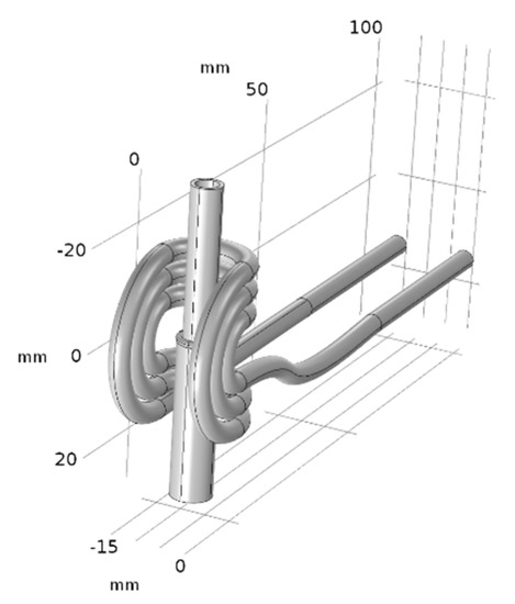
Figure 1.
Model geometry.
- o
- C-shape brazing coil for small tube diameters up to 10 mm.
- o
- Brazing assembly consisting of pipes—8 × 1 mm and 6 × 0.75 mm.
- o
- Brazing alloy—preformed ring—6 × 0.6 mm.
- o
- Surrounding area—block 200 × 200 × 220 mm.
Materials:
- o
- Coil—copper pipe 4 × 0.5 mm.
- o
- Brazing assembly pipes—simulation performed for two cases: Copper and stainless steel AISI 316.
- o
- Brazing alloy—copper to copper pipes—copper (similar to CuP7). Steel to steel—silver (similar to high silver brazing alloys).
The electrical conductivity of the material σ is given by its temperature dependence (Linearized resistivity):
where:
- ρ0—reference resistivity, Ω.m;
- α—resistivity temperature coefficient, n/a; and
- Tref—reference temperature, °C.
Coil excitation can be defined in several ways depending on the goals of the simulation requirements. This part also defines the energy source of the system. In our case, the induction brazing system power source consists of a Radio Frequency (RF) generator, a matching circuit station and remote inductor station, know more as a brazing gun. All these parts of the system are suitable to be presented as a current source while during real operation, control is applied to the RF generator output current. For both brazing cases simulated, copper to copper and steel to steel, we used the following parameters (Table 1).

Table 1.
Main simulation parameters.
The electrical parameters of the simulation were based on real laboratory data experiments and industrial trials.
The complex heat transfer solution for the heated parts (brazing joint and coil) is presented by (2):
where:
- md—material solid density, kg/m3;
- C—material solid heat capacity at constant pressure, J/(kgK);
- k—material solid thermal conductivity, W/(mK); and
- Q—heat source, W/m3.
In the term of the heat source:
where E is the induced electric field intensity.
Energy losses related to the brazing assembly during the heating process can be summarized in two ways: Convection heat flux—energy lost in surrounding air heating—and radiative heat flux.
The boundary conditions on the surface of the coil and of the workpiece are for normal energy flux determined by convection and radiation:
where:
- h—heat transfer coefficient;
- ε—surface emissivity;
- σ—Stefan–Boltzmann constant; and
- Tamb—ambient temperature (surrounding air in our case).
In addition, the coil is cooled by water flowing in an internal cooling channel. Following [11], the water cooling is presented as an additional (negative) heat source:
where:
- mt—the water mass flow, kg/s;
- Tw—water inlet temperature; and
- V—the volume of the water inside the coil.
Geometry meshing as a vital part of the simulation process is presented in Figure 2. Considering a phenomenon like the skin effect and proximity effect, some special attention was focused over the elements of the mesh related to both electroconductive pars—the coil and brazing assembly.
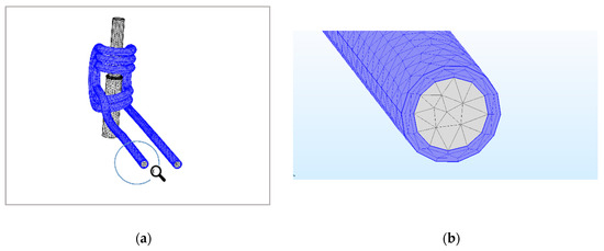
Figure 2.
Model mesh (a), Coil mesh (b)
3. Validation of the Model
The shape of the coil is complicated, and its inductance cannot be calculated analytically. In order to check the reliability of the obtained results, they were compared with results for axisymmetric coils with a similar size and five windings. First, the analytical formula (6):
was applied for a coil with N = 5, length l = 20 mm, and radius R = 8 mm. The result is inductance of the coil L = 3.15827 × 10⁻⁷ H and resistance R = 0.0013 Ohm (ρ—specific electrical resistivity, S—cross section of the coil conductor). The analytical Formula (6) is valid for an infinite coil and it overestimates the inductance value. The next step is a 2-D axis-symmetric numerical model for a coil with the same parameters. The finite length of the coil leads to a decrease of the inductance to L = 2.2131×10⁻⁷ H while the value of the resistance is the same (R = 0.0013 Ohm). These results were obtained at low frequency. Increasing the frequency to 100 kHz (in the range of operation of the real brazing system) leads to an increase of the resistance to R = 0.0048 Ohm because of the skin effect. In addition, a 3-D model of a helical coil also taking into account the leads was developed. The value of the inductance is in the same range like in the previous cases (L = 2.9154 × 10⁻⁷ H) and because of the increased length of the conductor, the resistance is higher, changing from 0.0018 Ohm at low frequencies to 0.0074 Ohm at 100 kHz.
The inductance and the resistance from the model of the brazing system without a workpiece are 2.82 × 10⁻⁷ H and 0.0066 Ohm, respectively. Therefore, the results from the model of the brazing system are in the expected limits.
Experimental results taken from the application test records provided by UltraFlex Power Technologies are presented at Table 2. Tests were performed by the use of its handheld induction brazing system UBraze [15].
Table 2.
Laboratory test results reference.
It can be noted that the two experiments were performed by using two different coil configurations—three turns for copper and one turn for stainless steel. In order to better match to our model, we decided to decrease the coil current for the steel-to-steel study while our coil had three turns for both cases [16,17,18].
4. Results
Obtaining useful results for understanding the brazing process was the main goal of this work. Visualization of the invisible physical phenomena and its time dependence is one of the main advantages of our approach. Such a technique gives us a strong instrument for detailed analysis of the usually hidden aspects of the complex relationship between electromagnetism and heat transfer. Using it for analysis of an industrial process like brazing can optimize more of its parameters and significantly improve the performance [18,19,20].
One of the most interesting results of the simulation model is the magnetic flux density distribution across the 3-D space. As it can be expected, there are areas with more concentrated magnetic flux because of the complex coil shape. The 2-D cross-section views are presented in Figure 3. While the magnetic flux is a vector, its direction in a particular moment of time can also be visualized (Figure 4).
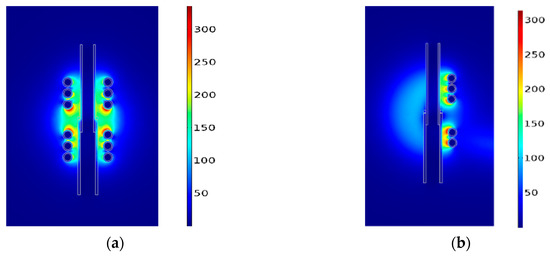
Figure 3.
Magnetic flux density—coil and brazing assembly, Bm, (mT), (a) front view, (b) side view.
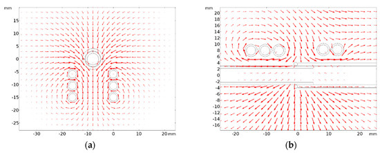
Figure 4.
Magnetic flux vector—coil and brazing assembly, (a) top view, (b) side view.
The electric current is one of the key parameters of the whole process. Its surface density distribution is visualized on Figure 5. Looking at the coil Figure 5b, it is easy to observe the proximity effect of the high frequency electrical current flowing though the coil conductor. The C-shape of the coil defines this complex pattern. From a practical point of view, regions with higher current density can cause potential local overheating. This information can be used for fine adjustment of the coil shape [20,21,22].
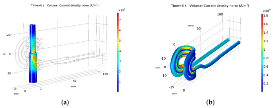
Figure 5.
Current density (copper), (a) brazing assembly, (b) coil.
Magnetic flux causes a “footprint” of electric current density over the brazing assembly presented on Figure 5a. It can be directly related to the resulting heat source (Figure 6a).
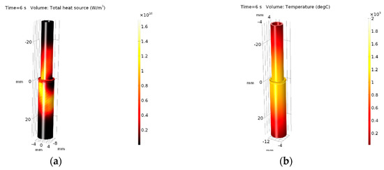
Figure 6.
Heating—brazing assembly (copper), (a) heat source, (b) temperature distribution after 6 s.
The final resulting heating of the brazing assembly is one that can be observed during real laboratory or industrial tests. However, it is not so easy to be analyzed or even measured as the process times are relatively short. The simulation approach allows more detailed study and estimation at any moment. Figure 6b presents the temperature distribution over the brazing assembly after 6 s of heating. It matches very well to the test results.
The results for the more detailed analysis about our case are presented in the following figures. Using the simulation, we managed to compare two cases common for the industrial practice—brazing of copper-to-copper pipes and brazing of stainless-steel pipes.
Brazing of these two cases requires similar temperatures to be reached in order to melt the brazing alloy ring and provide good flow into the gap between the pipes. Copper pipes are brazed by using an alloy with a melting temperature in the range of 640–720 °C. The requested temperature into the brazing area is around 800 °C. Figure 7a shows that this value was achieved at around 3.5 s after the start. At this point, it is reasonable to slow down the heating (by lowering the power) and try to keep the temperature in the requested range for 2 or 3 s to provide complete melting and flow of the alloy. Stainless-steel pipes are brazed by using an alloy with a temperature range of 780–840 °C. The operating temperature here is around 900 °C. From Figure 7b, we can note that this happens 4.5 s after the start. Again, the temperature has to be kept for 2–3 s. These two figures give us a moment of time when we have to start maintaining the temperatures.

Figure 7.
Heating—brazing assembly, (a) copper, (b) stainless steel.
The acquisition of power from the magnetic field is strongly affected by the material properties. As it is presented in Figure 8, it is also time dependent as the temperature significantly changes during the heating. The performance of the two materials is different and it needs to be taken into consideration. Here, it is the main difference between induction heated brazing and the other contact or convection methods. The magnetic field needs to have enough power to provide stable and reliable heating. From these figures, we can estimate the required power needed to be transferred to the brazing assemblies. The main difference about the power required for the brazing of each material is caused by their electrical conductivity and temperature dependence of this parameter.
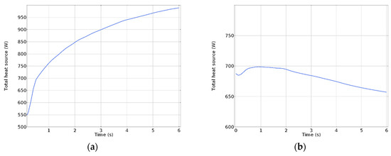
Figure 8.
Heating power—brazing assembly, (a) copper, (b) stainless steel.
The next two figures (Figure 9a,b) are the essential estimation of the induction brazing system. Here, we can see the required electrical power that needs to be applied to the induction coil in both cases of brazing. As expected, it is quite different: Copper requires significantly more power than stainless steel. This is mostly caused by the different coil current excitation. A similar heating effect for both materials is achieved by using significantly different coil currents—copper is heated by the use of 700 A, while for the stainless steel, we used 350 A.
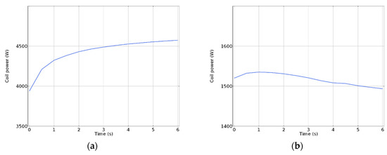
Figure 9.
Coil power, (a) copper, (b) stainless steel.
The heat power losses are presented in Figure 10. Only the copper-to-copper case is visualized for reference. It can be estimated that the sum of the heating losses is a significant part of the transferred energy, at around 20%.
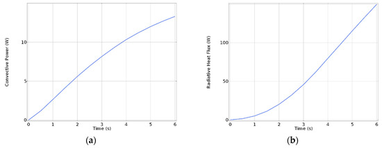
Figure 10.
Power loss—brazing assembly (copper), (a) convection, (b) radiative.
At the end, a heat loss dissipated into the induction coil is shown in Figure 11. Again, only the copper-to-copper case is presented. This estimation is important for induction cooling system evaluation.
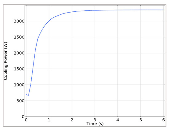
Figure 11.
Cooling power—coil (copper).
5. Coil Analysis
In this section, the results for the changes of the coil inductance and resistance with time are presented.
The coil and the workpiece could be presented as a transformer, where the workpiece plays the role of a one turn secondary coil (Figure 12). Eg is the electromotive force (EMF) of the generator (more precisely, this is the voltage at the ends of the coil), R1 and L1 are the resistance and the inductance of the coil, and R2 and L2 are the resistance and the inductance of the workpiece, respectively.
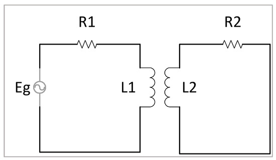
Figure 12.
Transformer presentation of the coil and of the workpiece.
Assuming time dependence of the currents and voltages are of the type exp(jωt), from Kirchhoff’s second law, we obtain:
where I1 and I2 are the currents in the coil and in the workpiece, and E12 and E21 are the induced EMFs:
where M is a mutual inductance.
Expressing I2 from (8):
The equation for Eg is obtained in the form of:
From (10), the resistance and the inductance of the system are:
with:
Therefore, introducing the workpiece into the coil leads to an increase of its resistance and decrease of its inductance.
The time dependence of the resistance and of the inductance of the system (Figure 4) is determined by the dependence of the material conductivity with respect to the temperature. Because of the water cooling, the increase of R1 with time is relatively weak. The behavior of ΔR is more complicated (12). At R2 = 0 and R2 = ∞, its value is zero. The maximum of ΔR is at R2 = ωL2. At the conditions of our model, 0 < R2 < ωL2 and ΔR increases with the resistance R2 (Figure 5).
With the temperature increases and the conductivity decreases, the skin depth in the coil and in the workpiece increases and the electric current penetrates deeper in the metal. For the coil, this means an increase of its cross section and a relatively small increase of the inductance L1 (Figure 13). In opposite, for the workpiece, the effective radius becomes smaller and L2 decreases. In combination with the decrease of the mutual inductance and increase of R2, this leads to lower ΔL (Figure 14) and a rise of L (Figure 13) with the temperature.
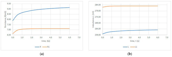
Figure 13.
Resistance (a) and inductance (b) of the system with (blue lines) and without (red lines) a workpiece as a function of time.
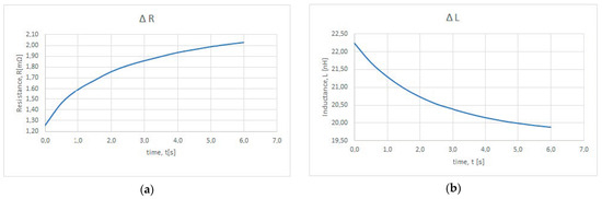
Figure 14.
ΔR (a) and ΔL (b) as a function of time.
The changes of the coil parameters during the brazing process are of significant practical interest as they affect the matching of the generator and the coil and the effectiveness of the power transfer.
6. Conclusions
There are FEM brazing models, but they are usually on axial-symmetric coils. We presented that this modeling method can also be used for windings with a more complex shape. We presented, for the first time, the change of the parameters of the winding during the process (inductance and resistance) as well as brazing of different materials. These results are important for determining the parameters in the design of the power electronic converter. The main goal was to realize different combinations of brazing materials with one converter. Modeling helped us determine the limits of change in the power and frequency so that we could design the converter.
During our study, we managed to achieve a successful 3-D simulation of the induction brazing process. Graphical and numerical representation of the key parameters and their time dependence provided a better look over the complex relation between the electromagnetic field and the resulting material heating. Estimation of the required electrical power directly refers to the design consideration of the induction brazing system. Complex coil design was estimated, and the further analysis and optimizations were possible based on the presented modeling. Power heat losses were estimated and visualized for both main components of the brazing assembly with its convection and radiation emissions and the induction coil with the heat dissipated into the cooling water.
The presented approach and the obtained results can be useful for application and process development engineers in the area of industrial manufacturing. Using the tools of the simulation, induction brazing system components can be evaluated in detail. The model adds abilities to solve practical problems, such as:
- Coil shape and size estimation and basic optimization;
- Power estimation of induction generator;
- Process time calculation; and
- Cooling system power and size estimation.
Author Contributions
D.G., K.T. and N.H. were involved in the full process of producing this paper including conceptualization, methodology, modelling, validation, visualization, and preparing the manuscript. All authors have read and agreed to the published version of the manuscript.
Funding
This research was funded by the European Regional Development Fund within the Operational Program “Science and Education for Smart Growth 2014–2020” under the Project CoE “National center of mechatronics and clean technologies “BG05M2OP001-1.001-0008”.
Conflicts of Interest
The authors declare no conflict of interest.
References
- Roberts, P.M. Introduction to Brazing Technology; CRC © by Taylor & Francis Group, LLC: New York, NY, USA, 2016; ISBN 978-1-4987-5845-1/1498758452. [Google Scholar]
- Rudnev, V.; Loveless, D.; Cook, R. Handbook of Induction Heating, 2nd ed.; CRC Press: New York, NY, USA, 2017; ISBN 978-1-1387-4874-3/1138748749/978-1-4665-5395-8. [Google Scholar]
- Fabian, R. (Ed.) Vacuum Technology: Practical Heat Treating and Brazing; ASM International: Cleveland, OH, USA; ISBN 0-87170-477-3/9781615031511/1615031510/9780871704771.
- Wei, S. Research trends in brazing and soldering. Weld. Tech. Rev. 2017, 89. [Google Scholar] [CrossRef]
- Theodoulidis, T.P.; Tsiboukis, T.D.; Kriezis, E.E. Analytical solutions in eddy current testing of layered metals with continuous conductivity profiles. IEEE Trans. Magn. 1995, 31, 2254–2260. [Google Scholar] [CrossRef]
- Zhang, J.; Yuan, M.; Xu, Z.; Kim, H.J.; Song, S.J. Analytical approaches to eddy current nondestructive evaluation for stratified conductive structures. J. Mech. Sci. Tech. 2015, 29, 4159–4165. [Google Scholar] [CrossRef]
- Khazaal, M.H.; Abdulbaqi, I.M.; Thejel, R.H. Modeling, Design and Nalysis of an Induction Heating Coil for Brazing Process Using FEM. In Proceedings of the Al-Sadeq International Conference on Multidisciplinary in IT and Communication Science and Applications (AIC-MITCSA), Baghdad, Iraq, 9–10 May 2016; pp. 1–6. [Google Scholar] [CrossRef]
- Stennikov, V.N. The Scientific Development of Brazing Technology Electronic Devices. In Proceedings of the 13th International Scientific-Technical Conference on Actual Problems of Electronics Instrument Engineering (APEIE), Novosibirsk, Russia, 3–6 October 2016; pp. 121–122. [Google Scholar] [CrossRef]
- Ahn, S.H.; Hong, J.; Joung, C.Y.; Heo, S.H.; Yang, T.H.; Jang, S.Y. A Study on Temperature Control of Induction Brazing Coil. In Proceedings of the 15th International Conference on Control, Automation and Systems (ICCAS), Busan, Korea, 13–16 October 2015; pp. 2080–2082. [Google Scholar] [CrossRef]
- Shuzu, Z.; Gewen, K. Research on Intelligent Control Strategy of Temperature System of Industrial Brazing Furnace. In Proceedings of the IEEE 2011 10th International Conference on Electronic Measurement & Instruments, Chengdu, China, 16–19 August 2011; pp. 65–67. [Google Scholar] [CrossRef]
- © COMSOL. Single-Turn and Multi-Turn Coil Domains in 3D, 2012.
- Aranaga, S.; Izcara, J.; del Río, L.; Vallejo, H.; Seco, M. Thermal Modelling of a Brazing Process of Vacuum Interrupters. In Proceedings of the 27th International Symposium on Discharges and Electrical Insulation in Vacuum (ISDEIV), Suzhou, China, 18–23 September 2016; pp. 1–4. [Google Scholar] [CrossRef]
- Pánek, D.; Orosz, T.; Kropík, P.; Karban, P.; Doležel, I. Reduced-Order Model Based Temperature Control of Induction Brazing Process. In Proceedings of the Electric Power Quality and Supply Reliability Conference (PQ) & 2019 Symposium on Electrical Engineering and Mechatronics (SEEM), Kärdla, Estonia, 12–15 June 2019; pp. 1–4. [Google Scholar] [CrossRef]
- Pánek, D.; Karban, P.; Doležel, I. Calibration of numerical model of magnetic induction brazing. IEEE Trans. Magn. 2019, 55, 1–4. [Google Scholar] [CrossRef]
- UltraFlex Power Technologies. 2020. Available online: https://ultraflexpower.com/ (accessed on 10 January 2020).
- Chabodez, C.; Clain, S.; Glardon, R.; Mari, D.D.; Rappaz, J.; Swierkosz, M. Numerical modeling in induction heating for axisymmetric geometries. IEEE Trans. Magn. 1997, 33, 739745. [Google Scholar]
- Leitner, M.; Aigner, R.; Grün, F. Numerical fatigue analysis of induction-hardened and mechanically post-treated steel components. Machines 2019, 7, 1. [Google Scholar] [CrossRef]
- Dong, H.; Zhao, Y.; Yuan, H. Effect of coil width on deformed shape and processing efficiency during ship hull forming by induction heating. Appl. Sci. 2018, 8, 1585. [Google Scholar] [CrossRef]
- Naar, R.; Bay, F. Numerical optimisation for induction heat treatment processes. Appl. Math. Model. 2013, 37, 2074–2085. [Google Scholar] [CrossRef]
- Jankowski, T.; Pawley, N.; Gonzales, L.; Ross, C.; Jurney, J. Approximate analytical solution for induction heating of solid cylinders. Appl. Math. Model. 2016, 40, 2770–2782. [Google Scholar] [CrossRef]
- Wasner, S.; Krähenbühl, L.; Nicolas, A. Computation of 3D induction hardening problems by combined finite and boundary element methods. IEEE Trans. Magn. 1994, 30, 3320–3323. [Google Scholar]
- Pascal, R.; Conraux, P.; Bergheau, J.M. Coupling between finite elements and boundary elements for the numerical simulation of induction heating processes using a harmonic balance method. IEEE Trans. Magn. 2003, 39, 1535–1538. [Google Scholar] [CrossRef]


© 2020 by the authors. Licensee MDPI, Basel, Switzerland. This article is an open access article distributed under the terms and conditions of the Creative Commons Attribution (CC BY) license (http://creativecommons.org/licenses/by/4.0/).